The Conditional Probability of Correlating East Pacific Earthquakes with NOAA Electron Bursts

Abstract

A correlation between low L-shell 30–100 keV electrons precipitating into the atmosphere and M ≥ 6 earthquakes in West Pacific was presented in past works where ionospheric events anticipated earthquakes by 1.5–3.5 h. This was a statistical result obtained from the Medium Energy Protons Electrons Detector on board the NOAA-15 satellite, which was analyzed for 16.5 years. The present analysis, utilizing the same database, translated into adiabatic coordinates during geomagnetic quiet periods, lead to another significant correlation regarding East Pacific strong earthquakes. This new correlation is still observed between high energy precipitating electrons detected by the NOAA-15 0° telescope and M ≥ 6 events of another very dangerous seismic region of the Pacific ring of fire. The particle precipitation that contributed to this correlation was characterized by electron L-shell, pitch-angle, possible disturbance altitudes, and geographical locations. This correlation occurred circa 57 h prior to the East Pacific earthquakes, according to past single cases of reports. The conditional probability corresponding to the cross-correlation peak of 0.024 per binary events reached a value of 0.011. A probability gain of 2 was calculated for earthquakes after an independent L-shell EBs detection, it is therefore applicable for future earthquake forecasting experiments. Moreover, a time-dependent probability gain approaching the correlation peak was estimated.

1. Introduction

Low Earth Orbit (LEO) satellites fly at altitudes ranging between 200 and 2000 km, providing a platform of observation extending over hundreds of km, thus being able to monitor large regions struck by strong earthquakes (EQs). Likewise, given that LEO satellites are not stationary, and they circle the Earth many times every day, this platform is capable of monitoring the entire Earth’s surface, assuring multiple passages on the same areas in a few days [1]. This type of monitoring uses non-seismic detectors which are mainly electromagnetic, being that the atmosphere is absent at satellite altitudes. Non-seismic phenomena observed on the ground during strong EQs are well recognized as happening before, during, and after a seismic manifestation [2]. These phenomena include fluid migration [3], the Earth’s electric currents [4], atmospheric phenomena [5], and electromagnetic perturbations [6]. However, at ground level, they can be influenced by local effects, including land, atmospheric variables, and anthropogenic activities [7]. Thus, they cannot be reliably studied and related to the different phases of EQ preparation [8]. In this regard, LEO satellite observations overcome such difficulties by averaging signals on large areas and thus reducing the influence of local phenomena [9].

Electromagnetic detectors at LEO altitudes are also disturbed by atmospheric phenomena [10] and extraterrestrial perturbations mainly associated with the Sun [11]. Therefore, it has been suggested that remote sensing from the near-earth space of phenomena observed with EQs may be associated with seismic phenomena by statistical approaches [12]. An additional advantage of LEO satellites is that regarding terrestrial observations, they are able to continuously monitor multiple regions to investigate many strong seismic events over a few years for statistical analyses [13].

Statistical correlations between time series of strong earthquakes and time series of remotely collected signals have been recently obtained in several fields of electromagnetic observations [14]. A study lasting 7.5 years concerning Pc1 pulsations reported from a low-latitude station in Parkfield, California, an enhanced occurrence probability of such phenomena about 5–15 days prior to EQs, during the daytime [15]. A statistical correlation was calculated for ULF geomagnetic fluctuations, and this phenomenon anticipated moderate earthquakes by 1–5 days at Japanese ground stations [16]. Seismo-ionospheric effects on long sub-ionospheric paths have been investigated in amplitude variations of signals [17,18]. In a statistical study concerning VLF/LF wave paths, transmitter signal amplitudes revealed perturbations with a frequency excess of 3–6 days before strong seismic events occurred in 10 years [19]. Concerning the magnetometers onboard LEO satellites, shallow earthquakes with M > 5.5 have been anticipated by both magnetic field perturbation and electron density signals of 10^{−0.96+0.51·M} and 10^{−3.46+0.83·M} days, respectively, using the first 8 years of Swarm data [20]. A significant correlation between VLF wave intensity and strong EQs occurring at 0–4 h was observed in a statistical study using the micro-satellite DEMETER [21,22], where EQs were preceded by decreasing intensities. Furthermore, the largest occurrence rates of anomalies on TEC data from the global ionosphere map were correlated with strong superficial EQs, they occurred 1–5 days before the EQs [23,24]. Significant increases in electron density measurements observed on board the DEMETER satellite were correlated with moderate seismic events that occurred 10 to 6 days later [25]. A statistical analysis of NOAA POES data has evidenced Electron Bursts (EBs), which are sudden increases in electron fluxes, in the loss cone 2–3 h before the M ≥ 6 quakes in Indonesia and the Philippines [26]. This analysis has been recently improved upon by considering the interval of 1.5–3.5 h before strong EQs in the West Pacific and resolving the ambiguity of recognizing EBs without knowing the EQ epicenters a priori [27]. The aim was to develop a methodology for EQ forecasting and verification [28].

Based on the theory of conditional probability developed in past studies [27,28] for EQ forecasting, an application for both EQ and tsunami risk reductions will be described for seismic activity in the East Pacific. Moreover, Section 2 will describe the databases used for the analysis and their relative restrictions. Section 3 will deal with the selection of EBs used to verify their correlation with East Pacific’s strong EQs. This correlation is used for possible risk reduction applications discussed in Section 4, due to a longer time lag of correlated EQs. Finally, a summary of the results is reported in the Conclusions.

2. Materials and Methods

Data from the NOAA-15 polar satellite were used in this study. Particle counting rates (CRs) were produced by detectors on board the satellite that monitors protons and electrons flying in polar orbits at altitudes between 808 and 824 km at perigee and apogee, respectively, with an inclination of 98.7° and a period of 101.2′ [29]. The particle detectors, where the analysis was applied, were composed of eight solid-state telescopes called medium energy proton and electron detectors (MEPED). The latter was measuring proton and electron fluxes on 0°, 90°, and Omni-directions from 30 keV to 200 MeV [30]. MEPED data were provided every 2 s, whereas all the sets of orbital parameters were provided every 8 s; consequently, 8 s averages of the CRs were calculated, discarding unreliable negative values, and correcting for proton contamination [31]. Only the zenith telescope, 0°, was used to count electrons in this, as both the 90° and omnidirectional telescopes were investigated in the past, reporting no positive correlations [26,27,28]. The detected electron energies were within three ranges of 30–2700 keV, 100–2700 keV, and 300–2700 keV, so three differences in CRs were calculated to create new sets of data from 30 keV to 100 keV, 100 keV to 300 keV, and 300 keV to 2700 keV. In fact, different behaviors in particle dynamics are determined by energy, and, thus, the new sets resulted in a simpler analysis. When the mirror point of such electrons goes under 100 km, particles are sure to be stopped in the residual atmosphere. This occurs when electrons enter the loss cone, which can be determined by minimizing electron mirror point altitudes through the UNILIB libraries [32]; so, the minimum mirror altitude was also added to the data.

The International Geomagnetic Reference Field model (IGRF-13) was used to precisely determine the B-field and the L-shell at the satellite orbit. The dynamics of electrons were described using adiabatic invariants as they are more stable. Therefore, the analysis parameters were the geomagnetic field at mirror points Bm = B/ cos²α, where α is the pitch angle that is the difference between the electron velocity and geomagnetic field direction, and the L-shell. A 4-dimensional matrix (t; L; α; B) was filled with data relative to electron CRs where t is the time. Intervals were chosen to be of 8 s for t, 0.1 for L, 15° for α, and non-linear for B, with the shortest of these latter used where CRs were highest, to better describe the CR spatial variations and with the largest intervals used where the CRs were less frequent, so to obtain a greater number of samples [26,27,28]. The time period was from July 1998 to December 2014. The parameter L was restricted to a range between 1.0 and 2.2 to focus the analysis on the inner Van Allen Belts. Moreover, the α range was 180°, and the geomagnetic field range was between 16 μT and 47 μT.

The solar activity is the primary cause of precipitating electrons, it is also able to influence the inner Van Allen Belts, thus, days of moderate to high solar activity were excluded from the analysis. This was performed by neglecting data when the daily Ap index overcame a threshold. The threshold was set according to the seasons and years due to the solar cycle using the relation Ap = 11.1 + 0.8 sin [0.37(year − 1996)] + {2.1 − 0.1 sin [0.37(year − 1996)]} cos [0.0172(day − 27)]. The phase shift defined by the above relation corresponds to the minimum of the Sun’s activity in 1996, whereas the 27-day modulation was dictated by the Sun’s rotation. Furthermore, CRs were not included in the analysis whenever the Dst index resulted in being lower than −27 nT. This was done so as not to be influenced by any substorm activity.

Being that the CR distributions were Poissonian in every interval of (t; L; α; B), an electron CR fluctuation was considered a statistical fluctuation with a probability of less than 1% if the value of the Poisson distribution(CR fluctuation) was less than 0.01. CRs that satisfy this relation were defined as EBs. When the satellite runs a semi-orbit, all detected EBs were labeled as only one EB. Including only EBs with L-shells in a restricted interval [27], a histogram of Correlation Events (CEs) between EQs and EBs was calculated. CE was defined by the time difference between EQs and EBs, T_EQ − T_EB, which permitted the filling of the histogram with a bin interval of 2 h. Whenever a CE peak appeared at a certain time interval for some kind of EQs, it was tested for its significance [26] thus determining whether it was a positive correlation. The conditional probability of an EQ event following the observation of an EB event was defined for binary events by [27,28]:

P(EQ|EB) = CE/N_EB.

(1)

The cross-correlation Pearson coefficient for binary events called the Matthews correlation coefficient [33] can be obtained by [27,28]:

P(EQ|EB) = P(EQ) + corr(EQ,EB){P(EQ)[1 − P(EQ)][1 − P(EB)]/P(EB)}^1/2,

(2)

and

corr(EQ,EB) = [CE/N_h − P(EQ)P(EB)]{P(EQ)[1 − P(EQ)]P(EB)[1 − P(EB)]}^−1/2,

(3)

where P(EQ) = N_EQ/N_h, P(EB) = N_EB/N_h, N_EQ was the number of considered EQs, N_EB was the number of considered EBs, and N_h was the number of time intervals. The corresponding ratio P(EQ|EB)/P(EQ) = G is the probability gain of the correlation peak.

3. Results

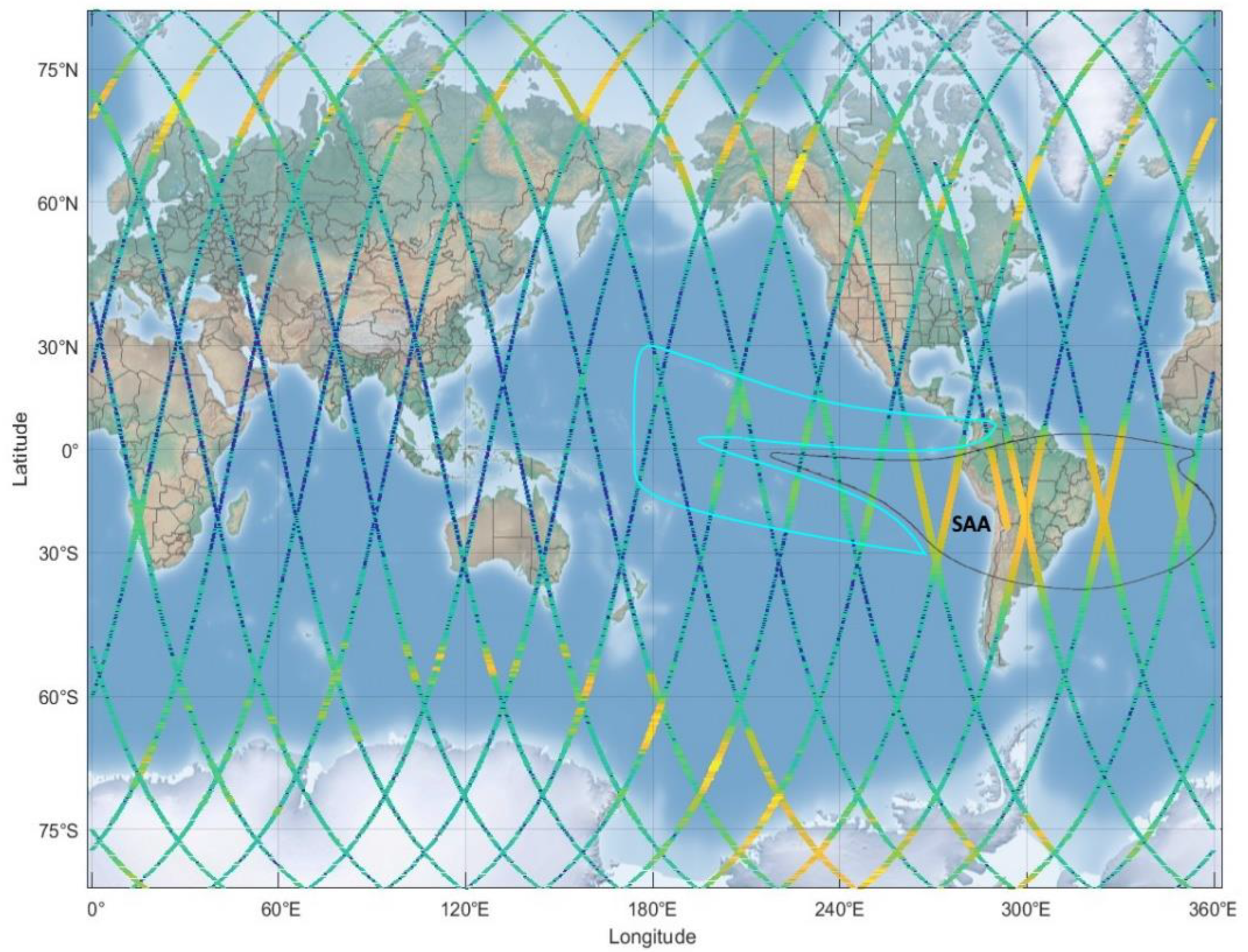
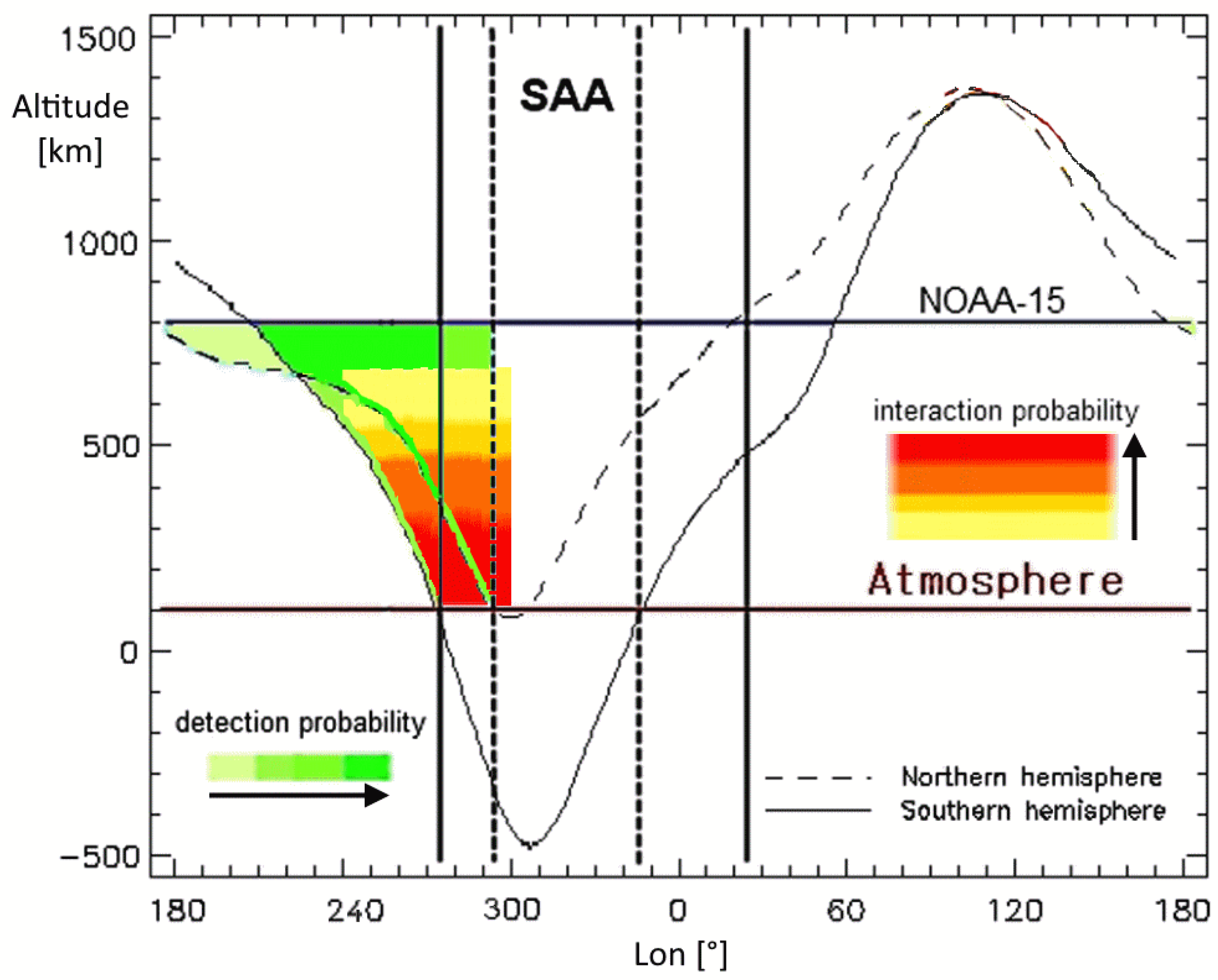
The extraction of EBs from the NOAA-15 database of CRs starting from July 1998 to December 2014 was performed using the same procedure as in previous analyses [26,27,28]. Being so, the starting set of EBs to correlate to EQs remained unvaried and is reported in Figure 2 of a past work [28]. These EBs were all in the loss cone with bouncing altitudes lower than 200 km, and for 95% of cases lower than 100 km, in correspondence to the South Atlantic Anomaly (SAA). 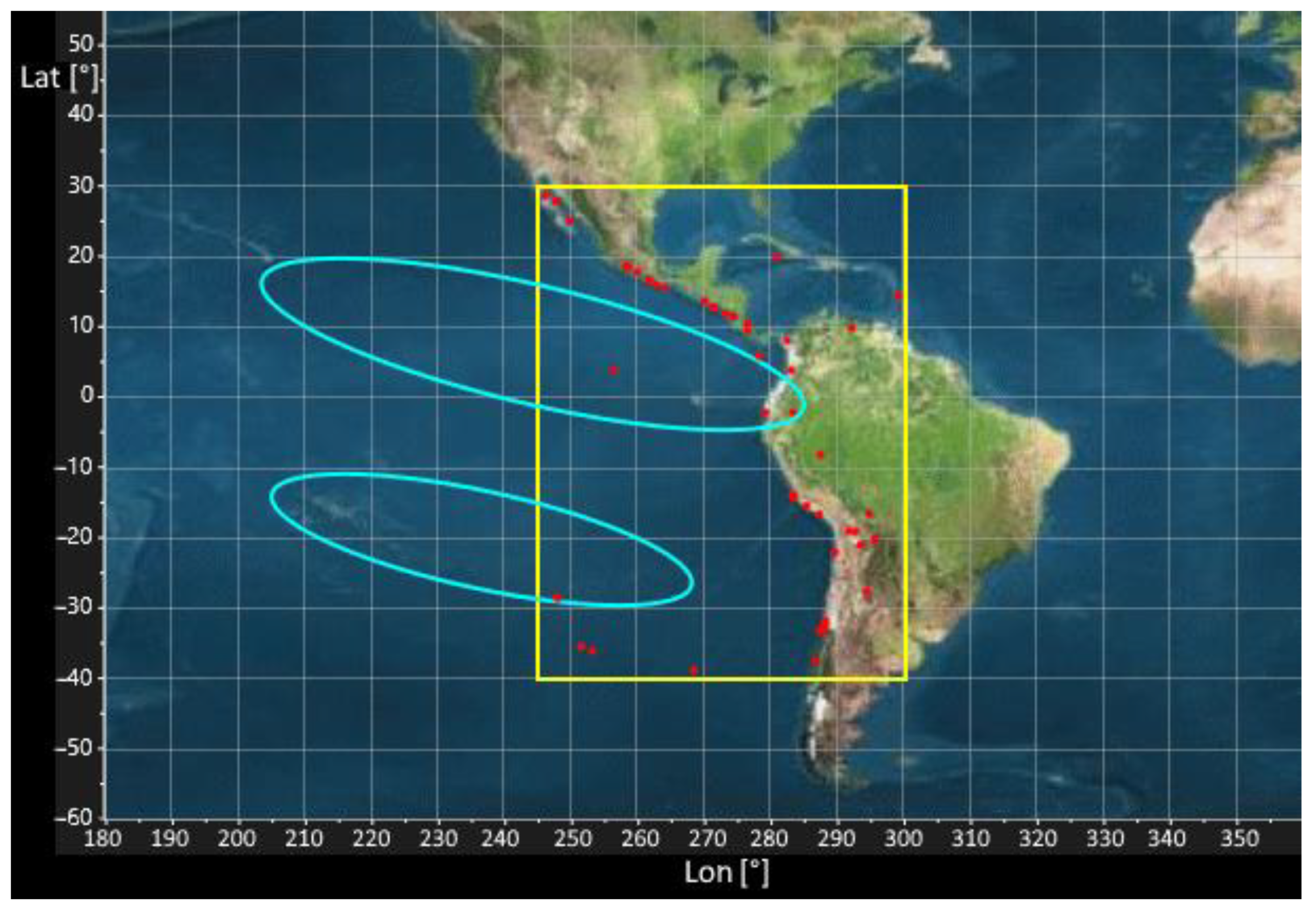Figure 1 reports the geographical distribution of the NOAA-15 trajectories in one day, where the electron flux distribution along the trajectory is represented in colors. The black contour in the center represents the SAA. As reported in previous analysies, see, for example, Figure 1 of [26], precipitating electrons were observed far from the SAA to the west up until 170° in longitude, indicated by the cyan contour of Figure 1. The space-time distribution of the detected EBs consists of a series of consecutive events corresponding to time intervals lasting up to a few minutes. Although, one or more non-consecutive detections characterized the space-time distribution of EBs along the single semi-orbit. Moreover, the observation of one or more EBs in a semi-orbit was defined as only an EB event. Being that the EB L-shells were limited at L < 1.4 by the requirements of precipitating particles from the inner Van Allen Belts, the time length of every EBs was always found less than 12 min. For what concerns the EB time, was defined as the average time among the times of selected EBs in the semi-orbit.

Unlike the previous study [26], which investigated strong EQs worldwide, the subsequent work [28] reported on correlations obtained with EQs restricted to the Philippines and Indonesian areas, in order to maximize the ratio between the correlation amplitude and the non-correlation amplitude. Afterward, numerous geographical areas were tested for their suitability, with the aim of maximizing this ratio, so a stronger correlation was obtained for West Pacific EQs [27]. During our study, the extension of the EQ area was pushed to the Central Pacific until it reached the East Pacific, therein another correlation peak emerged. Given this, a new analysis started for EQs in East Pacific.

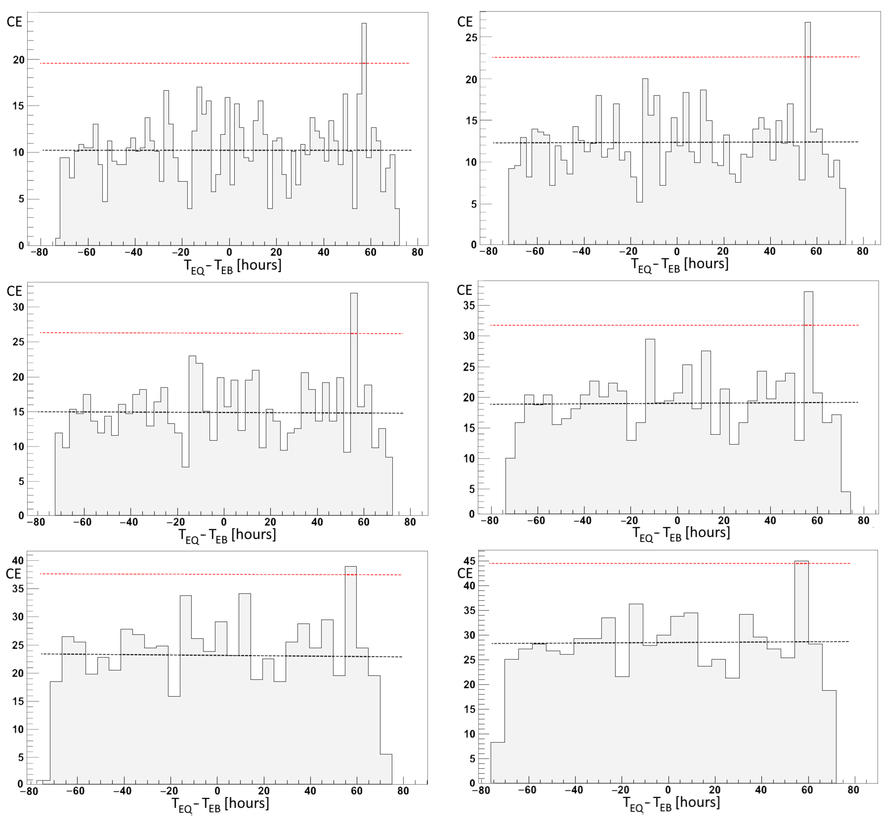
A set of 6 correlation plots between 30–100 eV EBs and East Pacific M ≥ 6 EQs are shown in Figure 2 where the bin time interval was chosen between 2 and 6 h. A range of ±3 days was considered for the time difference between EQs and EBs, where T_EQ − T_EB positive highlights that EBs precede EQs, while EQs precede EBs for negative time differences. CE distributions were Poissonian as in past cases, and the average values are indicated using black dashed lines, while the red dashed lines are used for standard deviations. Significant correlation peaks appear at time differences around 57 h, which means that the EB observation anticipated the corresponding EQ. Unlike past works [26,28], where the correlation significance was represented by EQ projections at certain altitudes, here the correlation significance was calculated exclusively with respect to the EB features. 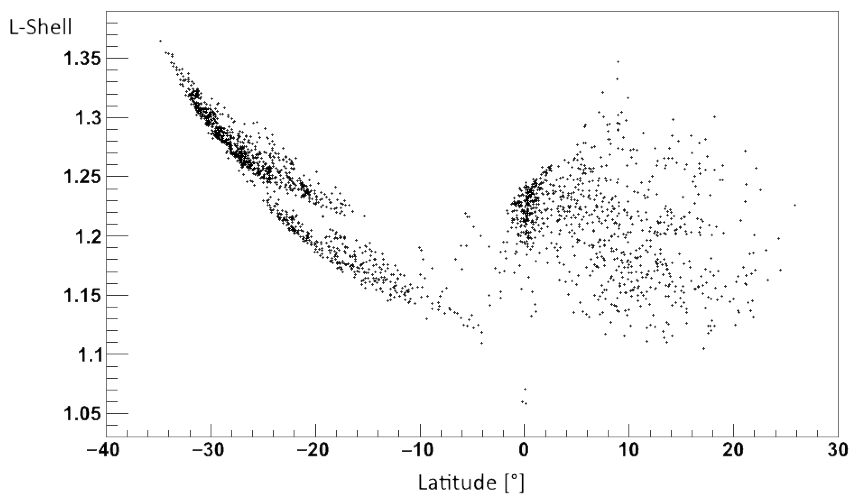In analogy with the case of West Pacific EQs [27], the L-shell interval of electrons to maximize the correlations between EBs and East Pacific EQs was obtained at 1.1 ≤ L ≤ 1.3. A plot of this EB L-shell parameter compared to latitudes is shown in Figure 3. The plot reports two distinct distributions, a correlation for negative latitudes and a lack of correlation for positive ones. For what concerns electron pitch angles, they were concentrated in intervals around 67° and 117°, with 56° ≤ α ≤ 72° and 108° ≤ α ≤ 126°. The correlations in Figure 2 were obtained for EQ depths lower than 200 km, supporting the hypothesis that only EQs close to the surface seem to be correlated to ionospheric activity.

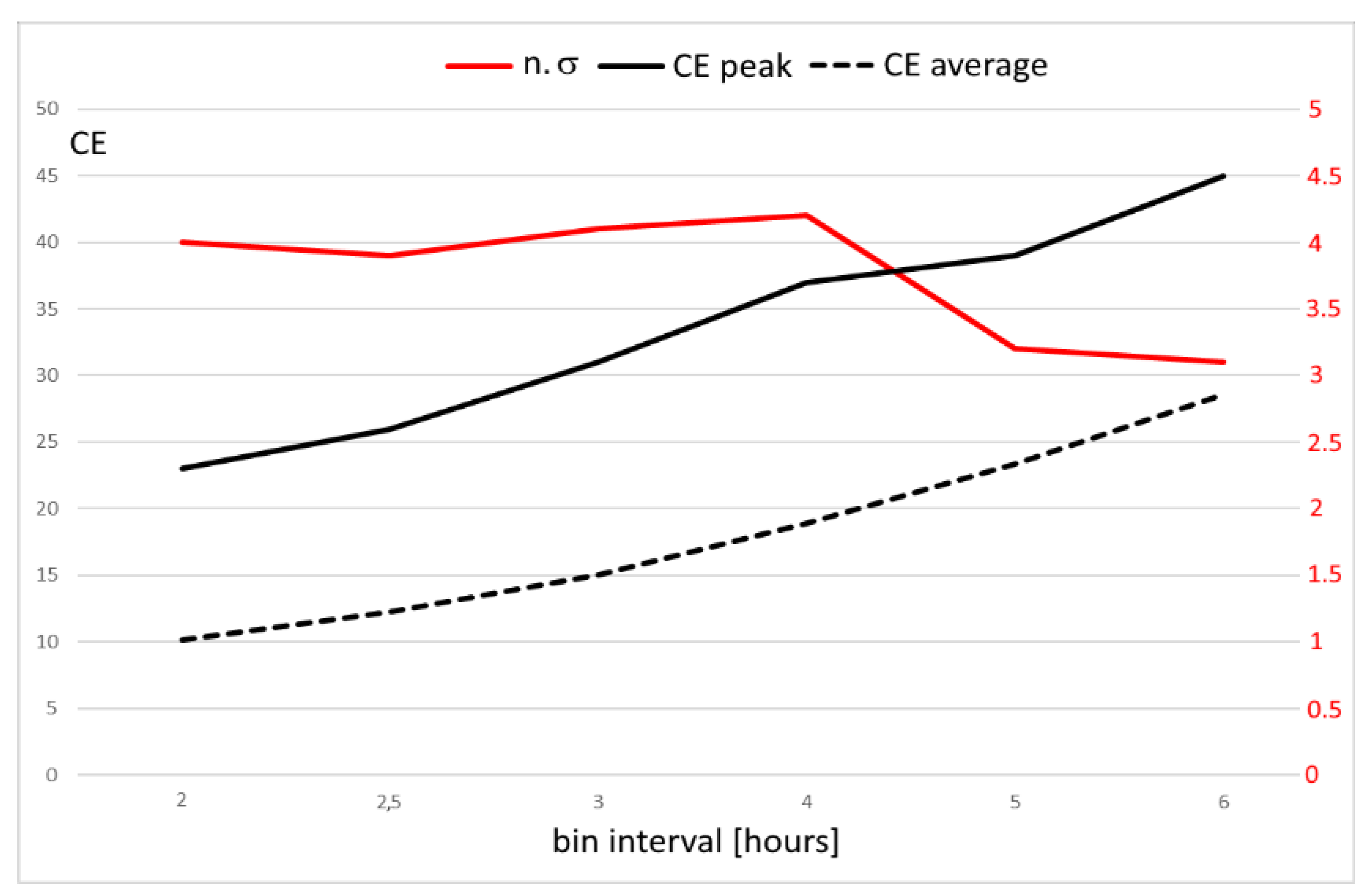
The significance of the correlation peaks was calculated for all the cases shown in Figure 2. The plot shown in Figure 4 summarizes the results regarding the number of standard deviations that define the correlation peak significance above the average values concerning the bin duration and the relative average correlated events. A statistical increase in the correlation peak significances was observed, which started to exceed 3 standard deviations for a bin correlation less than or equal to 6 h and reached a maximum of over 4 for a bin correlation of 4 h. The correlation peak significance was less than 3 for bins greater than 6 h. Concerning the number of correlated events, it decreases for short correlation bins. In Figure 4, a continuous red line indicates the number of standard deviations of 57 h correlation peaks observed with different bins, a continuous black line indicates the number of events at the peaks, whereas the dashed line indicates the averages. All the correlation peak significances overcame the threshold of 99%. As in the past publications, both correlation calculus using a randomized space and time distributions of EQs were also calculated by using the same EQ times, and the same EQ epicenters, respectively. In these randomized cases, the previously obtained correlation peaks completely disappeared.

The maximum number of 45 correlation events was found for the greatest time bin of 6 h, which corresponded to 45 EQs identified in the map in Figure 5. The geographical region where EQs correlated with NOAA-15 EBs is delimited by −40° to 30° in latitude and by 245° to 300° in longitude, the yellow line in Figure 5, so included are regions with strong seismic activity, such as Mexico, Caribbean Sea, Guatemala, Honduras, Nicaragua, Costa Rica, Panama, Columbia, Ecuador, Perú, Bolivia, Chile, and a large part of South-eastern Pacific. EQ epicenters are indicated by red dots in Figure 5, about half of which are located offshore. 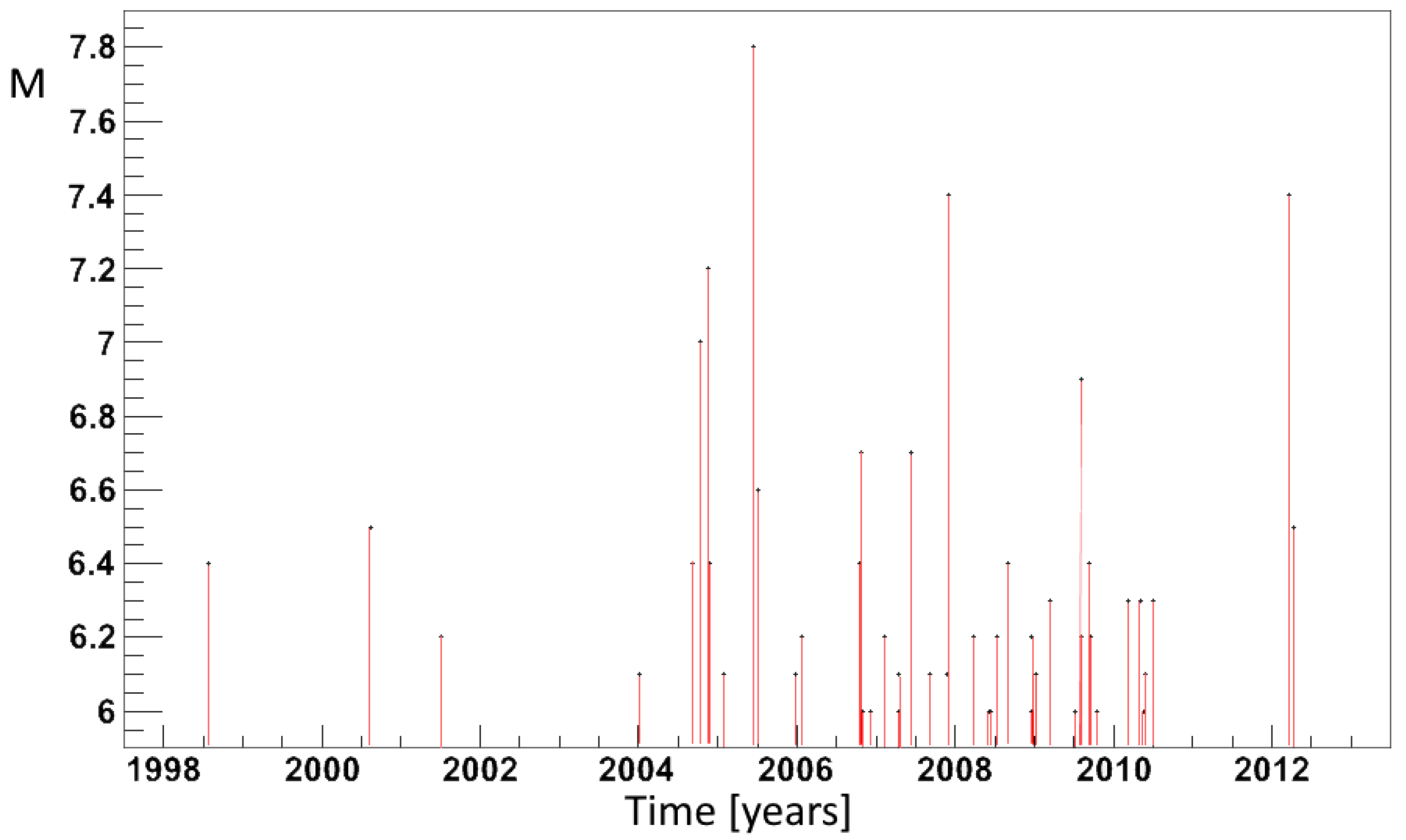Note that the total number of mainshocks that occurred during 16.5 years in Figure 5 yellow square was 199, they were about 1/3 of the mainshocks that stroked West Pacific in the same period. However, the 45 East Pacific mainshocks of the peak correlation are near the 44 EQs of the West Pacific correlation peak, being the East Pacific correlation bin 3 times the West Pacific correlation bin. The time distribution of the 45 considered EQs from July 1998 to December 2014 is shown in Figure 6, with their relative magnitudes. Concerning EB detection positions, the geographical region is delimited at −35° and 20° in latitude, and at 205° and 295° in longitude, divided into two inclined belts indicated by cyan contours in Figure 5 whose inclinations are due to the asymmetry of the geomagnetic field. Finally, electron mirror points of detected EBs over the EQ epicenters are plotted in Figure 7, ranging from minimum altitudes between 100 km and 700 km.

4. Discussion

A comparison of the possible results obtained above for East Pacific EQs with those obtained for West Pacific EQs [27] is useful to describe the similarities and differences between them. The first striking difference was found in the correlation time difference which was a few hours for West Pacific EQs and a few days for East Pacific EQs, even if EBs anticipated EQs. The first striking similarity was found between the maximum CE number. Concerning the CE significance, calculated using the σ number, the results were slightly worse being the maximum significance of a little more than 4, observed for bin intervals of 4 h, compared to a little more than 5 for bin intervals of 2 h of the past. The CE number relative to the maximum significance was lower for the East Pacific case. The geographical positions of EBs were nearly entirely overlapping, with a slight shift to the East of around 10°, whereas the relative positions concerning the correlated EQ epicenters were completely different and non-overlapping. Altitudes of electrons calculated over the new EQ epicenters were also completely different, resulting in many hundreds of kilometers lower compared to past studies. The EQ area in the West Pacific belonged more to the Northern hemisphere than to the area of the East Pacific EQs that belonged more to the Southern hemisphere. This seems to reflect the geomagnetic field asymmetry, following the geomagnetic equator crossing the geographic equator from north to south and moving eastwards to those longitudes. The EQs are instead quite similar for the two regions, being in both cases superficial and equally distributed between land and oceanic crusts.

Concerning the adiabatic parameters of EBs, the L-shell range in this study resulted in being more extended towards lower values, and the latitude dependence was lost for positive latitudes. Moreover, the positive latitude dependence of L-shell was observed for EBs over West Pacific EQ epicenters around 125°, see Figure 2 of [27]. However, EB longitudes over East Pacific EQs are close to the SAA, where the geomagnetic field deviates from the dipolar shape. Specifically, the angle between the satellite’s orbit and the geomagnetic line is small for positive latitudes and close to 90° for negative latitudes. Therefore, the satellite crosses the 1.1 ≤ L ≤ 1.3 in more than 20° of positive latitude, whereas it crossed the same interval in 5° of negative latitudes. In fact, the pitch angle of positive latitude EBs is restricted to 56° ≤ α ≤ 72° while the pitch angle of negative latitude EBs is restricted to 108° ≤ α ≤ 126°. Furthermore, two different distribution bands were observed, see Figure 3, for negative latitudes. They were separated approximately by α = 120°, with 1.1 ≤ L ≤ 1.22 in the interval 108° ≤ α ≤ 120° and with 1.22 ≤ L ≤ 1.3 in the interval 120° ≤ α ≤ 126°. The pitch angle results are divided into two intervals for both studies, coinciding exactly. Being so, the striking difference in the correlation times between the two studies seems to be more naturally associated with the major difference retrieved from the correspondent analyzed data of the two cases: which is the altitude of electrons passing above the East and West Pacific EQs. If the Lithosphere-Ionosphere interaction occurs above the future epicenters and the magnitude depends on the distance of electrons from the lithosphere; as previously proposed for magnetic pulses [6], a lower altitude of charged particles above the East Pacific means that lower magnitude magnetic pulses could be able to modify electron trajectories, even if the general behavior of magnetic pulses have not been proven decreased with the temporal remoteness of strong EQs. Case studies based upon data from the DEMETER satellite of East Pacific EQs, such as the Chile EQ M = 8.8 on 27 February 2010, and the Haiti EQ M = 7.0 on 12 January 2010, recorded similar delays with electron detections [34], also associated with VLF wave activity.

Preparedness for strong EQs and tsunamis has been developed over recent decades [35] either by triggering early warnings or by rapidly assessing the expected damages [36]. Early warnings consist of alerts seconds before the arrival of destructive seismic waves in populated regions. Such an alert may be useful in controlling the shutdown of gas pipelines and critical facilities, reducing speeds of rapid-transit vehicles, and also advising the interested populations to follow the necessary precautions. Reduced lead times limit the possible preparedness actions, thus leaving part of the population at the mercy of imminent danger. Utilizing the possible correlation results obtained above for a short-time warning in strong EQs and tsunami preparedness might contribute to reducing the impact of EQs.

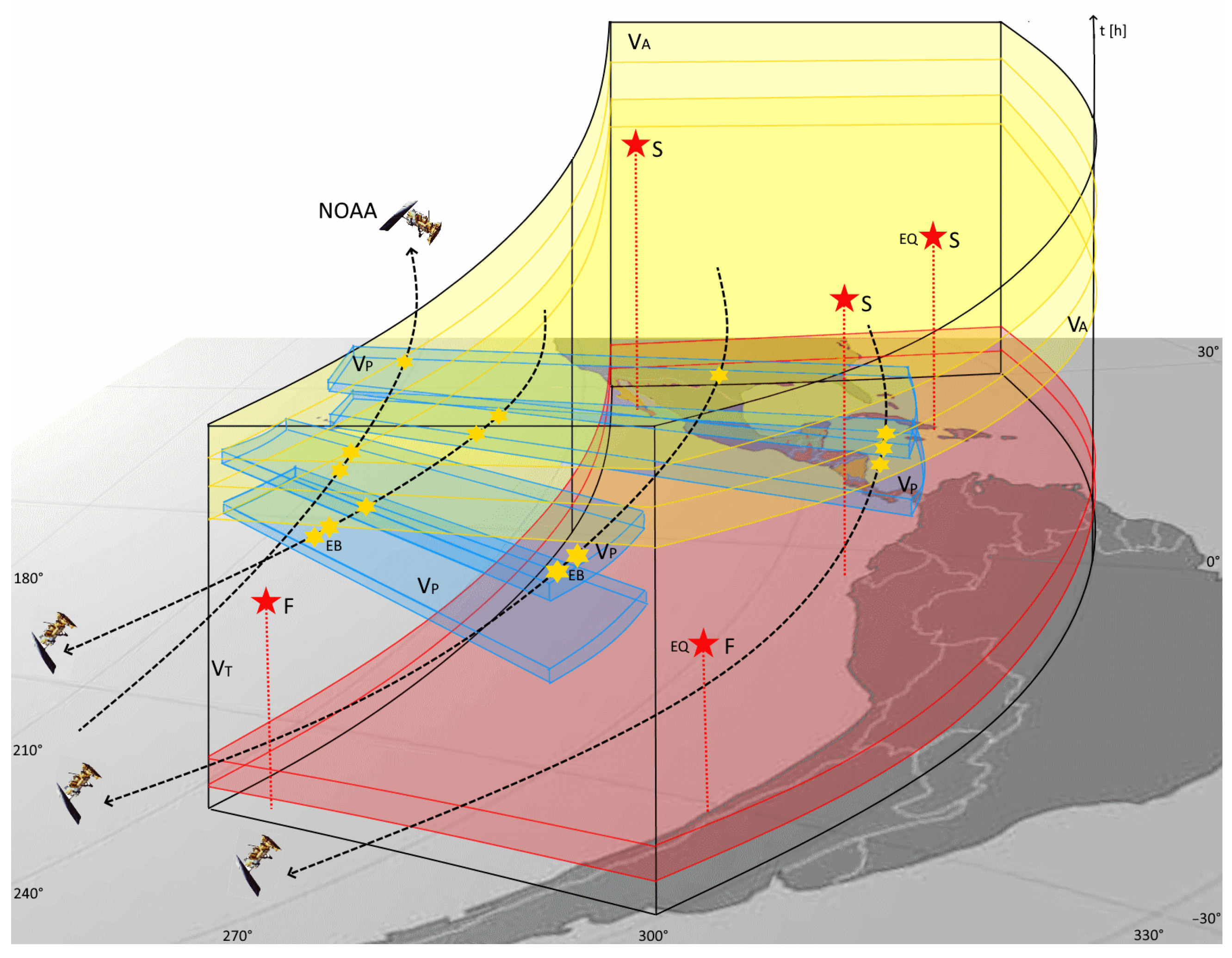
A way of using such results is to define a scenario for a short-time prediction model [27]. Following the work of Console [37], the representation of the EQ prediction model would need to define the target volume where EQs occur V_T, which is a 2-d geographic space + 1-d time-space. This volume is displayed by a black contour in Figure 8, and with EQs occurrence by red stars. If an EQ occurs in the alarm volume V_A in yellow, it is a success (S), while if an EQ occurs out of the yellow volume it is a failure of prediction (F). The precursor volume V_P, which is generally different from V_T, contains the alarm events. In this case, V_P is the cyan volume of Figure 8 where EBs are detected, the time of EB observations lasting less than 12 min. When an EB is detected in V_P it is an alarm that defines a V_A. The time span of the EQ observations multiplied by the area of East Pacific where the correlations in Figure 2 are calculated is V_T. An EQ event is included in this scenario only if M ≥ 6. Unlike West Pacific earthquakes where geographical areas of V_P and V_A were completely disjoined, areas of EQs and EBs are largely overlapping in this scenario. In this representation, V_A has the dimension T which coincides with the correlation bin dimension, it is generated by an EB detection in V_P, and covers the same area as V_T. To have the greatest significance the 4 h bin interval of 54.3–58.3 h should be chosen. The V_A dimension and shape are the same for each detected EBs in V_P; if an EQ with M ≥ 6 occurs in V_A one success is collected. Similarly, if an EQ occurs out of the V_A, meaning that it happened before or after the 4 h between the 56.3 h following the EB, one failure is collected. Moreover, one false alarm is collected for any EB detection not followed by any EQ. Non-continuous V_T is defined as when the Sun’s activity leads to discarding days or due to the NOAA-15 satellite intermittence into the detection area west of the SAA. A V_A is generated within V_T 56.3 h after an EB is detected in V_P, and the time ahead is the vertical distance in the representation of Figure 8.

The V_T can be obtained by multiplying the East Pacific area by the total number of hours [27], this total number corresponds to N_h = 36,135 for 4 h intervals. The following was observed in V_T: a total number of N_EQ = 199 EQs with M ≥ 6 and depths ≤ 200 km, resulting in a P(EQ) = 0.0055, a total number of N_EB = 3371 EBs which are alarms, and a total number of N_S = 37 CEs which are successes. 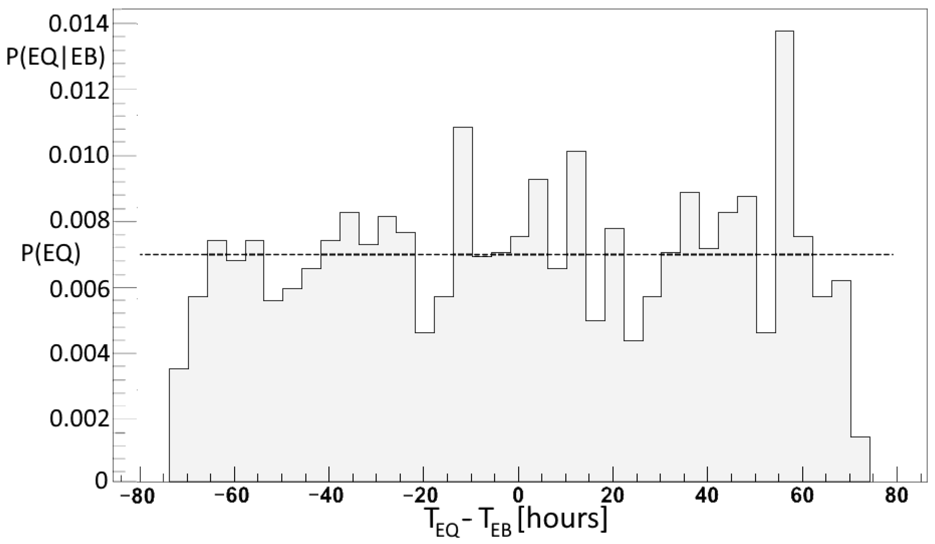The success rate was calculated by N_S/N_EB = 0.011, which is the conditional probability (1) [27], 1 − (N_S/N_EB) = 0.989 is the false alarm rate, while the alarm rate is N_S/N_EQ = 0.186, and the failure rate is 1 − (N_S/N_EQ) = 0.814. As there were more alarms than those for the West Pacific EQs, with the success being near the same for the two cases, the number of false alarms in this study increased compared to previous research. A cross-correlation of 0.024 was calculated using the relation (3). The EQ occurrence probability of at least one target event was estimated to be P(EQ) when no EB was observed two and a half days before, while it increased to P(EQ|EB) given by (2) two and a half days after the EB observation. The probability distribution is shown in Figure 9, which indicates a probability gain near G = 2. As for the study in the West Pacific [27], days with more than one burst can be found with a frequency of about 20%, and EBs belonging to successive orbits generated a partial overlapping between two consecutive alarms. These are not considered here and will be presented in a future publication.

An early warning system for evacuation should be based on effective EQ observations [37]. However, the geohazard risk reduction can gain valuable preparation time by adopting a probabilistic short-term warning a few hours prior, especially for tsunamis [36]. Thus, using NOAA-15 electron CR analysis is in principle achievable based on the infrastructure of antennas operating along the West Coast of the US [28], at the same longitude where EBs are detected. The system would need to be able to download NOAA data early enough so it can be analyzed in a few minutes and then compared with geomagnetic activity within a day. 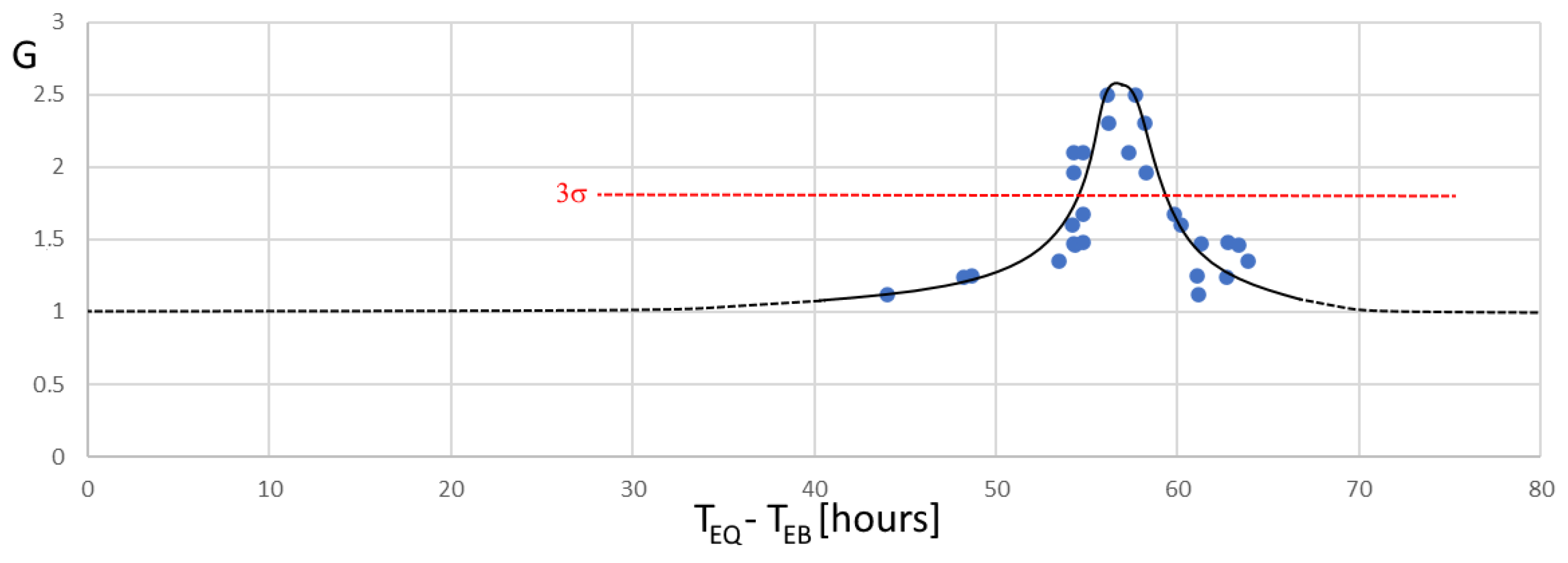As EBs were detected in the same region where they anticipated West Pacific EQs [27], the probability of a strong EQ in the West Pacific cannot be neglected, which would vanish in less than 4 h. Then, if no strong EQs occur in the West Pacific, based on completely statistical evaluations of disastrous events presented in this work, an East Pacific coast forecasting can be generated using G increases in EQ-probability. Moreover, correlation bins of time lengths greater than 6 h were investigated, they concerned the cases of 7, 8, 9,10, 12, 14, and 17 h. A decrease in significance was generally observed for the corresponding correlations, where the sigma decreased up to 1.1 for the 17 h case. Furthermore, the probability gain was calculated for each bin and reported in the plot of Figure 10 for each starting/ending time of the correlation peak. The case of 1.5 h was also added to this plot. A fit of the G distribution is reported in Figure 10, which can be interpreted as the time-dependent conditional probability of a strong EQ in the East Pacific area after an EB has been observed at time 0. Figure 10 shows that an increase in conditional probability is observed at about 40 h from the NOAA detection, around 54 h the probability magnitude overcomes the 99% significance level up to around 59 h. Finally, the probability decreases at an unconditional level around 70 h after the EB detection.

5. Conclusions

A new statistical correlation analysis between precipitating EBs and strong EQs was carried out from the analysis of exactly 16.5 years of NOAA-15 particle data. This seemed to indicate that electrons in the loss cone were mainly observed around 57 h before main shocks with M ≥ 6 in the East Pacific, comprising countries where seismic activity is frequently a danger. Results are in line with previous single-case observations by the DEMETER satellite. The new correlation time is significantly longer than the correlation time found for strong West Pacific EQs, with EBs occurring a few hours prior. It again supports the hypothesis that there might exist a link between ionospheric and lithospheric activities of shallow EQs whose depths are less than 200 km. As for West Pacific EQs, also this correlation happens regardless of whether the EQs occurred in the sea or on the mainland.

The parameter L-shell of the electrons was defined uniquely, as in the previous publication on West Pacific EQs [27], therein providing a precise definition of an EB to also carry out an EQ forecast in the East Pacific. The L-shell distribution in this new case was distributed differently in terms of latitude, compared to the West Pacific case, which probably reflects the asymmetry of the geomagnetic field. A probability gain G = 2 was calculated which could be used to increase the pre-alarm time of some early warnings for both strong EQs and tsunamis on the East Pacific’s coasts. Despite the high number of false alarms being greater than in the West Pacific case, a time-dependent conditional probability interpretation of the process was proposed.