Abstract
Unmanned aerial vehicle (UAV) inspection has become the mainstream of transmission line inspection, and the detection of insulator defects is an important part of UAV inspection. On the premise of ensuring high accuracy and detection speed, an improved YOLOv5 model is proposed for defect detection of insulators. The algorithm uses the weights trained on conventional large-scale datasets to improve accuracy through the transfer learning method of feature mapping. The algorithm employs the Focal loss function and proposes a dynamic weight assignment method. Compared with the traditional empirical value method, it is more in line with the distribution law of samples in the data set, improves the accuracy of difficult-to-classify samples, and saves a lot of time. The experimental results show that the average accuracy of the insulator and its defect is 98.3%, 5.7% higher than the original model, while the accuracy and recall rate of insulator defects are improved by 5.7% and 7.9%, respectively. The algorithm improves the accuracy and recall of the model and enables faster detection of insulator defects.
1. Introduction
During the routine inspection of transmission lines, the main methods include manual inspection, helicopter inspection, robot inspection, and unmanned aerial vehicle (UAV) inspection [1]. With the development of technology, UAVs have gradually become an important method for transmission line detection because of their low cost, convenient operation, and high efficiency. Power supply companies take a large number of inspection pictures during daily inspections through drone inspections. However, these pictures currently mainly rely on manual recognition, which is less efficient and accurate. Therefore, using deep learning technology to detect insulator defects quickly and accurately is the new direction of power inspection development [2].
In recent years, with the development of deep learning theory and the improvement of computer hardware performance, the research on transmission line defect detection based on deep learning has become a hot topic. At present, there are two main kinds of neural networks commonly used in target detection. The first is a two-stage target detection model based on region extraction, such as faster region-based convolutional neural networks (Faster R-CNN) [3], and the second type is based on regression single-stage target detection, such as “You Only Look Once” (YOLO) [4], Single Shot MultiBox Detector (SSD) [5], etc. These two models are widely used in current research. For example, Manninen et al. [6] proposed a new method for assessing the condition of transmission overhead lines, which can automatically isolate transmission poles, disaggregates components, detects defects, and determines the health index of concrete structures and insulators, compared to traditional foot patrol visual inspections. This approach greatly improves efficiency and reduces costs. Hosseini et al. [7] have developed a model for automatically estimating and locating the damage process of distribution rods, which uses images taken by drones to be transmitted in real time to the Intelligent Damage Classification and Estimation (IDCE) unit. The model has high accuracy in the classification and estimation of the damage of distribution poles. Liang et al. [8] proposed a method of fault detection and evaluation of transmission lines based on deep learning is presented. It can effectively identify eight transmission line component defects, such as insulator defects, three-plate defects, damper defects, graded ring defects, etc., as well as nesting and foreign objects attached to the transmission line. Wanguo et al. [9] proposed an SSD algorithm based on candidate regions to locate and identify insulator and anti-vibration hammer defects. Zhao et al. [10] constructed an automatic defect detection model called Automatic Visual Shape Clustering Network (AVSCNet) for the detection of missing parts of bolts, and its detection accuracy can reach up to 87.6%. Qiu et al. [11] proposed a method for detecting insulator defects based on an improved YOLOv4 algorithm. Graph Cut-based image enhancement and Laplace sharpness were used to preprocess insulator images, and YOLOv4 model architecture was improved using Mobile Net lightweight convolution neural network. Combined with the migration learning method, the detection accuracy can be improved to 97.26% after image preprocessing. Zhang et al. [12] proposed an optical image detection method based on deep learning and morphological detection. Faster RCNN is used to locate insulators and extract their target image from the detection image. A mathematical model is built to describe the defect in the binary image to improve the precise location of the defect.
The detection effect of the method based on deep learning is greatly limited by the amount and distribution of data. Unbalanced data samples will have a greater impact on the detection results. The number of intact insulators in transmission line defect detection is much larger than the number of insulators with self-burst defects. This results in the model not being trained effectively, making it difficult to improve the performance of defect detection. Many researchers have studied the problem of data sample distribution and difficult-easy imbalance. Shrivastava et al. [13] propose an online method for mining Online Hard Example Mining (OHEM) for difficult samples. This method can optimize the model to improve the detection performance by using the variation of sample loss size during training to select difficult samples. Li et al. [14] proposed a Stratified Online Hard Example Mining (S-OHEM) algorithm for training more efficient and accurate detectors. S-OHEM utilizes the OHEM of stratified sampling (a widely adopted sampling technique) to select training samples based on this influence during hard sample mining, thereby improving the performance of object detectors. Lin et al. [15] proposed to address the sample imbalance problem by reshaping the standard cross-entropy loss, thereby reducing the weight of the loss assigned to well-classified examples. They designed a Focal loss function that adjusts its contribution to the loss function according to the confidence of the detection results, thus solving the problem of imbalance between positive and negative samples and hard samples in phase detectors. Li et al. [16] proposed to use the gradient density distribution to explain the influence of the unbalanced distribution of positive and negative samples and difficult and easy samples on the results, and further proposed a gradient harmonizing mechanism (GHM) to overcome its negative effects. This mechanism can improve the effects of loss functions such as CE and Smooth-L1 in anchor classification and box regression problems, respectively. Li et al. [17] proposed a YOLO-ResNet model for rebar detection. The YOLO-ResNet model adds the convoluted block attention module (CBAM) attention model to the input and output sections, introducing a Focal loss function to punish easily divisible negative samples and allowing the model to converge faster. The results show that the YOLO-ResNet model has better performance, less training time, lower GPU memory usage, and smaller model weight files, and does not reduce the detection accuracy in steel bar detection. Li et al. [18] proposed a deep learning-based automatic detection framework for nests, called Area of Interest (ROI) mining for faster area-based convolution neural networks (RCNN). By using k-means clustering, the Focal loss function is introduced, and the ROI mining module is added to solve the class imbalance in classification stage. Experiments show that the high accuracy of bird’s nest detection can be achieved. Li et al. [19] have designed an improved cross-entropy loss function that pays more attention to difficult samples and uses it for faster R-CNN. The experimental results show that the precision of the difficult sample can be improved effectively, and the total precision can be improved. Dai et al. [20] chose the fast and efficient lightweight YOLO v5 as the base network. The robustness of the model was improved by repetitive broadening, focusing, and smoothing of BCE strategies, and the imbalance of positive–negative sample ratio was resolved. Images of 59 crop disease types across 10 crops showed an average identification accuracy of 94.24%, an average reasoning time of 1.563 milliseconds per sample, and a model size of just 2 MB. Compared with the original model, the model size was reduced by 88% and the inference time was reduced by 72%. Cao et al. [21] proposed a high performance algorithm, which realizes real-time detection and traffic statistics by adjusting network structure, optimizing loss function, and introducing weight regularization. The experimental results show that the YOLO-UA model has high accuracy, precision and recall rate for different weather scenarios, and has good robustness with low impact on scenario and weather variation. Liu et al. [22] proposed a Cross Stage Partial Dense YOLO (CSPD-YOLO) model based on YOLO-v3 and the Cross Stage Partial Network. The CSPD-YOLO model uses the characteristic pyramid network and improved loss function to improve the accuracy of insulation fault detection. The average accuracy of the CSPD-YOLO model was 4.9% and 1.8% higher than that of YOLO-v3 and YOLO-v4, respectively.
To sum up, in the existing methods and literature, the Focal loss function is introduced to solve the uneven distribution of positive and negative samples and difficult and easy samples. However, for the two weight factors in the Focal loss function, most of them adopt the method of empirical value. There are several problems in the results of training according to the empirical method. First of all, the existing methods determine the weights based on experience, and it is difficult to adjust dynamically according to the distribution ratio of positive and negative samples, and difficult and easy samples. Secondly, the accuracy of the model trained by the recommended empirical values may not be the optimal solution. Finally, training after multiple adjustments to the two weighting factors takes a lot of time and computational resources.
In order to solve the above problems, this paper uses the YOLOv5 as the basic model, introduces the pre-trained weights trained on large-scale data sets for transfer learning, and uses the Focal loss function to replace the cross-entropy loss function. The two weighting factors in the Focal loss function are redesigned so that they can change dynamically based on the dataset. Finally, the training result of the original model is compared with the training result of the improved model. The improved detection model was also compared experimentally with Faster R-CNN, SSD, YOLOv3, and YOLOv4. The results show that the method proposed in this paper has high accuracy and short training time and can be used as a reference for the defect detection of transmission line insulators.
2. Materials and Methods
2.1. Introduction to Algorithm and Network Structure
The YOLOv5 [23] model was presented in 2020 and is at a relatively high level of speed and accuracy of detection. The model can choose different network depths and feature diagram widths according to the requirement of accuracy and speed. The official code of YOLOv5 provides five versions: YOLOv5n, YOLOv5s, YOLOv5m, YOLOv5l, and YOLOv5x. In this study, due to the small number of insulator datasets and the high requirement for recognition speed, YOLOv5s is selected as the basic training model in this paper. Figure 1 shows the specific structure of the YOLOv5 network model.
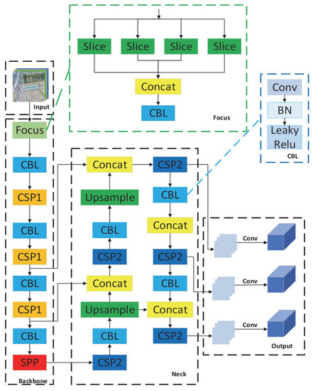
Figure 1.
YOLOv5 network model structure diagram.
The YOLOv5 network is mainly divided into four parts, namely input, backbone network, neck network, and output. At first, the adaptive anchor frame is calculated by K-means clustering to improve the accuracy of locating small target defect of broken insulator. Backbone is mainly used to extract image features, mainly using Focus and Cross Stage Partial (CSP) Network structures compared to previous generations. The Focus structure slices through the incoming images, reducing the computation. The CSP structure [24] is used to accelerate reasoning and speed up training while ensuring accuracy. FPN [25] and PANet [26] multi-scale feature fusion are used in the Feature Fusion Module to output detection results at different feature levels, not only improve the detection rate and the localization and recognition accuracy of each scale target, but also combine CSP structure fusion features to optimize feature fusion speed. Finally, the target box is regressed by CIOU loss function [27], and the binary cross-entropy loss function is used for classification and confidence regression. The detection output section eliminates redundant target boxes by non-maximum suppression (NMS) [28], predicts image features, generates boundary boxes, and predicts categories.
The loss function of YOLOV5 consists of three parts: classified loss, rectangular loss, and confidence loss, which are weighted together to form the ultimate loss function. As shown in Equation (1).
Among them a, b, c is the weight of each of the three loss functions, usually, confidence loss gets the maximum weight, rectangular loss and classified loss are the next most weight.
The classification loss and confidence loss functions used by YOLOv5 are two-class cross-entropy loss, and the formula is shown in Equation (2). Where N is the total number of categories, is the true value of the current category and is the predicted probability of the current category.
Classified loss function is mainly used to predict the category of each lattice in three classification boxes. The confidence loss function is mainly used to predict the confidence of each prediction box, that is, the reliability of the prediction box. The greater the confidence value, the more reliable the prediction box is, that is, the closer to the true minimum box of the target.
Binary cross-entropy is used to judge the difference between the predicted result of a classification model and the true value. If the predicted value is closer to 1, then the value of the loss function should be closer to 0, that is, the smaller the difference between the predicted result and the true value, the smaller the value of the loss function. Conversely, if the predicted is closer to 0 at this point, that is, the greater the difference between the predicted result and the true value, the greater the value of the loss function.
2.2. Improved YOLOV5 Model
To detect defect locations of insulators more efficiently, pretrained weights are introduced in YOLOv5. Second, the Focal loss function is introduced to reduce the defect detection rate due to the imbalance of positive and negative samples, the difficulty of insulator and defect classification, and the Focal loss function is optimized by dynamically calculating the weight factor.
2.2.1. Pretrained Weight Transfer
At present, the target detection algorithm based on deep learning technology needs sufficient training samples to train the model on a large scale in order to achieve relatively good detection effects. In this paper, the insulator and its defect dataset are small, especially the defect sample data are smaller, so it is easy for the model to be overfitted and the accuracy and recall rate is low. Individuals have fewer computing resources and cannot conduct large-scale dataset training. Therefore, this paper uses transfer learning to learn prior knowledge from COCO128, a large-scale data set trained by companies with large computing resources. Migrating the corresponding weight parameters from COCO128 to the data set of this paper can accelerate the convergence speed of the loss function of the model, and the accuracy rate and other indicators can be quickly improved to a higher level. The main methods and applications of migration learning are shown in Table 1. Because the source dataset contains a large number of different categories and is different from the insulator defect dataset in the paper, the paper adopts a migration learning method based on feature mapping.

Table 1.
Scenarios for migration learning methods.
2.2.2. Focal Loss
Focal loss is a loss function based on binary cross-entropy [29]. It is a dynamic scaling cross-entropy loss function that can reduce the weight of easily distinguishable samples in training. The method can help net quickly focus on difficult samples, both positive and negative, that are helpful to the training network. Its formula is shown in Equation (3).
where is the Focal loss function, the α weight factor is used to regulate the balance between positive and negative samples, the γ weight factor is to regulate the weight balance between difficult samples. is the true value of the tag, 1 is a positive sample and the rest is a negative sample, is the predicted value output by the network model. The attenuation curve of the Focal loss function is shown in Figure 2. The smaller the difference between the predicted and true values, the smaller the loss value, indicating that the sample at this point is an easily classified sample. The greater the difference between the predicted and true values, the greater the loss value, indicating that it is more difficult for the sample to be correctly predicted at this time. When γ is 0, the loss function is the cross-entropy loss function, and the value of the loss function changes more smoothly than the predicted value. At this point, if there are a large number of easy to categorize samples, the loss of their contribution will dominate the whole loss function, making it difficult to optimize the model. When the value of γ increases gradually, the difference between the predicted value and the real value is smaller, the sample is classified easily, and the contribution of loss value is small. When the difference between the prediction and the real value is greater, the sample is difficult to classify, and the contribution of loss is large. In this way, in the process of model optimization, the loss value of the difficult sample will dominate the optimization of the model more and improve the accuracy of the difficult sample.
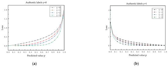
Figure 2.
Focal loss decay curve. (a) Authentic labels y = 0. (b) Authentic labels y = 1.
2.3. Dynamic Weight Calculation
In the Focal loss function, since there is no standard value protocol for the weight factors α and γ, the values need to be selected according to the sample distribution of the dataset. The empirical values of 0.25 for α and 2 for γ were commonly used in the results presented in the literature [15]. However, empirical methods do not necessarily apply to all datasets and need to be dynamically adjusted according to the dataset itself and the variation in the distribution of positive and negative samples and difficult samples during training. By adjusting the alpha and gamma values, we can obtain a better detection network, but the disadvantage is that the alpha and gamma values require us to continuously adjust the training process, which inevitably interrupts the network training process, thus prolonging the network training time. Therefore, in the paper, the two hyperparameters α and γ are designed as parameters that can be dynamically adjusted during the network training process. α is defined as Equation (4).
where is the number of positive samples in each feature map. is the number of negative samples in each feature map.
At the output end of the YOLOv5 network, three feature diagrams of different sizes are generated after each iteration and then matched with a predesigned nine prior bounding box. The feature map is the feature of different scales extracted from the image after the image input to the network is convolutional. These three feature maps of different scales are used to predict the target in the image and generate the corresponding information of the target frame.
Every three prior bounding boxes are matched with one feature map, and when the aspect ratio of the prior bounding box to the real box was lower than the threshold it was a positive sample and higher than the threshold it was a negative sample. Therefore, the number of positive and negative samples on three different feature diagrams is not the same. By calculating the number of positive and negative samples on each feature map, the proportion of positive samples in the overall sample can be calculated. In the algorithm, the ratio of positive samples to population samples on each feature map is first calculated. Second, the scales obtained on the three feature maps are summed. Finally, the result of the addition is averaged as the value of α. The ratio of positive to negative samples varies according to the characteristic diagrams generated during each iteration, and α varies according to the ratio of positive to negative samples. Positive and negative samples can be given different weights by changing α. Positive samples are given a larger weight, and negative samples are given a smaller weight.
Additionally, γ is defined as Equation (5).
where is the true value of each predicted object, 0 or 1. is the prediction confidence. γ is mainly used for the adjustment of difficult and easy samples. The division of difficult and easy samples mainly depends on the difference between the predicted value and the actual value. In addition, the difference between the predicted value and the true value is between 0 and 1. Therefore, the design of γ in this paper is obtained by amplifying the difference between the predicted value and the actual value by the formula of the exponent . Through the exponential formula of , the value range of γ can be limited between 1 and 2.7. Compared with the fixed 2.0 value, it has a more flexible value space. During each iteration, the network makes probabilistic predictions for each prediction box, calculating γ by the difference between each prediction and the true value. When the predicted value is different from the real value, the result shows that the sample is difficult to classify and the calculated γ is larger, so the contribution of the difficult sample to the loss function can be improved. When the difference between the predicted value and the true value is small, the sample is classified easily and the calculated γ is small, thus reducing the contribution of the easy sample to the loss function.
The dynamic Focal loss function proposed in this paper omits the manual setting process of hyperparameters. There is no need to have a deep understanding of the distribution of the dataset for training, or knowledge about the convergence of neural network training. This dynamic change method can be adjusted automatically according to the distribution calculation of the sample itself during each training, which can highlight the learning focus of different stages and converge in the direction of global optimization.
3. Experiment and Dataset
The transmission line insulator defect detection model is aimed at problems such as too small insulator defect size in transmission line inspection images, some insulators that are not significant in the real environment, serious overlapping and occlusion of insulators, and slow model detection. This paper proposes an improved YOLOv5 algorithm model to achieve fast and accurate detection of insulator defects during transmission line inspection. The insulator defect detection process is shown in Figure 3.
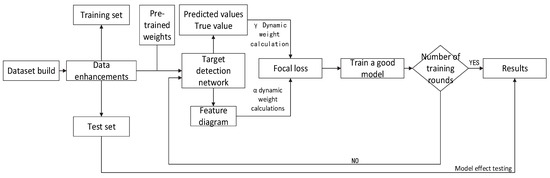
Figure 3.
Detection process of insulators on transmission line.
3.1. Dataset Construction
The data on insulators and their defects in the experiment came from the China Power Line Insulator Dataset (CPLD), which contains 848 aerial and synthetic defect images taken by drones. Another part came from 333 images of defects in glass insulators collected by National Grid Power’s inspection data. The number of two combined for 1181. Insulator defects usually include damage, fragmentation, missing, and other conditions. Due to the limitation of the insulator defect dataset, the paper mainly focuses on the missing insulator sheets, which is the most common insulator defect. A large amount of data is required in target detection missions, so the 1181 insulator images in the dataset are expanded to 2280 images by stochastic brightness, random shear, and random translation, and the positive angles are rotated by 10°, some of which are shown in Figure 4. For the constructed insulator defect dataset, 80% of the images in the dataset are selected as the training set, and 20% of the images are selected as the test set. Due to the different resolutions of different images in the constructed insulator dataset, in order to adapt to the resolution requirements under the YOLO framework, all images are rescaled to 640 × 640 resolution. The number of labels and label boxes of the dataset are shown in Figure 5.

Figure 4.
Data-enhanced renderings. (a) Original. (b) Random brightness. (c) Rotated. (d) Random translate.
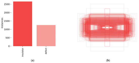
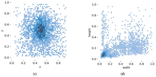
Figure 5.
Data set analysis. (a) Number of insulators and defect labels. (b) Label visualization. (c) The center point of the label distribution. (d) Distribution of label aspect ratios.
Use the image tagging tool called Labelme to tag all images. Insulators are labeled insulator, defect location is labeled defect, and the number of each labeling category is shown in Table 2. The production of the dataset was completed by the above-mentioned work.
Table 2.
Dataset label distribution table.
3.2. Deep Learning Environment Configuration
The hardware environment configuration of this experiment is shown in Table 3. The software environment is: Windows11, Pytorch1.1, Python3.7, CUDA11.2. The batchsize of the model is 32, the initial learning rate is 0.01, the weight decay coefficient is 0.0005, and the total number of epochs is 100.
Table 3.
Experimental environment configuration.
3.3. Evaluation Metrics
The experimental results were evaluated using precision (P), recall (R), and mean average precision (mAP). Accuracy rates were used to measure the classification effect between different categories of the overall model, recall rates were used to measure the overall effect of the model across different categories, and mean accuracy was used to measure the overall accuracy of the model. The formula is as follows:
Among them, true positives (TP) is the number of positive samples correctly identified as positive samples, false positives (FP) is the number of negative samples incorrectly identified as positive samples, true negatives (TN) is the number of negative samples correctly identified as negative samples, and false negatives (FN) is the number of positive samples incorrectly identified as negative samples. M is the number of target categories.
4. Results and Discussion
4.1. Comparison of Transfer Learning
The pre-training weights have a huge impact on the model detection performance. From the experimental results in Table 4, It can be seen that the direct use of the Focal loss function without pretrained weights will greatly reduce the accuracy of the model. The main reason is that the model focuses on positive and hard samples without any base weights. However, the model’s excessive attention to positive and difficult samples reduces the learning of easy samples, resulting in poor accuracy of easy-to-separate samples. Due to the lack of basic weights, the overemphasis on difficult samples reduces the overall accuracy of the model. When the transfer learning does not use the Focal loss function, the main learning focus is on the insulator samples with a large number of labels, and the learning is lacking for a small number of defect samples, so the defect accuracy is not as good as the insulator accuracy. On the basis of transfer learning, the Focal loss function is introduced into YOLOv5, which can effectively learn the characteristics of the dataset. The Focal loss function shifts the focus of the model to positive and difficult samples, effectively improving the accuracy and recall of defect recognition.
Table 4.
Comparison of transfer learning results.
4.2. Comparison of Weighting Factors
Different values of α and γ in the Focal loss function will have a greater impact on the model training process, resulting in differences in detection performance. Table 5 shows the influence of the YOLOv5 model on the accuracy and recall of insulators and their defects detection under different α values. Table 6 shows the influence of the YOLOv5 model on the accuracy and recall of insulators and their defects detection under different γ values. It can be seen from the experimental results that when α is set to 0.5, mAP reaches 98%, which is better than the 0.25 value suggested by the literature. When γ is set to 1.1, mAP reaches 97.7%, which is also better than the value of 2.0 suggested by the literature. Through the analysis of the data set samples, the results of the experiment can be improved to a certain extent by setting the values of α and γ reasonably.
Table 5.
Comparison of weighted results for different α.
Table 6.
Comparison of weighted results for different γ.
However, each time the value is taken, new training of the model is required. A good weight value can be obtained through a large number of comparative experiments, which requires a lot of hard and soft resources and time.
Figure 6 records the changing trends of α and γ during the training process (where α and γ are the mean values in each round of training). It can be seen from Figure 6a that the value range of α in this paper is calculated to be stable from 0.447 to 0.449 according to the number of positive and negative samples. It is close to the α value of 0.5 for the optimal effect in Table 5. Prove the validity of the dynamic α value. The value of γ in Figure 6b shows a trend of gradual decay. The network recognition effect is poor in the early stage, and the gap between the prediction and the true value is large, so the value of γ is large. In the later stage, with the emphasis on difficult samples, the network recognition effect is good, and the prediction effect is good. The gap between the prediction and the true value is small, and there are few difficult samples, so the γ value is small. The decay of the γ value reflects the process of difficult samples from more to less, which proves the effectiveness of the Focal loss algorithm with dynamic weights.
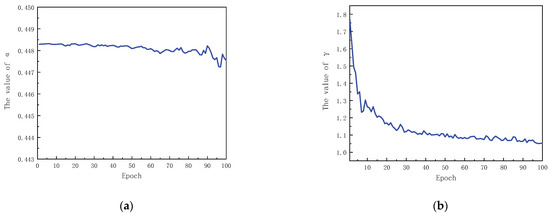
Figure 6.
Numerical dynamics of α and γ. (a) The numerical change process of α. (b) The numerical change process of γ.
Table 7 shows the comparison results between the method of dynamically changing weights proposed in this paper and the best results of multiple empirical values of Focal loss. It can be seen from Table 7 that the overall mAP value of the YOLOv5 model using the dynamic weight calculation method is higher than that of the empirical method.
Table 7.
Comparison of results from different valuation methods.
The mAP is increased by 0.3%, the accuracy and recall rate of defects remain similar to the empirical value method, and the detection accuracy and recall rate of insulators are increased by 1.2% and 0.7%, respectively. However, the dynamic value calculation method only needs one training to obtain an effect similar to the optimal value in the comparison results of multiple empirical values, which saves a lot of time and computing resources.
4.3. Comparison of Results of Other Algorithms
The comparison results of different algorithms are shown in Table 8. Compared with other different algorithms, Faster R-CNN has a higher recall rate for insulators and defects, but a lower detection accuracy. SSD has high accuracy for insulator and defect detection, but low recall. The mAP value of YOLOv3 is high, but the model volume is too large. The mAP value of YOLOv4 is close to YOLOv5, but the volume is slightly larger than YOLOv5. YOLOv5 achieves a balance of mAP and volume with the first four algorithms. Compared with Faster R-CNN, SSD, YOLOv3, YOLOv4, and YOLOv5, the improved algorithm proposed in this paper improves the overall mAP by 2.5%, 7.4%, 2.6%, 5.9%, and 5.7%, respectively. Our algorithms can especially improve the accuracy and recall rate of difficult-to-detect insulator defects.
Table 8.
Comparison of results from different algorithms.
4.4. Visualization of Experimental Results
In order to prove the real detection effect of the improved algorithm in this paper, the improved model is used for actual testing, as shown in Figure 7. The insulators are marked with a red frame, and the defects are marked with a pink frame. It can be seen from the visualization results that the model using the cross-entropy loss function has better detection ability and higher confidence for insulators, but no defects and small insulators are detected. The paper introduces a model of the Focal loss function, which reduces the confidence, but detects difficult defect parts and small insulators. It is proven that the model in this paper has a good detection effect on samples that are difficult to detect and classify.
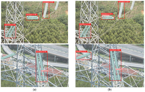
Figure 7.
Comparison chart of detection effects. (a) Use the cross-entropy loss function model to detect the effect. (b) Use the dynamically changing Focal loss function model to detect the effect.
5. Conclusions
In order to better detect the defects of transmission line insulators, this paper proposes an improved YOLOv5 model based on Focal loss. First, we use the CPLD data set and the National Grid Power’s inspection data to form a mixed data set, and then expand the data set through a variety of data enhancement methods. Secondly, transfer learning is performed with pre-training weights trained on large-scale data sets, which reduces the training time and improves the convergence speed of the model. Finally, the Focal loss function is introduced into the loss function and the weight factor is redesigned. The weight factor is dynamically updated according to the ratio of positive and negative samples in the feature diagram and the difference between the actual value and the predicted value in each training. By adjusting the loss function, the new algorithm increases the overall contribution of positive samples and difficult samples, makes the model more focused on insulator defects, and improves the model’s ability to detect insulator defects. From the experimental results, it can be concluded that the average accuracy of the algorithm in this paper can reach 98.3%, which is 5.7 percentage points higher than that of the original model, especially since the accuracy of defective insulators has been greatly improved.
Author Contributions
Conceptualization, Y.L. and G.Z.; methodology, Y.L.; software, Y.L.; validation, Y.L., G.Z. and S.A.; formal analysis, S.A.; investigation, G.Z.; resources, H.Z.; data curation, C.Z.; writing—original draft preparation, Y.L.; writing—review and editing, G.Z.; visualization, S.A.; supervision, C.Z.; project administration, G.Z. All authors have read and agreed to the published version of the manuscript.
Funding
This work was supported by the National Natural Science Foundation of China (No. 52077203) and the Fundamental Research Funds for the Provincial Universities of Zhejiang (No. 2021YW06).
Institutional Review Board Statement
Not applicable.
Informed Consent Statement
Not applicable.
Data Availability Statement
A part of the dataset is available at GitHub at: accessed on 1 July 2022. https://github.com/InsulatorData/InsulatorDataSet.
Conflicts of Interest
The authors declare no conflict of interest.
References
- Yang, L.; Fan, J.; Liu, Y.; Li, E.; Peng, J.; Liang, Z. A Review on State-of-the-Art Power Line Inspection Techniques. IEEE Trans. Instrum. Meas. 2020, 69, 9350–9365. [Google Scholar] [CrossRef]
- Nguyen, V.N.; Jenssen, R.; Roverso, D. Automatic autonomous vision-based power line inspection: A review of current status and the potential role of deep learning. Int. J. Electr. Power Energy Syst. 2018, 99, 107–120. [Google Scholar] [CrossRef]
- Ren, S.; He, K.; Girshick, R.; Sun, J. Faster r-cnn: Towards real-time object detection with region proposal networks. Adv. Neural Inf. Process. Syst. 2015, 39, 1137–1149. [Google Scholar] [CrossRef]
- Redmon, J.; Divvala, S.; Girshick, R.; Farhadi, A. You only look once: Unified, real-time object detection. In Proceedings of the Proceedings of the IEEE Conference on Computer Vision and Pattern Recognition, Las Vegas, NV, USA, 27–30 June 2016; pp. 779–788. [Google Scholar]
- Liu, W.; Anguelov, D.; Erhan, D.; Szegedy, C.; Reed, S.; Fu, C.-Y.; Berg, A.C. Ssd: Single shot multibox detector. In Proceedings of the European Conference on Computer Vision, Amsterdam, The Netherlands, 11–14 October 2016; pp. 21–37. [Google Scholar]
- Manninen, H.; Ramlal, C.J.; Singh, A.; Kilter, J.; Landsberg, M. Multi-stage deep learning networks for automated assessment of electricity transmission infrastructure using fly-by images. Electr. Power Syst. Res. 2022, 209, 107948. [Google Scholar] [CrossRef]
- Hosseini, M.M.; Umunnakwe, A.; Parvania, M.; Tasdizen, T. Intelligent Damage Classification and Estimation in Power Distribution Poles Using Unmanned Aerial Vehicles and Convolutional Neural Networks. IEEE Trans. Smart Grid 2020, 11, 3325–3333. [Google Scholar] [CrossRef]
- Liang, H.; Zuo, C.; Wei, W. Detection and Evaluation Method of Transmission Line Defects Based on Deep Learning. IEEE Access 2020, 8, 38448–38458. [Google Scholar] [CrossRef]
- Wanguo, W.; Zhenli, W.; Bin, L.; Yuechen, Y.; Xiaobin, S. Typical Defect Detection Technology of Transmission Line Based on Deep Learning. In Proceedings of the 2019 Chinese Automation Congress (CAC), Hangzhou, China, 22–24 November 2019; pp. 1185–1189. [Google Scholar]
- Zhao, Z.; Qi, H.; Qi, Y.; Zhang, K.; Zhai, Y.; Zhao, W. Detection Method Based on Automatic Visual Shape Clustering for Pin-Missing Defect in Transmission Lines. IEEE Trans. Instrum. Meas. 2020, 69, 6080–6091. [Google Scholar] [CrossRef]
- Qiu, Z.; Zhu, X.; Liao, C.; Shi, D.; Qu, W. Detection of Transmission Line Insulator Defects Based on an Improved Lightweight YOLOv4 Model. Appl. Sci. 2022, 12, 1207. [Google Scholar] [CrossRef]
- Zhang, Z.; Huang, S.; Li, Y.; Li, H.; Hao, H. Image Detection of Insulator Defects Based on Morphological Processing and Deep Learning. Energies 2022, 15, 2465. [Google Scholar] [CrossRef]
- Shrivastava, A.; Gupta, A.; Girshick, R. Training Region-Based Object Detectors with Online Hard Example Mining. In Proceedings of the 2016 IEEE Conference on Computer Vision and Pattern Recognition (CVPR), Las Vegas, NV, USA, 27–30 June 2016; pp. 761–769. [Google Scholar]
- Li, M.; Zhang, Z.; Yu, H.; Chen, X.; Li, D. S-OHEM: Stratified online hard example mining for object detection. In Proceedings of the CCF Chinese Conference on Computer Vision, Tianjin, China; 2017; pp. 166–177. [Google Scholar]
- Lin, T.Y.; Goyal, P.; Girshick, R.; He, K.; Dollár, P. Focal Loss for Dense Object Detection. In Proceedings of the 2017 IEEE International Conference on Computer Vision (ICCV), Venice, Italy, 22–29 October 2017; pp. 2999–3007. [Google Scholar]
- Li, B.; Liu, Y.; Wang, X. Gradient harmonized single-stage detector. In Proceedings of the AAAI Conference on Artificial Intelligence, Honolulu, HI, USA, 27 January–1 February 2019; pp. 8577–8584. [Google Scholar]
- Li, Y.; Liu, L. YOLO-ResNet: A New Model for Rebar Detection. In Proceedings of the 4th International Conference on Robotics, Control and Automation Engineering, RCAE 2021, Wuhan, China, 4–6 November 2021; pp. 128–132. [Google Scholar]
- Li, J.; Yan, D.; Luan, K.; Li, Z.; Liang, H. Deep Learning-Based Bird’s Nest Detection on Transmission Lines Using UAV Imagery. Appl. Sci. 2020, 10, 6147. [Google Scholar] [CrossRef]
- Li, Y.; Shi, W.; Liu, G.; Jiao, L.; Ma, Z.; Wei, L. Sar image object detection based on improved cross-entropy loss function with the attention of hard samples. In Proceedings of the 2021 IEEE International Geoscience and Remote Sensing Symposium, IGARSS 2021, Brussels, Belgium, 12–16 July 2021; pp. 4771–4774. [Google Scholar]
- Dai, G.W.; Fan, J.C. An Industrial-Grade Solution for Crop Disease Image Detection Tasks. Front. Plant Sci. 2022, 13, 921057. [Google Scholar] [CrossRef] [PubMed]
- Cao, C.-Y.; Zheng, J.-C.; Huang, Y.-Q.; Liu, J.; Yang, C.-F. Investigation of a Promoted You Only Look Once Algorithm and Its Application in Traffic Flow Monitoring. Appl. Sci. 2019, 9, 3619. [Google Scholar] [CrossRef]
- Liu, C.; Wu, Y.; Liu, J.; Sun, Z.; Xu, H. Insulator Faults Detection in Aerial Images from High-Voltage Transmission Lines Based on Deep Learning Model. Appl. Sci. 2021, 11, 4647. [Google Scholar] [CrossRef]
- Ultralytics/yolov5. Available online: https://github.com/ultralytics/yolov5 (accessed on 25 June 2020).
- Wang, C.Y.; Liao, H.; Wu, Y.H.; Chen, P.Y.; Yeh, I.H. CSPNet: A New Backbone that can Enhance Learning Capability of CNN. In Proceedings of the 2020 IEEE/CVF Conference on Computer Vision and Pattern Recognition Workshops (CVPRW), Seattle, WA, USA, 14–19 June 2020. [Google Scholar]
- Lin, T.Y.; Dollar, P.; Girshick, R.; He, K.; Hariharan, B.; Belongie, S. Feature Pyramid Networks for Object Detection. In Proceedings of the 2017 IEEE Conference on Computer Vision and Pattern Recognition (CVPR), Honolulu, HI, USA, 21–26 July 2017. [Google Scholar]
- Liu, S.; Qi, L.; Qin, H.; Shi, J.; Jia, J. Path Aggregation Network for Instance Segmentation. In Proceedings of the 2018 IEEE/CVF Conference on Computer Vision and Pattern Recognition (CVPR), Salt Lake City, UT, USA, 18–23 June 2018. [Google Scholar]
- Zheng, Z.; Wang, P.; Liu, W.; Li, J.; Ye, R.; Ren, D. Distance-IoU Loss: Faster and Better Learning for Bounding Box Regression. In Proceedings of the AAAI Conference on Artificial Intelligence, New York, NY, USA, 7–12 February 2020. [Google Scholar]
- Neubeck, A.; Gool, L. Efficient Non-Maximum Suppression. In Proceedings of the International Conference on Pattern Recognition, Hong Kong, China, 20–24 August 2006. [Google Scholar]
- Wang, Y.; Ma, X.; Chen, Z.; Luo, Y.; Yi, J.; Bailey, J. Symmetric Cross Entropy for Robust Learning with Noisy Labels. In Proceedings of the IEEE/CVF International Conference on Computer Vision, Seoul, Korea, 27 October–2 November 2019. [Google Scholar]
Publisher’s Note: MDPI stays neutral with regard to jurisdictional claims in published maps and institutional affiliations. |
© 2022 by the authors. Licensee MDPI, Basel, Switzerland. This article is an open access article distributed under the terms and conditions of the Creative Commons Attribution (CC BY) license (https://creativecommons.org/licenses/by/4.0/).