Abstract
The four-direction performance of a TOSA and power tested with different jumpers are affected by the optical field distribution of the TOSA. In order to improve the optical field distribution of a TOSA, this paper analyzes the factors affecting optical field distribution in the core and cladding of fiber and establishes a 3D defocusing coupling model to improve the uniform distribution of the optical field. The verification between the 2D coupling model and 3D defocusing coupling model shows that four-direction performance with 3D defocusing coupling is less than 1.0 dB, and the difference of power tested with different jumpers is not more than 0.5 dB. The results are better than that of a TOSA with a conventional coupling model, and the reliability and yield of the TOSA are higher. The 3D defocusing coupling model has practical guiding significance and economic value in TOSA production.
1. Introduction
Optical fiber communication technology has the characteristics of large capacity, high transmission quality, and good security. With the rapid development of optical fiber communication technology, it has become the irreplaceable communication technology in 4G and 5G networks and data center construction. As the core component in optical fiber communication networks, the optical module is mainly composed of optoelectronic components, functional circuits, and optical interfaces. Among them, optoelectronic devices include an optical emitting assembly (TOSA, transmitter optical sub-assembly) and an optical receiving assembly (ROSA, receiver optical sub-assembly), which performs the role of photoelectric conversion and electro-optical conversion. The TOSA converts the received electrical signal into the optical signal, and the optical signal is transmitted by the optical fiber. The TOSA is composed of a semiconductor laser diode (LD) and an optical fiber component through active coupling, and the ROSA is composed of a photodiode and an optical fiber component through active coupling [1].
The LD as a light source is used in a TOSA, and the beam emitted by the LD is shaped with a spherical or aspheric lens, and then coupled into the optical fiber. Usually, the appropriate coupling mode is selected according to the application requirements of the product and the requirements of coupling efficiency. Active coupling directly detects the optical power coupled into the optical fiber, but it cannot directly identify the distribution of the optical field in the optical fiber. If the distribution of the optical field is not uniform when the TOSA is tested with a jumper at different directions (four-direction performance) or tested with jumpers with different concentricity, the difference of optical power is large. Eventually, because of out of specification issues, the TOSA is not used as good product, which directly leads to product scrap and economic waste. The performance of the TOSA is affected by the coupling model, but there is little research on the coupling process at present [2,3,4,5,6,7,8]. Therefore, based on the study of factors affecting the distribution and optical simulation of the optical field in the fiber, this paper explores a coupling model that can improve the uniform distribution of the optical field. The three-dimensional (3D) defocusing coupling model entails the fiber moving up at the X/Y plane and coupling the maximum optical power, then moving up along the Z-axis with a step to change the optical power. At each step along the Z-axis, the fiber must couple the maximum optical power. When the optical power is the maximum, the optical energy in the core of fiber is the highest, and the energy distribution is the most uniform in the fiber core and cladding. The verification shows the optical power difference at four directions of the TOSA with the 3D defocusing coupling model within 1 dB, and the optical power difference tested by the jumper with different concentricity within 0.4 dB, which is better than the performance using two-dimensional (2D) coupling and 3D coupling. So, the 3D defocusing coupling model is a new coupling model for improving manufacturing efficiency and yield. This paper has important technical guiding significance and economic value as follows:
- (1)
- 3D defocusing coupling can guarantee the Gaussian distribution in the fiber without visual real-time monitoring.
- (2)
- The difference of a TOSA’s performance tested with different jumpers is small, which not only improves the yield of the TOSA, but also guarantee the performance of the optical module and client. At the same time, it reduces the technical requirements of the jumpers and directly reduces the cost of jumpers.
- (3)
- The 3D defocusing coupling model presented in this paper can be applied to other active-coupling products. In multi-mode coupling, the performance of circular flux in fiber can be improved, and the transmission performance of multi-mode products can be improved.
2. Analysis of the Influence of Optical Field Distribution in TOSA
2.1. Factors Affecting the Optical Field
LD beam quality and the TOSA coupling mode are the main factors affecting LD energy distribution in the single-mode fiber. Common parameters for evaluating LD beam quality include far-field the divergence angle, focal spot size, beam quality β factor, Strehle ratio, encircled energy ratio, M2 factor, etc. [9,10,11,12,13,14,15,16,17,18,19,20,21,22,23,24]. For a TOSA, the far-field divergence angle, focal spot size, and M2 factor are the main influencing factors.
The far-field divergence angle (θ) in the characteristic parameters of the Gaussian beam is defined as the angle corresponding to 1/e2 of the maximum intensity of the beam. When the laser transmits along the Z-axis, the far-field divergence angle (θ) is:
Equation (2) is substituted into Equation (1):
ω(z) is the beam width (beam radius) at the Z-axis, and ω0 is the waist radius. The far-field divergence angle represents the divergence of the beam. The larger the far-field divergence angle, the faster the beam diverges, the worse the quality of the beam, and the shorter the distance that the beam can transmit.
Focal spot size (ωƒ) refers to the size of the spot formed on the focal plane of the optical system after the laser beam passes through the focusing optical system. When the focal length of the focusing optical system is constant, the ωƒ is proportional to the far-field divergence angle (θ) of the measured beam. In this case, it is equivalent to using the size of the focal spot as the evaluation standard of the beam quality as the far field divergence angle. The larger the focal spot radius is, the larger the far field divergence angle is, and the worse the beam quality is. Taking the model in Figure 1 as a reference, the divergence angles θ⊥ is set as 15°, 20°, 25°, and 30°, respectively, and the corresponding RMS radius, geometric radius, and Airy spot radius were obtained by simulation, as shown in Table 1.
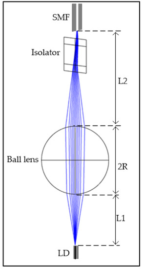
Figure 1.
Optical path model of TOSA.

Table 1.
Variation of far-field divergence angle and focal spot.
Beam quality β is defined as the ratio of the far-field divergence angle of the actual beam to the ideal far-field divergence angle. β is generally greater than 1. The closer to 1, the higher the beam quality is, and β = 1 is the maximum. β is mainly used to evaluate the laser beam emitted from the laser resonator, which can reasonably evaluate the near-field beam quality. It is a static performance index to describe the laser beam quality without considering the effects of atmospheric scattering, turbulence, and thermal halo.
The laser beam quality factor (M2) is defined as the product of the waist width of the actual beam and the far-field divergence angle divided by the product of the waist width of the fundamental mode Gaussian beam and the far-field divergence angle.
For the fundamental mode Gaussian beam:
In the formula, ω and ω0 are the waist widths of the actual beam and the fundamental mode Gaussian beam, respectively, and θ and θ0 are the far field divergence angles of the actual beam and the fundamental mode Gaussian beam, respectively.
Since the beam of the actual LD is not circular, there are large asymmetric far field divergence angles in transverse and lateral directions. The active layer of LD is relatively thin, so there is a larger divergence angle θ⊥ in the lateral direction, while there is a smaller divergence angle θ∥ in the transverse direction because of the wide active layer. Therefore, the M2 factor can be decomposed into transverse and lateral factors.
ω⊥ and ω∥ are the transverse and lateral beam waist widths, respectively.
The theoretical basis of the beam quality factor is the invariant principle of the product of beam waist width and far-field divergence angle. The beam waist width is determined by light intensity distribution on beam waist section, and the far-field divergence angle is determined by phase distribution. Therefore, M2, as a beam quality factor, can reflect the characteristics of intensity distribution and phase distribution of light field [25,26]. In order to achieve the coupling between LD and optical fiber, it is necessary to use an optical conversion element to transform the beam waist width and far-field divergence angle of LD, so that ωƒ can match the intrinsic mode field of single-mode fiber sufficiently.
2.2. Effect of Existing Coupling Model on the Distribution of Optical Field
A TOSA is composed of a LD TO (Transistor-Outline) -can, metal body, isolator and receptacle. The TO-can includes a tube cap with a lens, as shown in Figure 2. If the optical power of the TOSA is required to be relatively high, a tube cap with an aspherical lens is necessary [27,28,29,30]. The function of the lens is to transform the light emitted by the LD into convergent light, so that it can be more easily coupled into the fiber, as shown in Figure 1. In order to improve the optical return loss and reduce the influence of the optical reflection from the end-face of fiber to the LD, the end-face is usually processed into slop, and the angle of the slop is usually 2–8°. The angle is decided by the requirement of coupling efficiency and optical return loss. At present, the coupling process of TOSAs in the industry is mainly 2D and 3D coupling. As shown in Figure 3, optical power is the only monitored criterion.
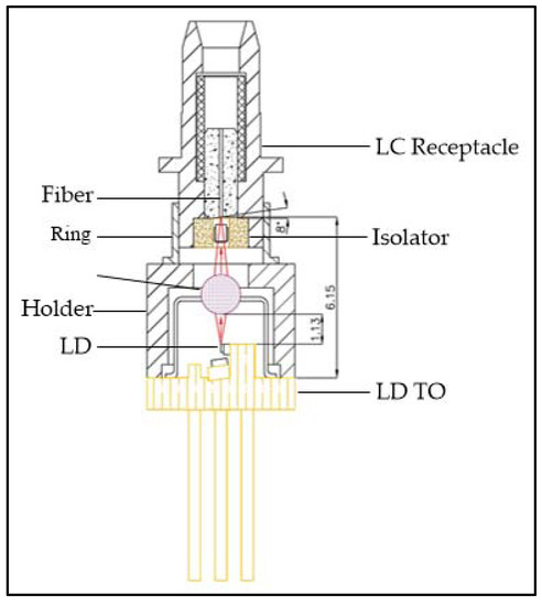
Figure 2.
Structure of TOSA.
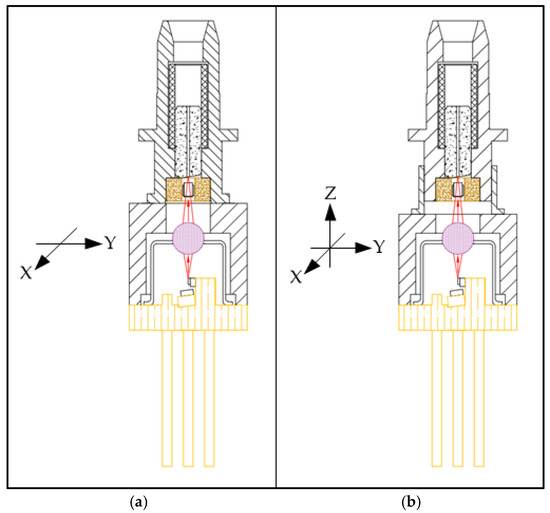
Figure 3.
Coupling model of TOSA. (a) 2D coupling model; (b) 3D coupling model.
Figure 3a is the schematic diagram of the 2D coupling model of the TOSA, and the receptacle is linked directly to the tube body, so the coupling process is very easy. The end-face of the receptacle is located on the focal plane of the LD TO, and the receptacle is moved up on the X/Y plane. The optical power changes by changing the relative position of the receptacle on the X/Y plane. At first, the receptacle is moved up to attain the highest optical power (Pmax). If the Pmax is within specification, the receptacle is stopped from moving. Conversely, if the Pmax is out of specification, the receptacle is moved up to reduce the optical power until the optical power is within specification. Finally, the receptacle and tube body are welded together using laser welding.
Figure 3b is the schematic diagram of the 3D coupling model, it has one more ring than the 2D model. The receptacle can be inserted into the ring smoothly, and the ring lays on the tube body. During coupling, the receptacle is moved up and the ring is driven to move on the X/Y plane, and the receptacle can be moved up along the Z-axis, but the ring still lays on the tube body.
In order to further illustrate the optical field distribution in 2D coupling, a simulation model is established based on the optical model in Figure 1. The optical field distribution in the core and cladding of the fiber after changing the relative position of the fiber and optical axis is shown.
Figure 4 is the distribution of the optical field in the fiber at the focal point of the LD TO. The X (μm) and Y (μm) represent the diameter of cladding, and (0,0) is the central point of the fiber core. The color represents the energy density. The optical field is mainly concentrated in the core and around the core, but the distribution is not uniform. This is because the end-face of fiber is not perpendicular to the central axis, which can cause the beam to segregate [27]. As shown in Figure 5, α is the inclination angle of the end-face, which is between the normal of the incident surface and the central axis; i represents the angle of incidence, i′ represents the angle of refraction into the core, and β represents the angle of segregation.
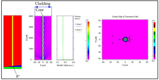
Figure 4.
Optical field distribution in fiber with 8° end-face at the focal position (0,0,0).
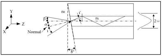
Figure 5.
Schematic diagram of the end-face with 8° of fiber.
Assuming that there is no off-axis and angular deflection for the fiber, the optical field distribution in the fiber can be shown as [28]:
The segregation angle is calculated according to the geometric-optical relationship of the optical total reflection in the fiber.
where n0 is the refractive index of air, n0 = 1, and n1 are the refractive index of the core, n1 = 1.468, α = 8°. After calculation, the value of β is approximately 3.76°. That is, when the incident beam is offset by 3.76° from the central axis of the fiber, the power coupled into the core of the fiber is the biggest and the coupling efficiency the highest.
Figure 6a–d show the distribution of the optical field in the core and cladding of fiber when the fiber moves up along the X-axis. It shows that more light is coupled into the cladding and the distribution in cladding is more irregular with increasing movement. Figure 6e–h show the distribution of the optical field in the core and cladding of fiber when the fiber moves up along the Y-axis. In Figure 6f, there is no discrete optical field in the cladding, which indicates that the incident angle of the end-face of the 8° fiber is consistent with the segregation angle when the fiber moves up 0.002 mm along the negative direction of the Y-axis, and the optical field is in the fiber core and around the fiber core. However, with the increasing movement along the positive direction of the Y-axis, the more optical field enters the cladding, and the distribution in the core and cladding is irregularity, which indicates that the incident angle is out of the segregation angle, and the light cannot be fully reflected inside the fiber core, so that the light is refracted into the cladding.
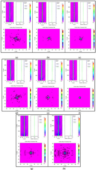
Figure 6.
The distribution of optical field with 8° fiber moving up along X/Y-axis. (a) is the optical fiber offset 4 μm along the negative X-axis, namely the coordinate (−0.004,0,0); (b) is the optical fiber offset 4 μm along the negative X-axis, namely the coordinate (−0.002,0,0); (c) is the optical fiber offset 2 μm along the positive X-axis, that is, the coordinate (0.002,0,0); (d) is the optical fiber offset 4 μm along the positive X-axis, namely the coordinate (0.004,0,0); (e) is the optical fiber offset 4 μm along the negative Y-axis, that is, the coordinate (0,−0.004,0); (f) is the optical fiber offset 2 μm along the negative Y-axis, that is, the coordinate (0,−0.002,0); (g) is the optical fiber offset 2 μm along the positive Y-axis, that is, the coordinate (0,0.002,0); (h) is the optical fiber’s positive Y-axis deviation of 4 μm, that is, the coordinate (0,0.004,0).
The focal position coordinates are set as (0,0,0), and the 8° optical fiber moves along the X-axis and Y-axis, respectively. The X (μm) and Y (μm) represent the diameter of cladding, and (0,0) is the central point of the fiber core. The color represents the energy density.
From the variation trend of the optical field in the fiber, the distribution of the optical field in the cladding is uneven when the fiber moves up along the X-axis or the Y-axis, which makes the power at four directions difference of the TOSA larger, and the power difference tested by jumpers with different concentricity larger also. Finally, the performance of the TOSA is out of specification under different testing conditions, and the yield of the TOSA is low.
3. Design of 3D Defocusing Coupling Model
Based on the 2D coupling model in Figure 3, the changing of coupling efficiency between 2D coupling and defocusing coupling is simulated, as shown in Figure 7. The light source in the simulation model is 10 G DFB TO from Mitsubishi, ML768K42T-91. The TO uses 1.5 mm ball lens, and the material is BK-7, n = 1.5. The fiber length in the receptacle is 4 mm, whose refractive index is 1.468, and the core diameter is 8.2 m with NA (Numerical Aperture) ~0.14. For 1310 nm, the mode field diameter is approximately 9.2 μm. The end-face angle of fiber is 8°.
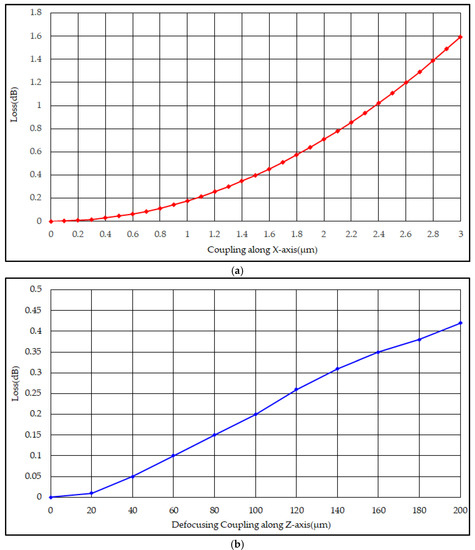
Figure 7.
Changing of coupling efficiency along X-axis and defocusing coupling. (a) is the changing tendency curve of optical loss based on 2D coupling model. The horizontal axis is the distance the end-face moving from (0,0) along positive direction of X-axis, and the vertical axis is the power loss that the power at focal point minus the power at X-axis; (b) is the changing tendency curve of optical loss based on defocusing coupling along Z-axis. The horizontal axis is the distance the end-face moving from (0,0) along positive direction of Z-axis, and the vertical axis is the power loss that the power at focal point minus the power at Z-axis.
Figure 7a shows that the coupling efficiency decreases rapidly when the TOSA uses the 2D coupling model, which can help to achieve target optical power within the specification fast. The X-axis represents the distance of the receptacle moving up from the optics axis along the X-axis, and the Y-axis represents the optical power loss with the receptacle moving up along the X-axis.
Figure 7b shows that the coupling efficiency decreases slowly when defocusing coupling along the Z-axis. The X-axis represents the distance of the receptacle moving up along the optics axis (positive Z-axis), and the Y-axis represents the optical power loss with the receptacle moving up along the optics axis.
From the above changing of the coupling efficiency, the 2D coupling model can improve the production efficiency of the TOSA. Therefore, the 2D coupling is favored by the designer and manufacturer of the TOSA. Even Figure 7b shows the 3D structure, the actual coupling process is 2D coupling, also. So, the distribution of the optical field in the fiber cannot be guaranteed, so that the power difference at four directions of the TOSA will be large, and the power difference tested by jumpers with different concentricity is relatively large also.
According to Equation (6), when the center of the laser beam light field coincides with the center of the fiber core, the optical field in the fiber is approximately a Gaussian distribution with the central line of the fiber core. The ideal coupling efficiency of the spherical lens is [30]:
ψO is the mode field distribution on the principal plane of the light emitted by the laser after passing through the ball lens, and ψF is the mode field distribution on the principal plane of the single-mode fiber. and are the complex conjugate distribution of the light source and the single-mode fiber on the principal plane, respectively. For single-mode fiber, the mode field radius of 1310 nm is 4.6 um. The coupling efficiency is the highest when ψO is closest to ψF. Conversely, the highest the coupling efficiency is, the best ψO matches ψF.
According to the relationship between the optimal coupling efficiency and the optical field, in order to guarantee the uniform distribution of the optical field in the fiber, the TOSA must be coupled to the maximum optical power on the optical plane, that is, the coupling efficiency must be highest. In this paper, a 3D defocusing coupling model for a TOSA is established. The structure of the TOSA is shown in Figure 7b. Before coupling, the LC receptacle is linked to a power meter using fiber jumpers, and the power value is associated with the coordinate of the end-face of fiber. The end-face of fiber is moved up the X/Y plane and along the Z-axis with the power changing.
For the first step, the end-face of fiber is placed near the focal point of the LD TO and moved up with coarse step on the X/Y plane before the power meter reads the optical power through the fiber jumper. Once a little optical power value (P1) is read at some coordinate, this coordinate point (X1, Y1) is as a dot.
The second step, the end-face of fiber is move up with fine step within radius 0.5 mm or smaller. The highest optical power (P2) and the coordinates (X2, Y2) are obtained in this range.
The third step, the end-face of fiber is moved up a fine step along the positive Z-axis and then repeats the first and the second steps. The highest optical power (P3) and the coordinates (X3, Y3) are obtained in the plane. If P3 > P2, the end-face of fiber is moved up a fine step along the positive Z-axis again and repeated the first step and the second step. Then, the optical power (P4) is compared with P3. If P4 > P3, the third step is repeated until the optical power (Pmax) is the highest. When the Pmax is within the specification of optical power, the receptacle is welded with a ring using laser welding, then the ring is welded on the body. If the Pmax is out of specification, the third step is repeated until the optical power is within the specification.
Conversely, if P3 < P2, the end-face of fiber is moved up along the negative Z-axis, and repeated the first step and the second step. Then, the power (P5) is compared with P3. If P5 > P3, the end-face of fiber is moved up a fine step along the positive Z-axis again, and repeated the first step and the second step until the optical power (Pmax′) is the highest. When the Pmax is within the specification of optical power, the receptacle is welded with a ring by laser welding, then the ring is welded on the body. If the Pmax is out of specification, the step is repeated until the optical power is within the specification.
Figure 8 shows an optical simulation of the 3D defocusing coupling. When the end-face of fiber is at the focal point, the optical field is mainly concentrated in and around the core, and there is only little stray light in the cladding, which is caused by the 8° end-face of fiber. When the fiber moves up 60 μm along Z-axis, there is some light in the cladding, but the optical field is distributed hierarchically around the central axis of the fiber. When the fiber moves up to 120 μm, there is more optical energy in the cladding. Compared with the distribution of the optical field in the fiber with 2D coupling, the distribution in the fiber with 3D defocusing coupling is more uniform and symmetrical.
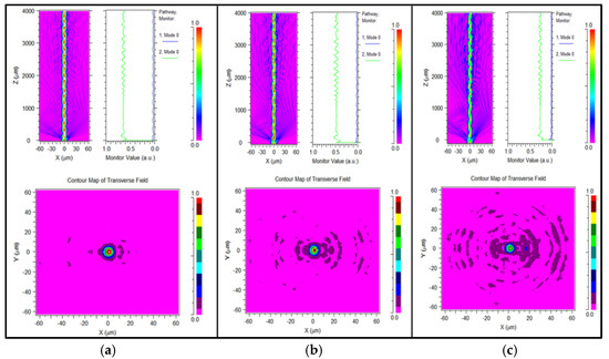
Figure 8.
The optical field distribution of fiber moving up in Z-axis. (a) is the distribution of optical field when the end-face of fiber is at the focal point of the LD TO, Z = 0 μm. (b) is the distribution of optical field at the maximum power where the fiber moves up 60 μm along Z-axis, Z = 60 μm. (c) is the distribution of optical field at the maximum power where the fiber moves up 120 μm along Z-axis, Z = 120 μm.
4. Verification of 3D Defocusing Coupling Model
4.1. Designing of Model
The LD TO is 10 G DFB ML768K42T-91 from Mitsubishi, and the TO is welded onto a stainless body with energy storage welding. The adapter is an XMD (10 Gbit/s Miniature Device) -type receptacle with SMF-28e fiber. A single-stage free-space isolator is assembled in the receptacle. After coupling with the LD TO, the receptacle is welded onto the body through the stainless ring. Then, the TOSA is completed (see Table 2).
Table 2.
Parameters of TOSA.
The 2D and 3D beam quality of a set of LD TO is tested by a slit sweep beam quality analyzer, as shown in Figure 9 and Figure 10. The test data are shown in Table 3.
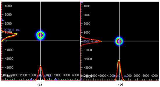
Figure 9.
Beam quality of 2D. The horizontal axis and the vertical axis are the spatial coordinates of the 2D beam analyzer, and the (0,0) is the central point. The horizontal axis represents the direction of θ∥, and the vertical axis represents the direction of θ⊥. The color represents the energy. (a) is the beam quality of 2D with the central point offsetting (0,0) because the chip is bonded within the tolerance. (b) is the beam quality of 2D without the central point offsetting.
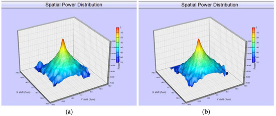
Table 3.
Data of beam quality.
From the beam quality data, the Gaussian diameter after converging through the lens is relatively large, mainly because of the large divergence angle of the LD and the large aberration caused by the ball lens. Besides, the accuracy of the TO-can package between the laser and the ball lens affects the Gaussian diameter also. The large Gaussian diameter eventually makes coupling efficiency lower. The theoretical coupling efficiency is 14% with PC fiber coupling the TO, while the coupling efficiency is 12.5% when the fiber is APC (Angled Physical Contact). IEEE Std 802.3 CA defines −8.2~0.5 dBm (0.15~1.13 mW) as the output power of the transmitter for a 10 G 10 km optical module, so the output power of the LD TO is >3.6 mW @Ith +20 mA, and 5% is enough for the coupling efficiency. Therefore, an appropriate coupling mode is very important for the performance of a TOSA.
Based on the two coupling models in this paper, 50 pcs samples are made by using IEC61755-3-1 Class B fiber jumper. First, as shown in Figure 3a, the end-face of the receptacle is at the focal point of the TO, and only two-dimensional coupling is performed in the X/Y plane. When the optical power is within −8.2~0.5 dBm, the receptacle is weld on the body using laser welding. Second, as shown in Figure 3b, 3D defocusing coupling is used. The maximum power is found in the X/Y plane, then the power is adjusted by moving up the receptacle along the Z-axis step by step. When the optical power is within −8.2~0.5 dBm, the receptacle is welded on the ring. The receptacle with the ring moves up on the body to couple maximum power, then is welded on the body.
4.2. Data Analysis
A Class B jumper with a 1.12 μm concentricity and a Class C jumper with 1.46 μm concentricity are used to test the four-direction performance of the TOSA, respectively. The TOSA is fixed, and the jumper is rotated along the directions of 0°, 90°, 180°, and 270° to test the optical power. The difference between the maximum optical power and the minimum optical power is the four-direction performance, and the unit is dB.
Figure 11a shows the four-direction performance of the TOSA with a 2D coupling model, which is shown in Figure 10a. During coupling, the optical power changes by moving up the receptacle in the X/Y plane. The four-direction performance of TOSA samples is tested with the Class B and Class C jumper, respectively. The blue curve represents four-direction performance tested with the Class B jumper, and the red curve represents the four-direction performance tested with the Class C jumper. From the distribution of data, the minimum value is 0.3 dB and the maximum is 3.1 dB. The distribution range is relatively large, and the four-direction performance tested with the Class B jumper is not significantly better than that tested with the Class C jumper. It indicates that the light in the core and cladding of a TOSA with 2D coupling model is not uniform or in approximate Gaussian distribution, but in discrete distribution. When a jumper with a different concentricity is used to test the four-direction performance, the light in the core and cladding of the TOSA cannot completely enter the core and cladding of the jumper at different direction, resulting in a large difference of optical power.
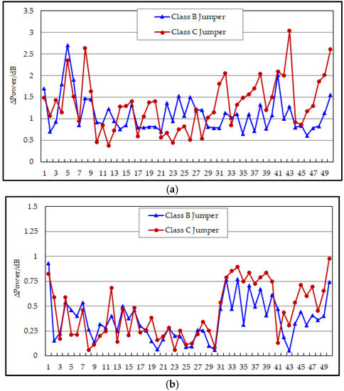
Figure 11.
(a) is the distribution of four-direction data with 2D coupling model. (b) is the distribution of four-direction data with 3D defocusing coupling model. The horizontal axis represents the serial number of samples, and the vertical axis represents the power changing.
Figure 11b shows the four-direction performance of the TOSA with a 3D defocusing coupling model, as shown in Figure 3b. The four-direction performance is tested with Class B and Class C jumpers as mentioned above. The blue curve represents the result with the Class B jumper, and the red curve represents the result with the Class C jumper. From the data distribution, there is a small difference in the four-direction performance between the Class B jumper and Class C jumper, and the difference is <0.5 dB. It is deduced that the light in the core and cladding of the TOSA is near Gaussian distribution, and most of the light concentrates in and around the core. Even though the concentricity of the jumper is different, the light enters into the core, so that the four-direction performance is good.
Furthermore, these samples are tested at 0° direction with 2 pcs Class B jumpers, whose concentricity is 0.42 μm and 0.97 um, and also with 2 pcs Class C jumpers, whose concentricity is 1.38 μm and 1.42 um. The difference between maximum and minimum optical power was compared.
Figure 12a shows the difference of the optical power tested with Class B and Class C jumpers when the TOSA has 2D coupling. The blue curve represents the distribution of the optical power difference tested with 2 pcs Class B jumpers, and the average difference is approximately 0.5 dB. The red curve represents the distribution of the optical power differences tested with 2 pcs Class C jumpers, and the maximum difference is approximately 1.8 dB. Comparing the distribution, the difference of optical power tested with the Class C jumper is larger than that tested with the Class B jumper.
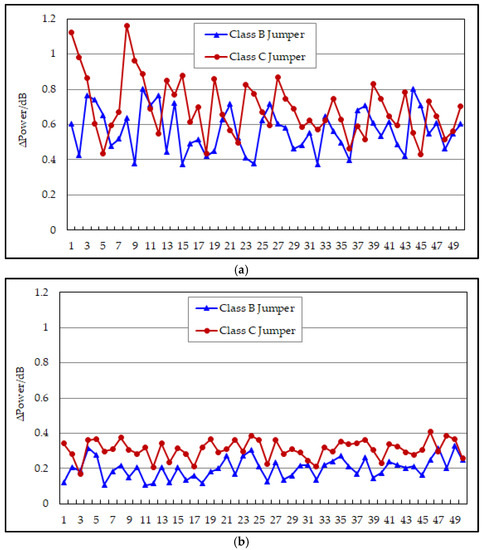
Figure 12.
(a) is the data of TOSA with 2D coupling tested with different jumpers. (b) is the data of TOSA with 3D defocusing coupling tested with different jumpers. The horizontal axis represents the serial number of samples, and the vertical axis represents the power changing.
Figure 12b shows the difference of the optical power tested with Class B and Class C jumpers, and these samples use 3D defocusing coupling. The blue curve represents the distribution of the optical power difference tested with 2 pcs Class B jumpers, and the red curve represents the distribution of the optical power difference tested with 2 pcs Class C jumpers. Both curves show that the difference of optical power and fluctuation between Class B and Class C jumper is small, and the difference of optical power tested with the Class C jumper is less than 0.4 dB. Comparing the curves shown in Figure 12a,b, whether these samples are tested with Class B jumpers or Class C jumpers, the changing of optical power with 3D defocusing coupling is significantly smaller than that with 2D coupling.
From the analysis and verification, it shows that the distribution of light in the core and cladding of fiber is decided by the coupling model of the TOSA, which eventually affects the performance of the TOSA. The 3D defocusing coupling model can effectively improve the performance of a TOSA.
5. Conclusions
The factors impacting the distribution of an optical field in fiber is analyzed comprehensively, and the model of 3D defocusing coupling improving the Gaussian distribution of optical filed is established. Two groups of TOSA samples with 3D defocusing coupling and 2D coupling are completed, and the four-direction performance and difference of optical power with different jumpers are tested. Four-direction performance with 3D defocusing coupling is <1 dB, and the difference of optical power with different jumpers is <0.5 dB. Comparing the performance of a TOSA with traditional 2D coupling, the performance of the TOSA with 3D defocusing coupling is better than that with 2D coupling significantly. So, as active coupling, the 3D defocusing coupling model can help to improve the yield and final performance of a TOSA, and it can be used for other optical devices. In the next step, the influences of temperature on and the refractive index of the lens on the optical field will be studied, and a comprehensive factors and model for an optical fiber active device will be established.
Author Contributions
Methodology, X.D.; Project administration, S.D.; Validation, J.J. All authors have read and agreed to the published version of the manuscript.
Funding
This research was funded by Key Scientific Research Projects of Colleges and Universities in Henan Province (Grant No. 23A520054) and International training project of high level talents in Henan Province.
Institutional Review Board Statement
Not applicable.
Informed Consent Statement
Not applicable.
Data Availability Statement
Not applicable.
Conflicts of Interest
The authors declare no conflict of interest.
References
- Kerser, G. Optical Fiber Communications, 3rd ed.; Publishing House of Electronics Industry: Beijing, China, 2002; pp. 161–169. [Google Scholar]
- Jing, Y.; Zheng, J. Research progress of fiber coupled technology for side emission semiconductor laser. Chin. J. Quantum Electron. 2019, 36, 641–650. [Google Scholar]
- Ellis, S.C.; Bland-Hawthorn, J.; Leon-Saval, S.G. General coupling efficiency for fiber-fed astronomical instruments. J. Opt. Soc. Am. B. 2021, 38, a64–a74. [Google Scholar] [CrossRef]
- Guo, Z.-S.; Qin, W.-B.; Li, J.; Liu, Y.-Q.; Cao, Y.-H.; Meng, J.; Guan, J.-Y.; Pan, J.-Y.; Lan, T.; Li, Q.-X.; et al. Fiber Coupling of Semiconductor Laser Based on Wedge-shaped Lens. Chin. J. Lumin 2021, 42, 98–103. [Google Scholar] [CrossRef]
- Forrer, M.; Strub, H.; Honig, T.; Koller, N.; Kunz, A.; Moser, H.; Brecher, C.; Hoeren, M.; Zontar, D. High precision automated tab assembly with micro optics for optimized high-power diode laser collimation. SPIE Photonics West. 2020, 11261, 112610B. [Google Scholar]
- Yang, X.; Jiao, Q.; Wang, Y. Evaluation of beam quality of semiconductor lasers by beam parameter product. Laser Technol. 2018, 42, 859–861. [Google Scholar]
- Cai, J.; Li, S. Analysis and Measurement of Beam Quality of Quantum Cascade Laser. Electro-Optic Technol. Appl. 2018, 33, 13–16. [Google Scholar]
- Chang, Y.; Liu, Z. Performance analysis of an all-optical double-hop free-space optical communication system considering fiber coupling. Appl. Opt. 2021, 60, 5629–5637. [Google Scholar] [CrossRef]
- Jung, A.; Song, S.; Kim, S.; Oh, K. Numerical analyses of a spectral beam combining multiple Yb-doped fiber lasers for optimal beam quality and combining efficiency. Opt. Exp. 2022, 30, 13305–13319. [Google Scholar] [CrossRef]
- Tong, Y.; Shang, J. Surface quality of laser paint removal of marine steel: A comparative study using a Gaussian beam and a flat-top beam. Appl. Opt. 2022, 61, 2237–2246. [Google Scholar] [CrossRef] [PubMed]
- Du, M.; Loetgering, L.; Eikema, K.S.; Witte, S. Measuring laser beam quality, wavefronts, and lens aberrations using ptychography. Opt. Exp. 2020, 28, 5022–5034. [Google Scholar] [CrossRef]
- Li, S.; Du, P. Study of evaluating nearfield beam quality of the high power laser beams. Optik 2018, 157, 148–155. [Google Scholar] [CrossRef]
- Han, K.; Cui, W.; Yang, Y.; Xi, F.; Li, X.; Du, S. Evaluating the Potential of Laser Beam Quality Improvement by Adaptive Optics System. Int. J. Opt. 2019, 2019, 1970406. [Google Scholar] [CrossRef]
- Ma, Z.; Jiang, L.; Zhou, J.; Yang, J. Simulation study for the influence of laser-emitting system on beam quality. Proc. SPIE 2019, 11023, 110233O. [Google Scholar]
- Hou, G.; Wang, L.; Feng, J.; Popp, A.; Schmidt, B.; Lu, H.; Tong, C.; Shu, S.; Wang, L. Near-diffraction-limited semiconductor disk lasers. Opt. Commun. 2019, 449, 39–44. [Google Scholar] [CrossRef]
- Lin, J.; Zeng, X.; An, Y. A Method for Evaluating Beam Quality of Laser Diode. Chin. J. Quantum Electron. 2005, 22, 550–553. [Google Scholar]
- Zhang, X.; Cao, Y. Research on the beam quality of diode lasers based on Wigner distribution function. In Proceedings of the International Conference on Photonics and Optical Engineering, Xi’an, China, 5–8 December 2018; p. 11052. [Google Scholar]
- Cao, C.; Wang, X. The problem with beam quality for semiconductor laser. Optik 2016, 127, 3701–3702. [Google Scholar]
- Pan, S.; Ma, J. Real-time complex amplitude reconstruction method for beam quality M2 factor measurement. Opt. Exp. 2017, 25, 20142–20155. [Google Scholar] [CrossRef] [PubMed]
- Scholes, S.; Forbes, A. Improving the beam quality factor (M2) by phase-only reshaping of structured light. Opt. Lett. 2020, 45, 3753–3756. [Google Scholar] [CrossRef] [PubMed]
- Mahdieh, M.H.; Jafarabadi, M.A.; Ahmadinejad, E. Thermal lens effect induced by high power diode laser beam in liquid ethanol and its influence on a probe laser beam quality. SPIE 2015, 9255, 925531. [Google Scholar]
- Lv, B.; Ji, X.; Luo, S.; Tao, X. Parametric Characterization of Laser Beams and Beam Quality. Infrared Laser Eng. 2004, 33, 14–17. [Google Scholar]
- Sun, F.; Zhao, Y. High beam quality broad-area diode lasers by spectral beam combining with double filters. Chin. Opt. Lett. 2019, 14, 011401. [Google Scholar]
- Fu, S.; Pan, Y. Designing a high-efficiency coupling system to couple a hollow Gaussian beam into single-mode fiber. Appl. Opt. 2021, 60, 10617–10624. [Google Scholar] [CrossRef]
- Li, W.; Chen, J. Design and Optimization of a Single-mode Fiber Double Gaussian Coupling Lens. Vac. Cryog. 2021, 27, 400–406. [Google Scholar]
- Bouhafs, Z.; Guessoum, A.; Guermat, A.; Bouaziz, D.; Lecler, S.; Demagh, N.-E. Parabolic microlensed optical fiber for coupling efficiency improvement in single mode fiber. Opt. Contin. 2022, 1, 1218–1231. [Google Scholar] [CrossRef]
- Karstensen, H. Laser Diode to Single-Mode Fiber Coupling With Ball Lens. Opt. Commun. 1988, 9, 42–49. [Google Scholar]
- Richard, A.; Schwarz, D.A. Ball lens coupled fiber-optic probe for depth-resolved spectroscopy of epithelial tissue. Opt. Lett. 2005, 30, 1159–1161. [Google Scholar]
- Hu, Q.; Long, W. The effect of lateral deviation on coupling efficiency of fiber connector and its compensation method. J. Opt. 2019, 48, 461–467. [Google Scholar] [CrossRef]
- Zhang, F.; Zheng, Y. Coupling efficiency between ball lens capped laser diode chip and single mode fiber. Optik 2018, 157, 497–502. [Google Scholar] [CrossRef]
Publisher’s Note: MDPI stays neutral with regard to jurisdictional claims in published maps and institutional affiliations. |
© 2022 by the authors. Licensee MDPI, Basel, Switzerland. This article is an open access article distributed under the terms and conditions of the Creative Commons Attribution (CC BY) license (https://creativecommons.org/licenses/by/4.0/).