A Novel Convolutional Adversarial Framework for Multivariate Time Series Anomaly Detection and Explanation in Cloud Environment

Abstract

Anomaly detection is critical to ensure cloud infrastructures’ quality of service. However, due to the complexity of inconspicuous (indistinct) anomalies, high dynamicity, and the lack of anomaly labels in the cloud environment, multivariate time series anomaly detection becomes more difficult. The existing approaches are rarely effective in meeting these challenges. In this paper, we propose a novel convolutional adversarial model, convolutional-adversarial-training-based integrated anomaly detection with explanation framework (CAT-IADEF), for multivariate time series anomaly detection in the cloud. We adopt three convolutional neural networks to learn sequence features and adversarial training to amplify “slight” anomalies while enhancing the robustness of the model. The dynamic threshold is determined in real time by the peaks over threshold (POT) method to improve detection accuracy. In addition, anomaly explanation is also conducted efficiently by analyzing anomaly score vectors. Experiments with seven data subsets from various public datasets show that CAT-IADEF outperforms state-of-the-art methods. The average F1 score on the seven datasets is 0.907, which is 6.5% higher than the state-of-the-art model and up to 22.1% higher than the baseline method. Furthermore, the proposed anomaly explanation framework is also integrated into various models to verify its effectiveness on the experimental datasets.

1. Introduction

Cloud computing has evolved from a set of promising virtualization and data center technologies to a consolidated paradigm for delivering computing as a service to end customers. Moreover, it has mighty computing power, allowing users to access and execute cloud computing in various ways and quickly provide resources based on their needs [1].

However, with the drastic increase in data volume and network application scope, the deployment of the cloud platform is increasing, and vast amounts of data need to be processed, all of which require the reliability of cloud computing systems [2]. This means that the cloud computing system needs to perform anomaly detection of time series data, detect anomalies, and give possible reasons or circumstances for the occurrence of anomalies. In the initial stages, researchers proposed a univariate time series anomaly detection method that analyzed system metrics, such as the number of I/O requests, memory usage, throughput, etc. However, with the increasing complexity of cloud systems, there are now multiple time series for cloud performance monitoring data. For example, when monitoring the abnormal state of the CPU, it is necessary to collect the percentage of user space occupied by the CPU, the CPU idle rate, and the percentage of CPU time waiting for input and output as well as different aspects of data, such as the total percentage used by the CPU. In addition, the traditional methods significantly impact performance due to the increase in sizes, so anomaly detection of multivariate time series has become a research hotspot [3].

Traditional anomaly detection methods, such as setting a static threshold, determined that a certain observed data point exceeded the set threshold to be an outlier point. Collecting data with many labels is complicated by the increase in data scale, which results in a lack of time series data, lack of branding, and other problems. In addition, the detection of the “slight” anomalies proposed in unsupervised anomaly detection (USAD) [4] and the stability of training are also current priorities to consider. To facilitate further research, anomaly explanation is defined in this paper as the dimensions of the most likely occurrence of anomalies. We propose an adversarial training method for anomaly explanation. Firstly, we use convolutional neural networks (CNN) to extract the sequence’s main features. Next, we build an adversarial training architecture consisting of three CNNs combined with the POT dynamic threshold selection. Then, we also add the anomaly explanation module based on the anomaly attribution matrix calculation for each point.

The contributions of this paper include the following:

• To solve the problem that “slight” anomalies are not easy to identify as well as the detection model’s robustness, we adopt adversarial training to amplify the reconstruction errors for anomaly identification while improving the model’s accuracy.
• To improve the computational efficiency of static threshold exploration, we combine the POT dynamic threshold selection technology effectively to improve the detection performance.
• To effectively support anomaly handling afterward, we propose an anomaly explanation framework. First, based on each point’s anomaly score and threshold matrix, we calculate the number of anomalies to perform anomaly dimension attribution, which explains the anomalies to a certain extent.

The organization of this paper is as follows: The Section 1 mainly introduces the research background, purpose, and significance and briefly analyzes the anomaly detection problems. The Section 2 briefly reviews the classical anomaly detection methods, deep learning-based anomaly detection methods, and anomaly explanation methods. The Section 3 details the adversarial convolutional neural network model proposed in this paper. The Section 4 validates the model’s overall performance and analyzes the results accordingly. At the same time, ablation experiments are carried out to investigate the influence of each component of the model on its overall performance. Finally, the Section 5 summarizes the presented models and provides potential future work.

2. Related Work

We briefly review the existing anomaly detection work, especially recent progress in multivariate time series anomaly detection and anomaly explanation. First, we start with the classical anomaly detection methods; then, we move on to the deep learning-based anomaly detection method and anomaly explanation method. More comprehensive literature reviews can be found in recent surveys [5].

2.1. Classical Anomaly Detection Methods

In the field of anomaly detection, there are some classic methods. For example, 3sigma identifies anomalies by measuring whether current values deviate from historical averages and whether deviations meet three standard deviations. The principal component analysis (PCA) [6] method uses the weight of the eigenvalue to calculate the eigenvector distance difference corresponding to the sample point’s eigenvalue so as to calculate the deviation degree of the data value from this direction. It identifies abnormalities based on the accumulation of the deviation degree for each order. The distance-based method of K-nearest neighbors (KNN) [7] determines an anomaly when the average distance of the K-nearest neighbors is more significant than the threshold. Copula-based outlier detection (COPOD) [8] uses statistical probability functions to calculate the left and right tail probabilities. It outputs the most suitable tail probabilities according to the specific situation to perform anomaly detection. Its advantages are that it does not need to calculate the distance of the sample parts, the overhead is small, and no parameter adjustment is required. The local outlier factor (LOF) [9] method is a density-based unsupervised anomaly detection method that assigns each data point an LOF dependent on the density of the neighborhood and then compares each point to the corresponding field density to determine whether the data point is an outlier, similar to the density-based connectivity-based outlier factor (COF) [10]. One-class support vector machines (OCSVM) aim to learn decision boundaries [11,12] for normal observations while taking some outliers into account. If the data is two-dimensional, it is to find a hyperplane to divide the normal data and some outliers, and if it is multi-dimensional data, it is to find a surface to divide. The anomalies are identified by observing whether a data point falls within the decision boundary. Ref. [13] studies various machine learning approaches for informational/noninformational classifications. A robust random cut forest (RRCF) improves the isolation forest algorithm (IF) by integrating ideas to process streaming data [14,15,16].

The simplicity of the classical method has always been its advantage, but it has limitations when dealing with nonlinear, high-dimensional, and noisy data.

2.2. Methods Based on Deep Learning

The methods based on deep learning usually build some complex deep neural network frameworks. The most common auto-encoder (AE) is to compress and reconstruct data to obtain reconstruction losses and to judge anomalies by reconstruction loss. The variation auto-encoder (VAE) [17,18] is a stochastic generative model that provides calibrated probabilities computed by reconstructing the probability density. The long short-term memory-based variational auto-encoder (LSTM-VAE) [19] aims to replace the feedforward network in VAE with LSTM [20,21].

Some newer methods, such as the multivariate anomaly detection with GAN (MAD_ GAN) framework [22,23], have a basic architecture similar to the previous generative adversarial network (GAN) [24]. MAD_GAN adopts a long- and short-term recurrent neural network as the basic model of GAN learning to analyze time-dependent multivariate time series data. Its advantage is that it does not need to introduce a lower bound for likelihood estimation and only performs anomaly detection by modeling the nonlinear associations between multiple time series. OmniAnomaly [25] proposes a stochastic recurrent neural network that establishes an explicit time dependency between random variables and uses a stochastic recurrent neural network and a planar normalized flow to generate reconstruction probabilities. It also proposes a method for dynamically selecting the threshold (POT). Ref. [26] leverages a novel threshold to detect cyber attacks. USAD [4] improves the basic AE, adds a decoder, processes the sequence data through three simple auto-encoders, and judges the abnormality based on the reconstruction error; however, the most basic linear changes sometimes cannot effectively extract sequence features. The multivariate time series anomaly detection via graph attention network framework (MTAD-GAT) builds the model jointly by combining the prediction and reconstruction methods using a graph attention network to model the feature and temporal correlation [27]. The deep transformer network for anomaly detection (TranAD) model [28] is a typical representative of anomaly detection combined with a transformer. It uses an attention mechanism to learn temporal trends and model-agnostic meta-learning to guarantee its performance even with limited datasets. It still judges anomalies by the reconstruction error.

2.3. Anomaly Explanation Method

After anomaly detection, the focus of researchers’ concern has been how to interpret the detected anomaly. The multi-scale convolutional recurrent encoder–decoder (MSCRED) [29] uses different channel widths to capture short-, medium-, and long-term anomalies. HitRate@P% is used in OmniAnomaly [25] to measure the diagnostic performance of the model. TranAD [28] adds the normalized discount cumulative NDCG@P% on this basis. Bayesian networks are proposed in [30] to perform causal relationship detection for multiple networks and the physical features of a system. Finally, an unsupervised approach is used in [31] to reduce the anomaly feature space to isolate anomalies continuously.

The anomaly detection methods, as mentioned earlier, have good detection performances. However, their performances across different time series datasets are inconsistent (limited ability to set or identify “slight” anomalies using only static thresholds), and their performances in anomaly explanation are inadequate. In addition, anomalies are explained in methods that do not intuitively give the most likely dimensions of an anomaly for researchers to use. To address these issues, the CAT-IADEF model combines CNN adversarial training and the POT dynamic threshold selection, enabling the model to identify “slight” anomalies while improving its stability and detection performance. Further anomalies are also carried out in the Anomaly Explanation section.

3. Method

We formalize the research issues in Section 3.1 and detail our research methods in Section 3.2, Section 3.3, Section 3.4 and Section 3.5.

3.1. Problem Statement

A time series refers to a sequence formed by arranging the values of a particular statistical indicator of a specific phenomenon at different times in chronological order. In a single-variable time series, such as $T=\{x_1,x_2,\cdots x_t\}$, a series of data is collected over time, and the entire series contains only one variable. For a multivariate time series, such as $T=\{x_1,x_2,\cdots x_t\}$, there is $x_t=[h_{1t},h_{2t}\cdots h_{kt}]$. The significance of anomaly detection and anomaly explanation in this study is as follows: Regarding anomaly detection, we first normalize the maximum and minimum values for any time series T. Then, we define a time window $Wt=\{x_{t-k+1},\cdots x_{t-1},x_t\}$ of the length k at time t and convert the time series T into a window series $W=\{W_1,W_2\cdots W_T\}$.

We use the window series W as the training input to construct the Y; first, we calculate the reconstruction loss $L_t$. Next, we calculate the abnormal score $S_t$ and then calculate a threshold $threshold$ based on the quirky score of the previous window. For regular data points, we assume that they can be well reconstructed. For anomalies, the reconstruction error is calculated to compare with the threshold, so a label $y\in (0,1)$ can be obtained. Regarding anomaly explanation, for any time series T, we calculate the reconstruction loss of all data points and, based on this, predict a label sequence data, $Y=\{y_1,y_2\cdots y_t\}$, composed of $y_t\in (0,1)$ so that the sequence dimension with the most ones can be calculated.

3.2. Overall Architecture of CAT-IADEF

As shown in Figure 1, three CNN models make up the overall CAT-IADEF framework.

First, on the left side of the figure is the window sequence W obtained by processing the time series data T, which is input into the convolutional auto-encoder to obtain a set of latent variables Z. Afterward, in the middle of the figure, two sets of auto-encoders $E{D}_1$ and $E{D}_2$ (the two decoders are composed of encoders, respectively) are trained adversarially to enhance the $E{D}_2$ model’s ability to identify “slight” anomalies and output the reconstructed data of the two auto-encoders during the adversarial training phase. By calculating the reconstruction loss L of the two sets of auto-encoders and performing a weighted average to obtain the anomaly score $S_i$, it is possible to then perform anomaly detection on a multivariate time series. Finally, on the right side of the figure is the anomaly interpretation module, which inputs the anomaly score for each data point and stores it in the label matrix R by comparing it with a threshold and assigning it a value of 0 or 1. The matrix R sums each column, and the column with the largest value represents the dimension with the most ones, which is the dimension where the anomaly is most likely to exist.

3.3. CNN-Based Adversarial Training

GAN-style adversarial training methods have been shown to perform well in anomaly detection on time series data [24]. To this end, we also constructed two CNN decoders in the CAT-IADEF model, as shown in Figure 1, and we treat the training of the entire model as a two-stage training (the actual two-stage training happens at the same time).

As shown in Figure 1, $E{D}_1$ consists of $Encoder$ and $Decoder1$, and $E{D}_2$ consists of $Encoder$ and $Decoder2$. First, the two EDs reconstruct the normal input window sequence W, and second, the two EDs are trained adversarially. $E{D}_1$ tries to fool $E{D}_2$, and $E{D}_2$ aims to know the truth of the data. Below are the details of the two-stage training.

Phase 1: Minimize rebuild.Figure 1 also directly presents the first stage outputs of $E{D}_1$ and $E{D}_2$, and, to minimize the reconstruction loss of the input data [19], we utilize the $L_2$ norm to define the reconstruction losses of $E{D}_1$ and $E{D}_2$ during Phase 1:

$$L_1=\left|\right|W-E{D}_1\left(W\right)|{|}_2$$

(1)

$$L_2=\left|\right|W-E{D}_2\left(W\right)|{|}_2$$

(2)

Their goal is to minimize these losses, that is:

$$\min \left|\right|W-E{D}_1\left(W\right)|{|}_2$$

(3)

$$\min \left|\right|W-E{D}_2\left(W\right)|{|}_2$$

(4)

Phase 2: Adversarial training amplifies errors. The $E{D}_2$ training goal is to distinguish actual data. $E{D}_1$ is trained to fool $E{D}_2$, while $E{D}_2$ reconstructs the data output by $E{D}_1$ and outputs the reconstruction error with the actual data W. So, the reconstruction loss here is:

$$L_3=\left|\right|W-E{D}_2\left(E{D}_1\left(W\right)\right)|{|}_2$$

(5)

At this point, the goal of $E{D}_1$ is to minimize the difference between the outputs of W and $E{D}_2$. In contrast, $E{D}_2$ in the second stage aims to maximize the difference $\left|\right|W-E{D}_2\left(E{D}_1\left(W\right)\right)|{|}_2$ to distinguish the data $E{D}_1\left(W\right)$ generated by $E{D}_1$ from the real data W, that is, the reconstruction loss needs to be amplified. This means that the training target at this time is:

$$\underset{E{D}_1}{min}\underset{E{D}_2}{\max }\left|\right|W-E{D}_2\left(E{D}_1\left(W\right)\right)|{|}_2$$

(6)

$E{D}_1$ needs to minimize this error, and $E{D}_2$ needs to maximize this error (amplify it). Therefore, we adjust by adding a sign to the reconstruction loss.

$${L^{*}}_1=+\left|\right|W-E{D}_2\left(E{D}_1\left(W\right)\right)|{|}_2$$

(7)

$${L^{*}}_2=-\left|\right|W-E{D}_2\left(E{D}_1\left(W\right)\right)|{|}_2$$

(8)

Two-stage training. We find the corresponding reconstruction loss functions of $E{D}_1$ and $E{D}_2$ at different stages and now combine them to obtain the training targets of $E{D}_1$ and $E{D}_2$ for the entire training stage:

$$L_{E{D}_1}=\frac{1}{n}\left|\right|W-E{D}_1(W\left)\right|{|}_2+(1-\frac{1}{n}\left)\right||W-E{D}_2\left(E{D}_1\left(W\right)\right)|{|}_2$$

(9)

$$L_{E{D}_2}=\frac{1}{n}\left|\right|W-E{D}_2(W\left)\right|{|}_2-(1-\frac{1}{n}\left)\right||W-E{D}_2\left(E{D}_1\left(W\right)\right)|{|}_2$$

(10)

Here n is the training period, and phase 1 and adversarial training are generally reflected in Algorithm 1.

Algorithm 1 CAT-IADEF training algorithm.

Initialization:

T used for W

$Encoder$, $Decoder1$, and $Decoder2$

Iteration limit N

1. Initialize weights

2. $n\leftarrow 0$

3. do

4.     for t = 1 to T

5.         $R_1\leftarrow E{D}_1\left(W_t\right)$, $R_2\leftarrow E{D}_2\left(W_t\right)$

6.         ${R^{\prime }}_2\leftarrow E{D}_2\left(R_1\right)$

7.         $L_{E{D}_1}=\frac{1}{n}\left|\right|W_t-R_1|{|}_2+(1-\frac{1}{n}\left)\right||W_t-{R^{\prime }}_2|{|}_2$

8.         $L_{E{D}_2}=\frac{1}{n}\left|\right|W_t-R_2|{|}_2-(1-\frac{1}{n}\left)\right||W_t-{R^{\prime }}_2|{|}_2$

9.         $Encoder$, $Decoder1$, and $Decoder2$ ← update weights using $L_{E{D}_1},L_{E{D}_2}$

10.         $n\leftarrow n+1$

11. while $n<N$

The first line in Algorithm 1 is to initialize the weights of $Encoder$, $Decoder1$, $Decoder2$, and lines 2 to 4 iterate according to the given N. Lines 4 to 11 use $L_{E{D}_1},L_{E{D}_2}$ to update the weights of $Encoder$, $Decoder1$, and $Decoder2$ in each iteration.

3.4. Dynamic Threshold Selection Based on POT

The model has been trained by Algorithm 1. When testing the test data, we define the anomaly score as:

$$S=\alpha \left|\right|W-E{D}_1(W\left)\right|{|}_2+\beta \left|\right|W-E{D}_2\left(E{D}_1\left(W\right)\right)|{|}_2,\alpha +\beta =1$$

(11)

During testing, we rerun the two-stage training phase; we only consider the data before the current timestamp and immediately compare this outlier to the threshold by calculating the timestamp outlier $s_i$. Once it exceeds the threshold, we mark its timestamp as abnormal [32]. We then dynamically select the entry using the POT method. Its essence is to give n observations $X_n$ and an abnormal occurrence probability q. To calculate a point to make $P(X>z_q)<q$, the initialization is mainly to find the peak with a higher threshold t, fit a Pareto distribution, and then use this distribution to infer the possible distributions of extreme values (anomalies) and compute thresholds [33].

3.5. Anomaly Explanation

For the explanation of anomalies, this paper compares the number of anomalies that may occur on each dimension of the time series data T by calculating the anomaly scores’ matrix and threshold $threshold$ (if an anomaly score is greater than the threshold, it indicates an anomaly and is assigned a corresponding position in Y with a value of 1; otherwise, it is assigned a value of 0) and locates the measurement from the largest possible anomaly to determine whether the number of anomalies is the most significant.

$$\lfloor (S_{(i,j)}-threshold)/threshold\rfloor +1=R_{(i,j)}$$

(12)

$\lfloor \rfloor$ means floor. Count the number of ones in each dimension in R and obtain the number of the first two dimensions with the most significant number.

It is summarized in Algorithm 2 as the testing phase and anomaly explanation.

Algorithm 2 CAT-IADEF testing algorithm.

Initialization:

$\tilde{T}$ used for $\tilde{W}$

Trained $Encoder$, $Decoder1$, and $Decoder2$

1. for t = 1 to $T^{\prime }$

2.     ${\tilde{R}}_1\leftarrow E{D}_1\left({\tilde{W}}_t\right)$, ${{\tilde{R}}^{\prime }}_2\leftarrow E{D}_2\left({{\tilde{R}}^{\prime }}_1\right)$

3.     $s=\alpha \left|\right|\tilde{W}-{\tilde{R}}_1|{|}_2+\beta \left|\right|\tilde{W}-{{\tilde{R}}^{\prime }}_2|{|}_2$

4.     $y_i=1(s_i\ge \mathrm{POT}(s_i))$

5.     $y=\underset{i}{\vee }{y}_i$

6. $\lfloor (S_{(i,j)}-threshold)/threshold\rfloor +1=R_{(i,j)}$

In Algorithm 2, line 1 takes the data for testing T, and lines 2 and 3 calculate the anomaly score s. Lines 4 to 5 judge whether there is an anomaly based on the anomaly score. As long as there is an anomaly in any dimension, we will treat the timestamp as an anomaly. Finally, line 6 compares the anomaly score of each data point with the threshold, stores the generated label sequence Y in the matrix R, and then judges the two dimensions with the most anomalies.

4. Experiment

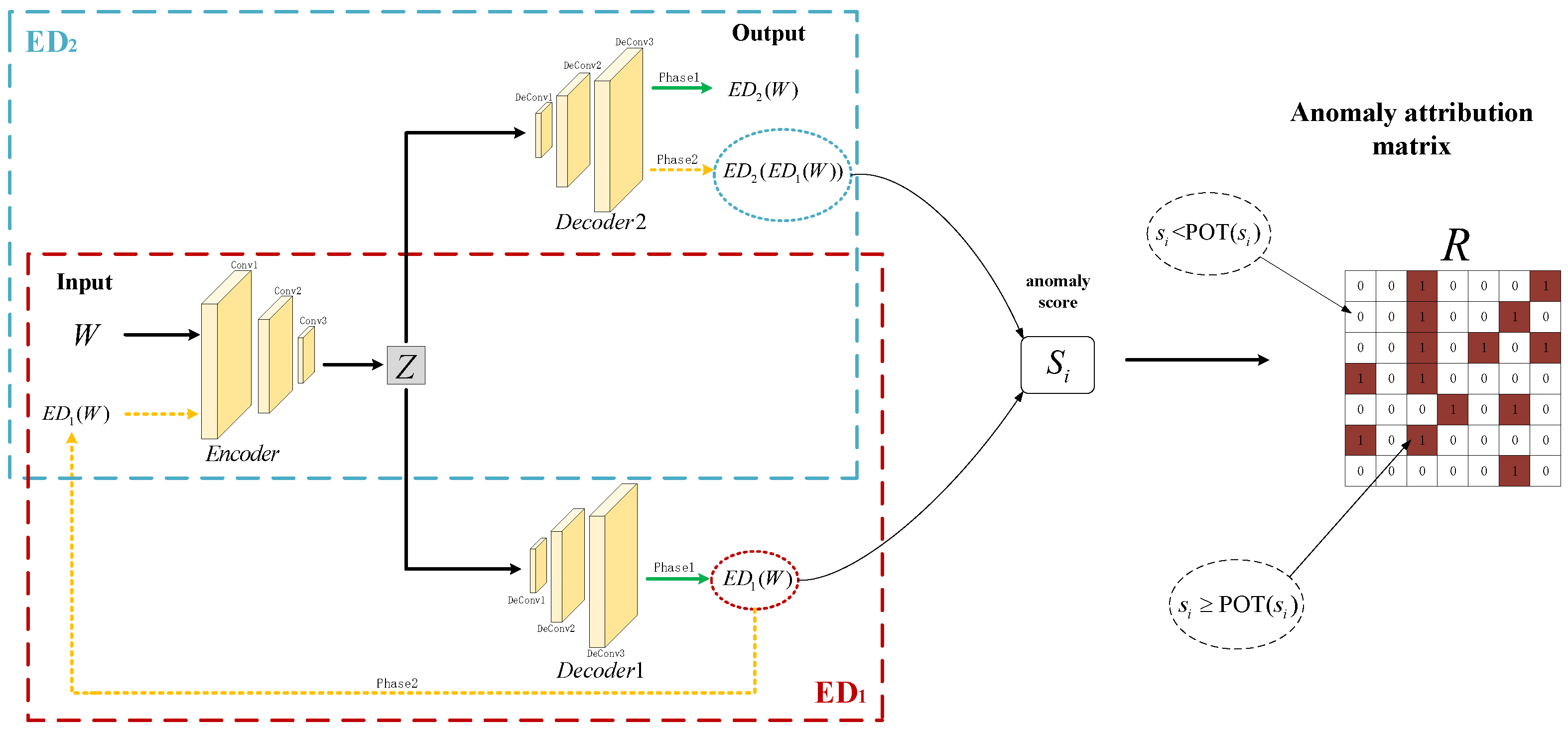
This section will describe the experimental environment, the datasets used, and the evaluation metrics used to evaluate the models we present.

4.1. Experimental Setup

To validate the effectiveness of the proposed CAT-IADEF, we have set up 5 experiments as follows:

(1)

Model Performance Comparison. Observe the performance of our method compared to the baseline method. The experimental results can be found in the “Anomaly detection” part in Section 4.4.

(2)

Anomaly Explanation Results. Anomaly Explanation Results of CAT-IADEF. The experimental results can be found in the “Anomaly explanation” part in Section 4.4.

(3)

Validation of Anomaly Explanation Framework. Validate the framework on different models. The experimental results can be found in the “Anomaly explanation” part in Section 4.4.

(4)

Ablation Analysis. Observe the effect of model components on model performance. The experimental results are shown in Section 4.5.

(5)

Sensitivity Analysis of Parameters. Observe the effect of different parameters on model performance. The experimental results are shown in Section 4.6.

Experimental Environments: (1) CPU: Intel (R) Core (TM) i7-7500U CPU@2.70 GHz; (2) RAM: 8 GB; (3) Python version: 3.7.11; and (4) Pytorch version: 1.6.0.

We selected the following methods for performance comparison experiments: PCA [6] based on dimensionality reduction, LOF [9] based on density, COPOD [8] based on statistics and machine learning, and OCSVM [11] based on classification; these four are relatively classic methods. MAD_GAN [22], OmniAnomaly [25], USAD [4], and TranAD [28] are the latest deep learning methods with excellent performances.

4.2. Public Datasets

We chose to use four datasets, including the Singapore Safe Water Treatment dataset; all selected datasets are detailed below and in

Table 1. Dataset data characteristics.

Name	Number of Instances	Train Ratio (%)	Test Ratio (%)	Number of Features	Anomaly Proportion (%)
SMAP	562,800	24.0	76.0	25	13.13
MSL	132,046	44.2	55.8	55	10.72
SWaT	946,719	52.5	47.5	51	11.98
SKAB	46,806	20.1	79.9	8	35.40

. For each dataset used, we selected multiple data subsets on which we trained and evaluated the models in our experiments.

SMAP. Soil collected by satellite comprises remote sensing information data [34]. Satellite-derived active and passive level 3 soil moisture observations were integrated into a modified two-layer Palmer model.

MSL. Similar to SMAP datasets. It consists of data collected by the Mars Science Laboratory [34] rover.

SwaT. Safe Water Treatment Dataset. Real-world industrial water treatment plants collect during the production of filtered water. It contains data from 7 days of regular operation and 4 days of abnormal function [35].

SKAB. A dataset is involved in evaluating anomaly detection algorithms [36]. The benchmark currently includes over 30 datasets and Python modules for evaluating algorithms. Each dataset represents a multivariate time series collected from sensors installed on the testbed.

Table 1 shows how many instances are included in each dataset, the ratio of training to testing, the number of features in each dataset, and the proportion of anomalies. The four open datasets are commonly used in anomaly detection, whose training/testing partition varies from dataset to dataset, and the number of features and anomaly ratios also vary among different datasets. We validate the effectiveness and robustness of our approach using various datasets with different proportions of anomalies, different partitions of training/test divisions, and different feature numbers.

4.3. Evaluation Measurements

4.3.1. Anomaly Detection Evaluation Metrics

We use a common accuracy, precision, recall, and F1 scores to evaluate the model performance [37].

4.3.2. Anomaly Explanation Settings

Through an independent matrix calculation framework, we directly give the serial numbers of the two dimensions with the most anomalies so that the relevant personnel can focus on observing the given dimensions when collecting this type of multivariate time series. This also, to a certain extent, makes it easier for researchers to review the data.

4.4. Experimental Results

Anomaly detection. Deep learning methods are known to be generally superior to machine learning methods. Still, machine learning methods may be better on some specific datasets, so, to show the overall performance of CAT-IADEF, we compare it with four classical methods and four deep learning methods. In the comparison experiments, to ensure the fairness of the comparison, we add dynamic threshold adjustment to all methods, and each group of experiments is carried out 5 times to obtain the average value.

Table 2. Performance comparison of CAT-IADEF and other methods on the subsets of data used.

Methods	P1 (SMAP)				T4 (MSL)				SWaT
	Acc	Pre	Rec	F1	Acc	Pre	Rec	F1	Acc	Pre	Rec	F1
PCA	0.890	0.110	0.999	0.198	0.934	0.031	0.999	0.060	0.858	0.394	0.696	0.503
LOF	0.794	0.691	0.999	0.817	0.931	0.410	0.999	0.581	0.813	0.978	0.696	0.813
COPOD	0.794	0.319	0.999	0.484	0.936	0.108	0.999	0.195	0.894	0.503	0.731	0.596
OCSVM	0.791	0.366	0.999	0.536	0.934	0.108	0.999	0.195	0.844	0.214	0.862	0.343
MAD_GAN	0.980	0.870	0.999	0.919	0.954	0.401	0.999	0.571	0.956	0.952	0.696	0.803
OmniAnomaly	0.982	0.859	0.999	0.924	0.965	0.441	0.999	0.612	0.959	0.976	0.969	0.812
USAD	0.980	0.849	0.999	0.918	0.969	0.488	0.999	0.648	0.959	0.989	0.688	0.811
TranAD	0.980	0.857	0.999	0.918	0.906	0.246	0.999	0.395	0.960	0.997	0.688	0.814
CAT-IADEF	0.981	0.857	0.999	0.923	0.979	0.596	0.999	0.747	0.958	0.971	0.696	0.811
Methods	Valve1-4 (SKAB)				Valve1-14 (SKAB)				T1 (SMAP)
	Acc	Pre	Rec	F1	Acc	Pre	Rec	F1	Acc	Pre	Rec	F1
PCA	0.376	0.319	0.999	0.483	0.367	0.350	0.999	0.519	0.700	0.300	0.999	0.461
LOF	0.323	0.384	0.999	0.555	0.350	0.401	0.999	0.572	0.472	0.944	0.999	0.971
COPOD	0.401	0.319	0.999	0.483	0.432	0.350	0.999	0.519	0.603	0.730	0.999	0.844
OCSVM	0.385	0.341	0.999	0.509	0.388	0.357	0.999	0.526	0.639	0.702	0.999	0.825
MAD_GAN	0.725	0.544	0.999	0.702	0.823	0.679	0.999	0.804	0.970	0.909	0.999	0.953
OmniAnomaly	0.760	0.770	0.940	0.840	0.770	0.740	0.980	0.850	0.975	0.923	0.999	0.960
USAD	0.912	0.801	0.999	0.885	0.929	0.860	0.999	0.914	0.971	0.912	0.999	0.954
TranAD	0.898	0.766	0.999	0.865	0.955	0.893	0.999	0.942	0.963	0.891	0.999	0.942
CAT-IADEF	0.951	0.868	0.999	0.929	0.991	0.974	0.999	0.987	0.975	0.923	0.999	0.960
Methods	D15 (MSL)
	Acc	Pre	Rec	F1
PCA	0.754	0.297	0.999	0.457
LOF	0.594	0.686	0.999	0.814
COPOD	0.625	0.542	0.999	0.703
OCSVM	0.754	0.610	0.999	0.758
MAD_GAN	0.974	0.919	0.999	0.957
OmniAnomaly	0.979	0.933	0.999	0.965
USAD	0.979	0.933	0.999	0.966
TranAD	0.917	0.781	0.999	0.877
CAT-IADEF	0.996	0.987	0.999	0.993

shows the accuracy, precision, recall, and F1 scores of CAT-IADEF and the other compared models on seven datasets.

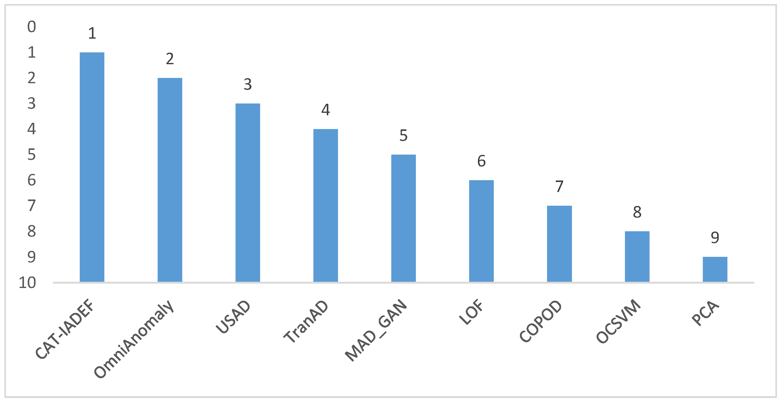
It can be seen from Table 2 that CAT-IADEF achieved the best F1 values on the data subsets T4 of MSL, Valve1-4 and Valve1-14 of SKAB, and D15 of MSL; these values were, respectively, 0.747, 0.929, 0.987, and 0.993. On the P1 subset of SMAP, OmniAnomaly’s method achieved the best F1 value of 0.924, and CAT-IADEF’s F1 value of 0.923 ranked second. On the data subset of SWaT, the TranAD method achieved the best F1 value of 0.814, and CAT-IADEF’s F1 value of 0.811 ranked fourth. On the data subset T1 of SMAP, the LOF method performed the best, with an F1 value of 0.971, and the F1 value of CAT-IADEF was 0.960, ranking second. We rank the F1 of the models comprehensively on all datasets, as shown in Figure 2. CAT-IADEF has a combined ranking of about 1.7, ranking first among all the compared models.

To analyze the different models, we first analyze four machine learning methods. The number of dimensionality reductions finally obtained by the PCA, that is, the number of latent variables, cannot be well estimated; therefore, its performance is not outstanding on the seven datasets. COPOD does not need to adjust parameters nor calculate the distance between samples, and the overhead is negligible. COPOD and OCSVM perform well on the T1 dataset and poorly on the rest of the datasets. This is due to the following problem: the scene changes in the face of non-stationary, unbalanced time series. The performance of LOF on other datasets is not outstanding. Still, the optimal F1 value is obtained on the T1 dataset, which is considered because this subset’s local distribution of the time series is suitable for calculating k-fields in LOF.

For the deep learning method, USAD only uses the simplest AE model and only considers the linear transformation, resulting in its insignificant effect, while CAT-IADEF adopts the CNN network and considers the relationship between different features. TranAD and MAN_GAN use an attention mechanism when detecting anomalies. TranAD uses positional encoding in the transformer structure to help capture the temporal order, which performs optimally on the SWaT dataset. OmniAnomaly is not the most prominent for all datasets except P1 because it is input sequentially, preserves essential information, and reconstructs all inputs regardless of input data, which prevents them from detecting anomalies that are close to normal trends. CAT-IADEF’s confrontational training allows it to magnify “slight” anomalies and help it see them, even though other models will detect “slight” anomalies as routine data.

Anomaly explanation. The results of the anomaly explanation are shown in

Table 3. Anomaly attribution of CAT-IADEF on different datasets.

P1 (SMAP)		T4 (MSL)		Valve1-4 (SKAB)
Dimension 1	Dimension 2	Dimension 1	Dimension 2	Dimension 1	Dimension 2
5	6	0	5	7	1
Valve1-14 (SKAB)		T1 (SMAP)		D15 (MSL)
Dimension 1	Dimension 2	Dimension 1	Dimension 2	Dimension 1	Dimension 2
7	1	0	5	0	5

, which we tested on the P1 dataset.

In Table 3, Dimension 1 is the dimension with the highest number of anomalies, and Dimension 2 is the dimension with the second highest number of anomalies. The number corresponding to the dimension is the serial number of the dimension. On the P1 dataset, for example, the dimension containing the most anomalies is Dimension 5, and the dimension with the second-most anomalies is Dimension 6.

To test the validity of the anomaly explanation, we tested five deep learning models, including CAT-IADEF, on experimental datasets.

Table 4. Validation of anomaly explanation.

Methods	P1 (SMAP)		T4 (MSL)		Valve1-4 (SKAB)
	Dimension 1	Dimension 2	Dimension 1	Dimension 2	Dimension 1	Dimension 2
MAD_GAN-EF	5	6	0	5	7	1
blackOmniAnomaly-EF	5	6	0	5	4	7
USAD-EF	5	6	0	5	1	7
TranAD-EF	0	3	0	5	1	7
CAT-IADEF	5	6	0	5	7	1
Methods	Valve1-14 (SKAB)		T1 (SMAP)		D15 (MSL)
	Dimension 1	Dimension 2	Dimension 1	Dimension 2	Dimension 1	Dimension 2
MAD_GAN-EF	7	4	0	5	0	5
blackOmniAnomaly-EF	4	7	0	5	0	5
USAD-EF	2	7	0	5	0	5
TranAD-EF	7	2	0	5	0	5
CAT-IADEF	7	1	0	5	0	5

shows that only TranAD attributes anomalies to Dimensions 0 and 3 on the dataset P1, and the remaining methods attribute anomalies to Dimensions 5 and 6. In the SKAB dataset, the percentage of anomalies is up to 35.4%. However, we can still see that the anomalies in the Valve1-4 dataset are mainly concentrated in Dimensions 7 and 1, and the Valve1-14 datasets are concentrated in Dimensions 7, 4, and 2. The results of the remaining datasets are similar and validate the validity of the anomaly explanation module.

4.5. Ablation Analysis

To investigate the importance of each model component to the overall model performance, we exclude each significant element in turn and observe how it affects model performance on the experimental dataset.

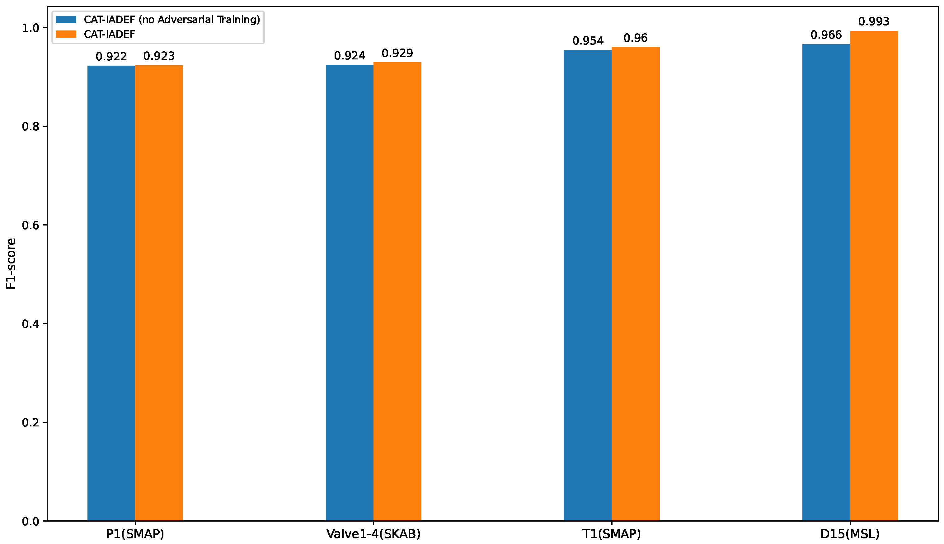
Adversarial training. In the experimental dataset, we compared the entire model to a model with no adversarial training, i.e., no $Decoder2$. Figure 3 shows the F1 scores of the CAT-IADEF and CAT-IADEF (no adversarial training) models on four experimental datasets.

As shown in Figure 3 the performance of CAT-IADEF (no adversarial) has declined on the four datasets, with a minimum drop of 0.11% and a maximum drop of 2.72%; this means that adversarial training enables the model to identify “slight” anomalies by magnifying errors.

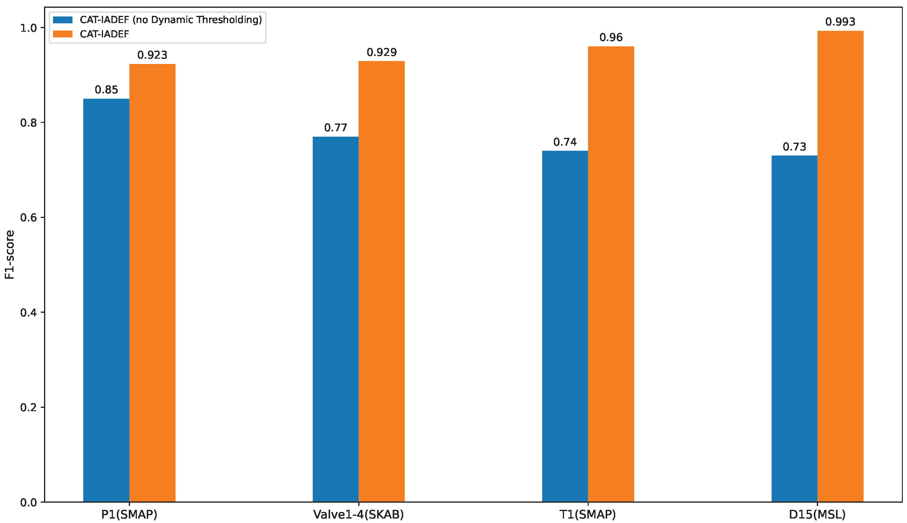
Dynamic threshold. We remove the dynamic threshold plate on CAT-IADEF and train it on the experimental dataset. Figure 4 shows the F1 scores of CAT-IADEF and CAT-IADEF (no dynamic threshold) on our four experimental datasets.

As shown in Figure 4, the POT dynamic selection threshold positively impacts the model. The most significant improvement is in the D15 dataset, from 0.73 to 0.993, representing 36.0% progress. The tiniest improvement is in the P1 dataset, from 0.85 to 0.923, representing an increase of 8.6%.

4.6. Sensitivity Analysis of Parameters

In the loss function, we have an $\alpha$ and $\beta$ to perform a weighted average of $Decoder1$ and $Decoder2$, $\alpha$ + $\beta$ = 1. When $\beta$ is 0 and $\alpha$ is 1, the loss function only considers the reconstruction loss from decoder1; when $\beta$ is 1 and $\alpha$ is 0, the model only considers the reconstruction loss of $Decoder2$ on the generated data. As shown in

Table 5. Performance comparison of different $\alpha$ and $\beta$ on P1 dataset.

$\mathit{\alpha }$	$\mathit{\beta }$	P	R	F1
0	1	0.8713	0.9999	0.9312
0.1	0.9	0.8730	0.9999	0.9322
0.3	0.7	0.8696	0.9999	0.9302
0.5	0.5	0.8478	0.9999	0.9176
0.7	0.3	0.8494	0.9999	0.9186
0.9	0.1	0.8494	0.9999	0.9186
1	0	0.8462	0.9999	0.9167

, we conducted experiments on the P1 dataset and considered 7 cases to illustrate the parameter pair impact on model performance.

It can be seen from Table 5 that when $\alpha$ + $\beta$ is changed from 0 to 1, the closer $\alpha$ is to 1 and the closer $\beta$ is to 0 (i.e., more consideration of the accurate data), the value of F1 tends to decrease, and F1 takes the maximum value. When $\alpha$ is closer to 0, $\beta$ is closer to 1 (i.e., more concerned with the reconstruction loss of the generated data, that is, the anomalies tend to the standard data in the simulated data). In reality, the training data is not necessarily normal, and the sensitivity study of $\alpha$ and $\beta$ can make the model more adaptable to different experimental environments.

5. Conclusions

We propose an anomaly explanation model based on adversarial convolution, which can perform anomaly detection and anomaly explanation on time series data of the cloud platform. Compared with the traditional linear change, its convolutional structure can share parameters, thereby significantly reducing the number of network parameters, which can effectively avoid overfitting. The adversarial-based training process enables the model to amplify “slight” anomalies, enhancing the model’s ability to identify anomalies that tend to be normal data. At the same time, the sensitivity setting of the adversarial training also makes the model applicable to a broader range of environments. Furthermore, POT optimizes detection intensively by modeling the tail of all values above a threshold. We also use loss function calculation for a simple attribution in the anomaly explanation part. We use seven data subsets of four public datasets to evaluate the model. The effect of the model also proves the effectiveness of the model type. Specifically, CAT-IADEF ranks first among all compared models, making CAT-IADEF a good choice for cloud platform anomaly detection.

In the future, we will consider adding an attention mechanism, such as a multi-head attention mechanism, to the overall model to allow the model to focus on some additional weird sequence points. We also want to be able to add residual connections to the convolutional network to speed up the model. Finally, we consider studying the cost and environmental analysis in the actual deployment process of the model and try to make it achieve low energy consumption and pollution.