Article

Spatial Evaluation of Machine Learning-Based Species Distribution Models for Prediction of Invasive Ant Species Distribution

1
Department of Biosystems Machinery Engineering, Chungnam National University, Daejeon 34134, Korea
2
Department of Smart Agriculture Systems, Chungnam National University, Daejeon 34134, Korea
*
Author to whom correspondence should be addressed.
These authors contributed equally to this work.
Appl. Sci. 2022, 12(20), 10260; https://doi.org/10.3390/app122010260
Submission received: 20 September 2022 / Revised: 5 October 2022 / Accepted: 8 October 2022 / Published: 12 October 2022

Abstract

:

Featured Application

This study offers fundamental insight for developing a model platform of artificial intelligence applicable for species distribution modeling, which has been currently emphasized for effective monitoring and control of invasive species.

Abstract

Recent advances in species distribution models (SDMs) associated with artificial intelligence (AI) and increased volumes of available data for model variables have allowed reliable evaluation of the potential distribution of any species. A reliable SDM requires suitable occurrence records and variables with optimal model structures. In this study, we developed three different machine learning-based SDMs [MaxEnt, random forest (RF), and multi-layer perceptron (MLP)] to predict the global potential distribution of two invasive ants under current and future climates. These SDMs showed that the potential distribution of Solenopsis invicta would be expanded by climatic change, whereas it would not significantly change for Anoplolepis gracilipes. The models were compared using model performance metrics, and the optimal model structure and spatial projection were selected. The MaxEnt exhibited high performance, while the MLP model exhibited low performance, with the largest variation by climate change. Random forest showed the smallest potential distribution area, but it was robust considering the number of occurrence records and changes in model variables. All the models showed reliable performance, but the difference in performance and projection size suggested that optimal model selection based on data availability, model variables, study objectives, or an ensemble approach was necessary to develop a comprehensive SDM to minimize modeling uncertainty. We expect that this study will help with the use of AI-based SDMs for the evaluation and risk assessment of invasive ant species.

1. Introduction

Global and local environmental variability has led to changes in the behavior and distribution of invasive pests and has necessitated early intervention, monitoring, and pest control. Species distribution models (SDMs) are a widely used tool for evaluating the potential distribution of a species; they utilize advanced artificial intelligence based on a machine learning algorithm for determining the environmental characteristics of potential habitats [1]. MaxEnt is a classical SDM in ecological niche modeling that employs maximum entropy theory to evaluate the probability of occurrence of a species as a function of model variables that code environmental characteristics [2]. Random forest (RF), a machine learning-based classifier, is another popular tool with a high classification performance used in computational ecology for identifying areas for the survival of target species [3]. Meanwhile, deep learning implemented with neural networks structured by a multi-layer perceptron (MLP) is the most recent approach that attempts to classify the potential or predicted presence and absence of a species. The application of MLP is relatively limited because of the challenges in determining the model structure and insufficient data to perform deep learning [4]. Nevertheless, advances in computing large data volumes and global concerns about invasive pests are accelerating the use of machine learning-based SDMs [5]. Therefore, there is an ongoing need for research to improve the performance of these models and optimize the selection of suitable models based on the target species, model variables, and data availability [6].
Ants are an intelligent species with high environmental adaptability and dispersion speed based on sociality through swarming; some invasive species have caused severe ecosystem damage [7]. Solenopsis invicta (Hymenoptera: Formicidae) and Anoplolepis gracilipes (Hymenoptera: Formicidae) are the most aggressive invasive ant species, and a global conservation campaign is underway to track and manage their invasions [8,9]. Solenopsis invicta, originating from South America and widely distributed throughout the US, has migrated to Asia and Australia [9,10,11]. Anoplolepis gracilipes is a tropical species that mostly inhabits southern Asia and a few areas in Central America and Oceania [8,10]. Their habitats are likely to expand; therefore, they have been selected as the target species for SDM because of the severe damage induced by them in the invaded regions [12,13,14,15,16,17].
Recently, enhancing the performance of an SDM has been issued, emphasizing high-quality data for model variables, advanced spatial processing, and a model using multiple machine learning algorithms. While there are a few sources to secure datasets for model variables, and spatial analysis tools for processing them, studies comparing machine learning-based models at the same time are limited. The high invasive risk of these ant species suggests a need to compare the model performance of the different types of machine learning-based SDMs to select the most appropriate model to identify the potential colonization areas of the ant species. The SDM characteristics can be analyzed in terms of data availability, model structures, and performance. In this study, three different machine learning-based models, including MaxEnt, RF, and MLP, were used to predict the spatial distribution of two invasive ant species, S. invicta and A. gracilipes, based on climate change. Thereafter, global projections from the three different models were compared in terms of area size, mean probability of occurrence, and optimal model structure.

2. Materials and Methods

2.1. Data Acquisition and Spatial Processing

The regions of occurrence of these species were obtained from the Centre for Agriculture and Bioscience International (CABI) and Global Biodiversity Information Facility (GBIF) public databases [18,19,20,21] and from the reports of previous studies [8,9]. The obtained records were cross-checked to minimize the uncertainty by screening for unreliable records, resulting in 6163 and 1297 points for S. invicta and A. gracilipes, respectively. Spatial filtering with a 20 km buffer was performed to adjust the uneven sampling points, which was essential to minimize the effect of sampling bias [22]. Thereafter, the coordinates that could not be georeferenced were removed. We confirmed the final georeferenced locations of 953 and 374 for S. invicta and A. gracilipes, respectively (Figure 1).

2.2. Climate Data

Historical (1970–2000) and future climate (2050) data coded by bioclimatic variables with a 10-min resolution were obtained from “www.worldclim.org (accessed on 13 July 2021)” to evaluate the current and future possibilities of the ant species occurring at these locations [23]. Future climate data was projected from the Shared Socio-economic Pathway (SSP) 585 and processed by the MIROC6 global climate model, which assumes rapid changes to simulate extreme cases for predictions [24,25].

2.3. Bioclimatic Variable Selection

The biological and ecological characteristics of the ant species were investigated to provide model variables, and correlations among bioclimatic variables at occurrence coordinates were identified to select model variables without model overfitting caused by multicollinearity [26]. Initially, bioclimatic variables were extracted at the sampling coordinates, and outliers that showed abnormal principal component scores in the principal component analysis of the extracted bioclimatic variables were filtered. To screen model variables, a correlation was examined for the whole set of variables, i.e., bioclimatic variables and elevation, with the threshold value of the correlation coefficient 0.7 to the reference variable that was biologically driven.
For S. invicta, we first investigated the biological and ecological characteristics to relate them to the selection of model variables. Relatively high temperatures and precipitation were defined as characteristic environmental conditions based on the general habitat distribution in tropical and subtropical regions. Low temperatures and low precipitation may limit the occurrence of S. invicta, suggesting that climatic characteristics are suitable candidates for model variables. Moreover, Byeon et al. [27] reported that low temperature and soil moisture limited population growth and development, as well as foraging activity, which supports the confining effect of climatic conditions on the habitat of S. invicta. We derived bio- 1, 5, 6, 10, and 11, which were the variables coded with annual, high, and low temperatures, and bio- 12, 13, 14, 16, and 17, which were related to annual, high, and low precipitation conditions. We then statistically investigated the variations in the coefficient for each bioclimatic variable because its low variation could indicate the most suitable climatic characteristics for the habitat depending on the species’ biology and ecology. It was relatively small in bio- 1, 5, and 10, which suggests its robustness and confirms the effect of climatic conditions on limiting or accelerating habitat expansion. For precipitation, bio12 showed the lowest coefficient of variation; thus, it was selected as a model variable. We removed variables that were correlated with the biologically driven variables larger than 0.7; bio- 4, 6, 7, and 11—which were correlated with bio1—were removed, while bio- 2, 3, 8, and 9 were included as their correlation values were less than the selected threshold. Moreover, because of the high correlation between bio- 5 and 10, only bio5 was retained because extreme temperatures limit the biological activity of S. invicta [28]. Bio- 12, 13, 16, 17, 18, and 19 were removed, while bio- 14 and 15 were included because of their low correlation with the other variables. Therefore, we determined nine bioclimatic variables in addition to elevation (Table 1).
A similar procedure was performed for A. gracilipes; however, the available research is relatively limited compared with that for S. invicta. Therefore, bioclimatic variables were screened by considering the climatic properties of the geographic areas [29]. The initial bioclimatic variables for S. invicta were used as the starting point because A. gracilipes mainly inhabits tropical regions; this resulted in the selection of bio- 1, 5, 6, 10, 11, 12, 13, 14, 16, and 17. Due to the low coefficient variations, we first selected bio- 1 and 5. Subsequently, bio- 6, 8, 9, 10, and 11 were removed because of their high correlation (r > 0.7), and bio- 2 and 7 were included because they were not correlated with the other variables. Bio- 3 and 4 were correlated with each other; however, bio3 was selected because its correlation coefficients with other variables were lower than those of bio4. For precipitation, a previous study showed that seasonality was evident for nests, which mainly occurred during the wet season [30]. For this reason, we selected bio- 15 and 16, representing the seasonality of the precipitation and the precipitation during the wettest quarter, respectively. Due to their high correlations with bio- 15, and 16, bio- 12, 13, 14, and 17 were removed. Bio- 18 and 19 were included as they were not correlated with the other bioclimatic variables. Finally, nine bioclimatic variables and elevations were selected for use in the models (Table 1).

2.4. MaxEnt Operation

MaxEnt is an algorithm in species distribution modeling that estimates the occurrence probability of a target species based on the maximum entropy theory (Phillips and Dudík, 2008). MaxEnt requires optimal conditions for model features and regularization multiplier, which are related to structural complexity [31]. In this study, MaxEnt was operated with optimal features and a regularization multiplier determined by ENMeval [31]. For both ant species, the optimal model features were linear, quadratic, product, threshold, and hinge features, while the regularization multipliers were 0.5 and 1.0 for S. invicta and A. gracilipes, respectively. We used 10-fold cross-validation to run the model with 10,000 random background points and did not use a biased background because spatial filtering had already been performed for sufficient occurrence records [32]. The output was stored in an ASCII file in a logistic-type format, which presented the possibility of occurrence under the given bioclimatic conditions. Then, potential distribution regions were built in binary and gradient format, which were finally saved in the form of an shp file to present it as an image. Model performance was evaluated by calculating true skill statistics (TSS) using R software [33] in addition to areas under the receiver operating characteristic (ROC) curve (AUC) because TSS is a more practical and realistic measure of the performance of machine learning-based SDMs [34]. In addition, we also calculated partial AUC (pAUC) by considering the region of ROC space having less omission error than the variable [35]. In general, AUC larger than 0.8 or TSS larger than 0.6 indicates a good model performance, while pAUC larger than 1 indicates a good model performance. The average threshold values for the 10-fold calculation of TSS were 0.142 and 0.196 for S. invicta and A. gracilipes, respectively, which maximized the sum of sensitivity and specificity [36]. The output of occurrence possibility was projected as a binary map with a threshold value criterion determined for TSS using ArcMap version10.4.1 (ESRI, Redlands, CA, USA).

2.5. Random Forest Operation

Random forest is a machine learning algorithm that develops many classification trees for bootstrap samples randomly selected from the original data [37]. In this study, we used RF in the R package to classify the presence and absence of the two ant species [38]. The dataset for RF was developed by integrating the geographic records and background data that were randomly selected on the world map to have a 50:50 split of presence and absence data for each ant species. The dataset was separated into 80% for model training and 20% for testing the RF model. The number of variables in the random subset at each node (mtry) was determined by the square root of the number of variables [39], resulting in 3 out of 10 selected bioclimatic variables for each ant species. Another parameter, the number of trees (ntree, the number of bootstrap samples), was estimated to be 500, which showed the lowest out-of-bag estimate of error rate (OOB error) under fixed mtry of 3 for both ant species. The confusion matrix was calculated to evaluate TSS as a model performance metric in addition to AUC, and variable importance was assessed using mean decrease accuracy (MDA), which estimates the increase in OBB error by generating permutations of one variable while maintaining constant values for other values [38]. The classification result was georeferenced and projected onto a world map using ArcMap.

2.6. Artificial Neural Network Construction

Artificial neural networks (ANN) are basic deep-learning algorithms that imitate the functionality of human brains by interconnected layers and neurons and have been used to predict the potential presence of insect species [40]. This study employed MLP models with the same model variables and presence data used for MaxEnt and RF using Keras in Python [41,42]. Among occurrence records and background points, 20% of them were used to test the model, while 80% was further split into 80% for training and 20% for validating the model. We developed a simple MLP structure because of the relatively small amount of data in deep learning. To determine the optimal model structure, the number of neurons was varied from 4 to 30, with 10 running trials for each number of neurons. The batch size was determined to be equal to the number of training data, whereas the epoch and learning rate were set to show a stable loss function and accuracy [43]. The loss function was observed for each model to avoid under or overfitting. In addition to the loss function, the average TSS values for 10 trials in each model structure were calculated by selecting the threshold value that resulted in the highest TSS [36]. The optimal model structure was determined based on the loss function and the average TSS value. Thereafter, a three-layer MLP model composed of two hidden layers was employed, in addition to an output layer of two neurons representing the presence and absence probabilities. The number of hidden layers was 11-11 and 9-9 for S. invicta and A. gracilipes, respectively, which were applied to predict the occurrence possibility of the two ant species at global georeferenced points, and were finally projected onto the world map using ArcMap.

3. Results

3.1. Performance Comparison by Models

All model performances exceeded 0.8, except for TSS values of 0.783 in the MLP model of A. gracilipes, suggesting that the developed model is reliable for predicting the potential distribution of the two ant species (Table 2). In particular, the AUC exceeded 0.89 for all models in both species with high accuracy and sensitivity, which indicated an accurate assessment of the actual occurrence.
In terms of model type, the MaxEnt model exhibited the highest performance, whereas the MLP model showed the lowest value for both species, possibly due to low specificity. When comparing the performance metrics, the AUC showed a relatively higher value than the TSS values, regardless of model and species. The MLP model showed the largest difference between the AUC and TSS, suggesting its relatively high dependency on the sampling size compared to others. All the models showed pAUC larger than 1, consistent with other metrics showing a good model performance. In this metric, the MLP showed the lowest value, while the MaxEnt and RF showed similarly high values. When considering the number of occurrence data that differed by species in the same model, the AUC of the MaxEnt model for A. gracilipes was larger than that for S. invicta, whereas MLP exhibited a higher AUC in the S. invicta model than in A. gracilipes. Thus, AUC may be affected by the type of model rather than the sample size, whereas the MPL model had a relatively high dependency on the sample size. Both MaxEnt and MLP models exhibited higher TSS in the S. invicta model than in the A. gracilipes, suggesting that TSS was more sensitive to sample size compared with AUC and pAUC. Random forest exhibited consistent values for AUC and TSS for each species; thus, the difference between AUC and TSS was almost constant. A similar consistency was also shown in the pAUC and accuracy, indicating relatively higher robustness for the sample size of the RF model compared with other models.
Overall, MaxEnt showed the best performance for both species, whereas RF resulted in consistent results even with a small sample size. In addition, larger datasets for MLP model training may lead to improved model performance, but at present, lower performance compared to the other models was demonstrated.

3.2. Spatial Projection Comparison by Models

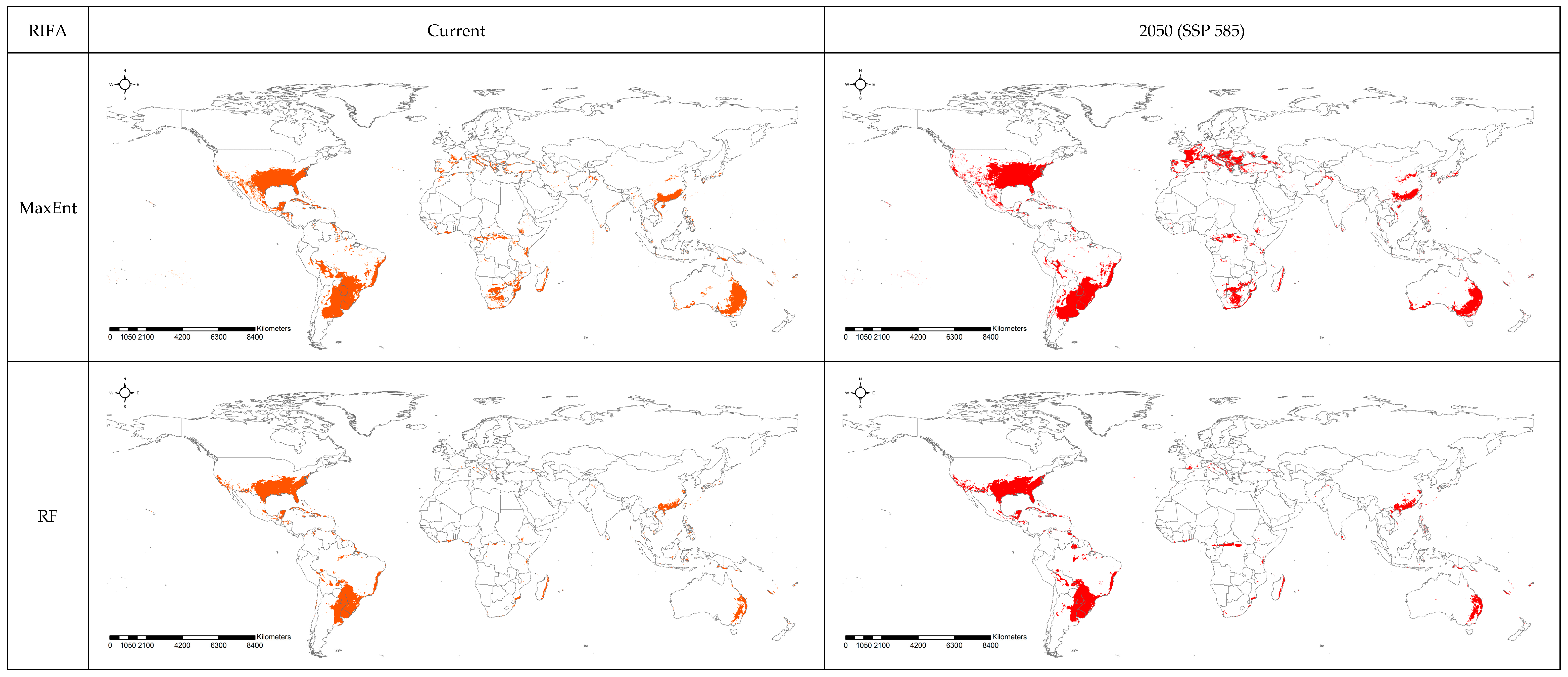
The overall global potential distributions of the two ant species were predicted using the occurrence data. Solenopsis invicta was predicted to be densely distributed in North and South America, where most of the occurrence data were concentrated, and showed some potential presence in Africa, Asia, and Australia (Figure 2). Europe was predicted to be an at-risk area for S. invicta distribution in MaxEnt and MLP models, whereas RF expected only a rare chance of its occurrence under the current climate conditions in Europe. The potential distribution areas—the ratio of predicted occurrence area to the whole world calculated by counting the cell numbers in the map—of S. invicta under the current climate for the MaxEnt, RF, and MLP models were estimated to be 5.2%, 4.0%, and 6.5%, respectively (Table 3). When applying the climate change scenario, all the models predicted that the potential occurrence area of S. invicta would expand. The MaxEnt, RF, and MLP models predicted 5.6%, 4.3%, and 16.5% of the ratio of potential occurrence area to the whole world, respectively, and high variation was observed in the MLP model compared to the MaxEnt and RF models. In addition, European regions were vulnerable to significant S. invicta invasions.
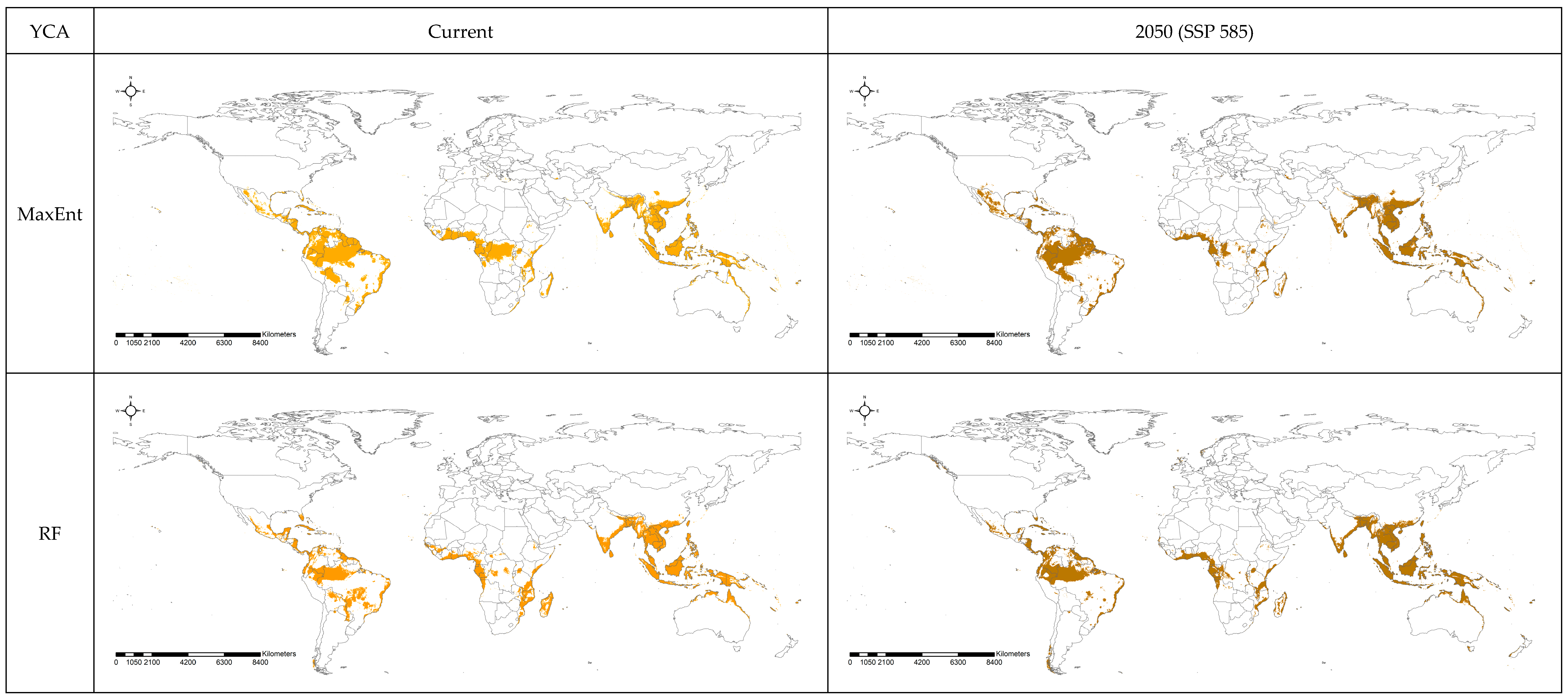
Similarly, the potential distribution of A. gracilipes was mainly predicted in Southeast Asia, in addition to Central America (Figure 3). Notably, large areas in South America were predicted to be at risk of A. gracilipes, although there was no current occurrence data. For A. gracilipes, the ratios of potential distribution areas to the whole world were 7.3%, 8.4%, and 21.8%, estimated by MaxEnt, RF, and MLP models, respectively, revealing significantly larger projections in the MLP model. In contrast to S. invicta, it was predicted that areas of A. gracilipes’ potential distribution would not be significantly affected by climate change but rather would be reduced slightly without further habitat expansion. Quantitatively, the potential areas predicted by MaxEnt, RF, and MLP models were 6.1%, 7.8%, and 17.8%, respectively, reducing by 0.5–4% for each model. In general, the MLP model produced the largest area of potential distribution for both species and the highest variations due to climate change, whereas RF exhibited the lowest variations in potential distribution (<1%) for both species due to climate change.
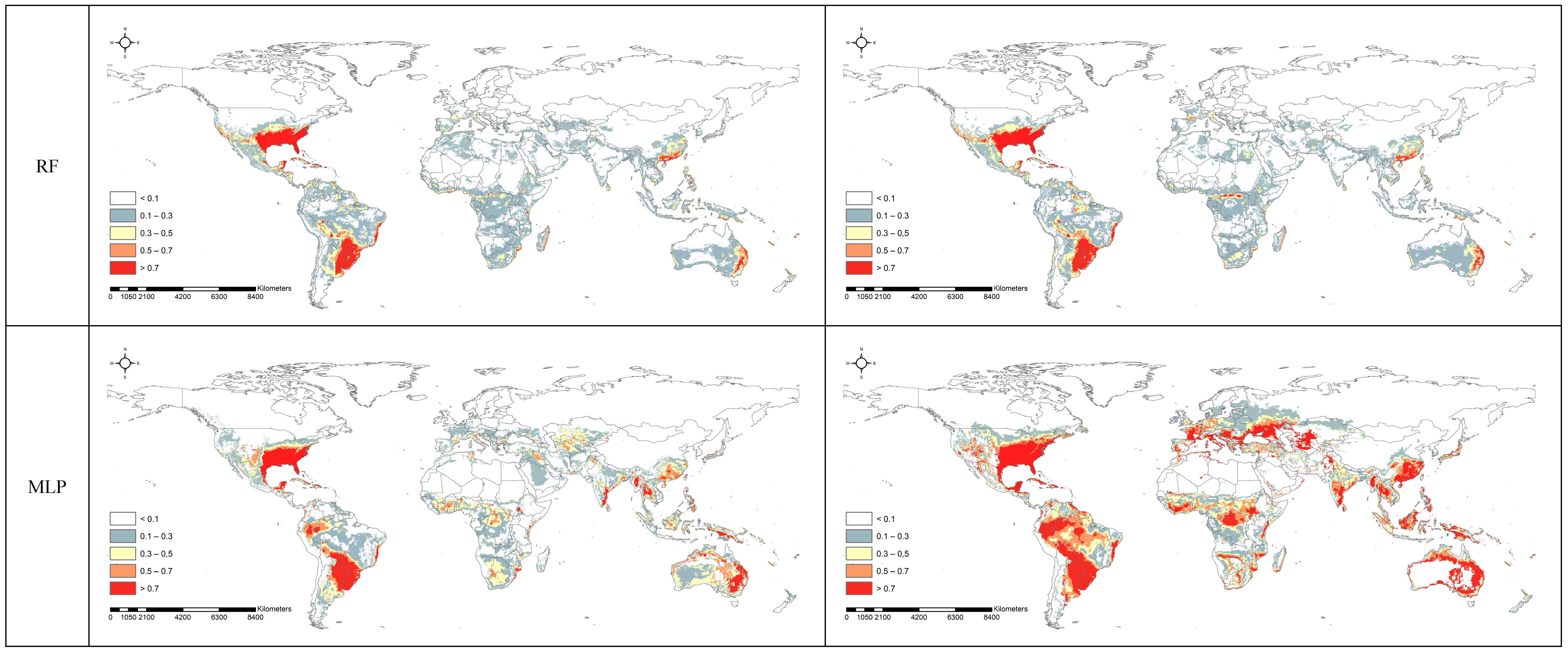
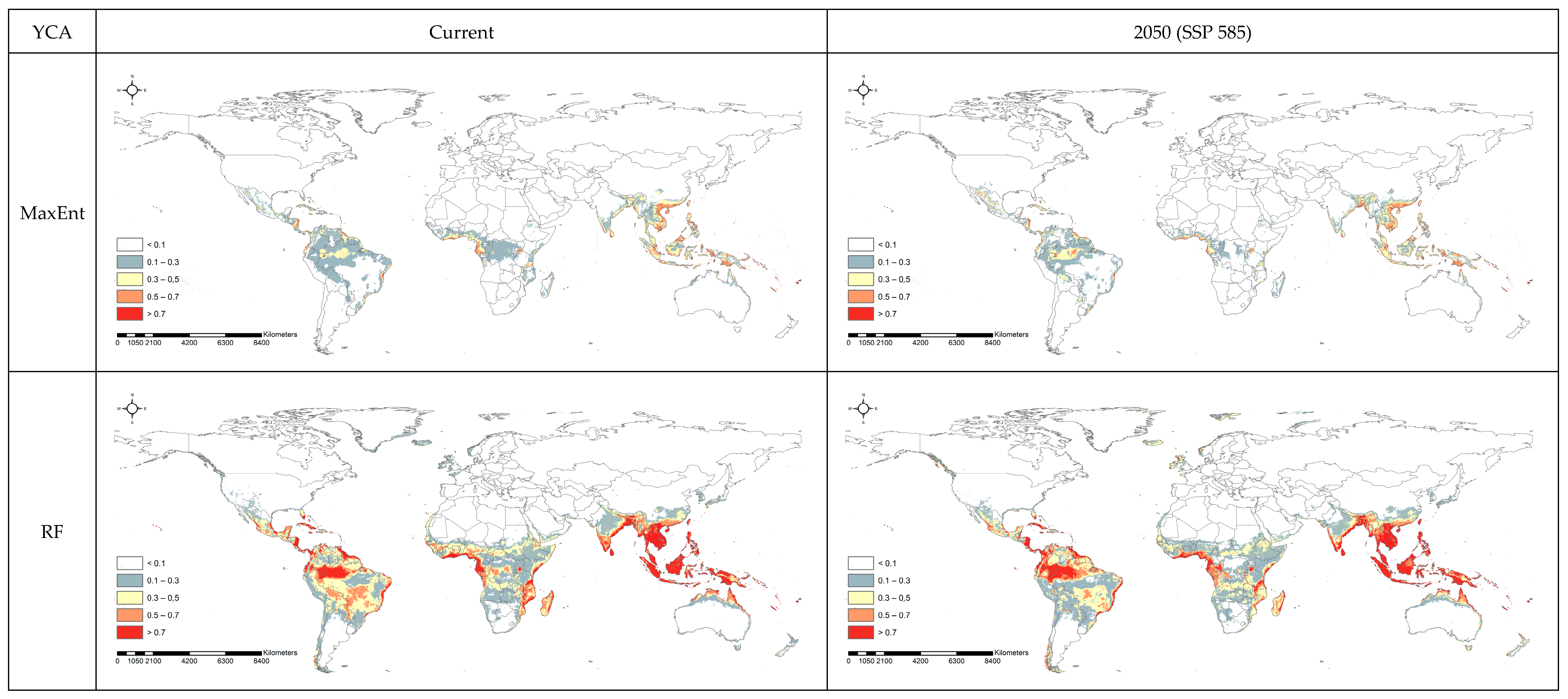
The average probability projected by regression differed according to the model, showing similar results for RF and MLP in contrast to MaxEnt (Figure 4 and Figure 5). The average current possibility predicted by MaxEnt was the lowest, at 0.307 and 0.317 for S. invicta and A. gracilipes, respectively. The highest average probability was predicted by RF for S. invicta, whereas MLP showed the highest possibility for A. gracilipes under the current climate. It is expected that the occurrence possibility of S. invicta will remain relatively unchanged in 2050, with the largest variation in the RF model (1.5%). In contrast, relatively large variations in the occurrence possibility of A. gracilipes were predicted in 2050 compared to the current climate, showing 2–4% variations depending on the model used. In general, MLP predicted a relatively higher occurrence probability, whereas MaxEnt predicted the lowest worldwide occurrence probability, regardless of species and climate change.

4. Discussion

In this study, three different SDMs were developed to implement machine learning algorithms. The AUC exhibited a value near or above 0.9, regardless of the model, which suggests excellent performance of the developed models [44]. Compared to AUC, a relatively lower TSS value was obtained for all models, with the highest result in the MaxEnt model. In contrast, the MLP model showed lower TSS compared to the other models, which is consistent with a previous modeling study for S. invicta and may be due to the amount of data used for model training [15]. This could be observed in the MLP models for both ant species, as ~2.5 times more data were used to develop the model for S. invicta than for A. gracilipes. In addition, the relatively small amount of data used in the A. gracilipes MLP model exhibited significantly less specificity compared to the sensitivity in the same model, as well as compared to other models. This suggests that insufficient data points may be a source of uncertainty [45,46]. Compared to the MLP model, the RF algorithm showed only a 0.3% and 0.1% difference in the TSS and accuracy, respectively, between S. invicta and A. gracilipes, suggesting robustness even with small sample sizes [15,47]. This advantage of RF in SDM is consistent with similar performance and spatial projection of S. invicta in a previous study, where a boosted regression tree was used [17]. Finally, there still exists controversy on model performance metrics due to dependency on prevalence, suggesting the necessity of using multiple metrics to confirm the model performance [48,49,50].
MaxEnt and RF had similar spatial projection sizes. MaxEnt is a specialized SDM tool [2]; thus, it has an algorithm suitable for data generally used in SDM. The RF algorithm has also been used for ecological modeling to define areas of species occurrence because it can overcome limited data points [46,51]. However, the MLP model predicted larger presence areas than MaxEnt and RF, suggesting the necessity of sufficient data to train deep learning models [52]. This can be shown by the areal sizes of S. invicta and A. gracilipes predicted by the MLP model. For S. invicta, which used 2.5 times more coordinates than A. gracilipes, the MLP model projection under the current climate was ~1–2% larger than those by MaxEnt and RF. For A. gracilipes, the MLP model projection was 14–15% times larger compared to the other models. This suggests that more data points might be necessary to develop an MLP model that is comparable with MaxEnt and RF. Areal variation due to climate change was the least in RF, suggesting that RF was relatively insensitive to model variables, which is consistent with the observation of a previous study showing the least projection areas of S. invicta by RF [15,53]. In contrast, the MLP model produced the largest variation in projection areas for both species due to climate change, showing a sensitive response to changes in model variables that might be due to a dependency on initial model variable weight [54]. Therefore, a developed MLP model can be an option to record changes in species distribution due to climate change, but cautious interpretation is necessary when considering other comparable models.
The CLIMEX model is a mechanistic SDM tool for evaluating the habitats of a species that is climatically suitable for species biology [12,14]. This model predicted areas for both species that were much larger than those of this study because CLIMEX finds an area where species biology can endure a regional climate [55]. Only MLP showed areal projections similar to the CLIMEX results for A. gracilipes, but this might be due to the limited training data. The current results were similar to the projections by the genetic algorithm for rule-set prediction (GARP) and BioClim [13]. This suggests that statistics-based models, including machine learning algorithms, commonly predict core habitats around occurrence coordinates, but the areal size can differ according to the specific model. Therefore, appropriate model selection for the purpose of a study is crucial, as is highlighting the current application of ensemble models to project occurrence areas conservatively by extracting consensus areas from each model [27]. In contrast to the areal size by classification, the occurrence possibility by regression was similar between RF and MLP, and they were ~2.5 times higher than the occurrence possibility evaluated by MaxEnt. MaxEnt uses the maximum entropy model to calculate the occurrence possibility [2], whereas RF and MLP are universal classifiers that calculate probability based on the weight of model variables [3,4]. Different thresholds for classification are necessary for each model to project similar distribution patterns. Recently, a value that maximizes the TSS has been proposed as the threshold value, which is the value used in this study [34]. In addition, MaxEnt requires the determination of optimal model features, and delta Akaike Information Criterion (AIC) has been mostly used for selecting the best model settings. However, threshold-dependent evaluation metrics could be a better option because AIC-based selection can result in low predictive performance due to oversimplification of the model [56]. This suggests the necessity of defining the best model in ecological niche modeling when using the MaxEnt. Therefore, we believe that either classification works better with the simultaneous use of different machine learning-based models than a regression method to evaluate a specific probability. A specific method that can adjust different occurrence probabilities needs to be considered to calculate the occurrence probability [57].
Although the MLP model exhibited the lowest model performance owing to the small number of data points available for model training, its performance for both species was reliable, suggesting its potential for SDM applications [4,58]. When developing an MLP model, one of the most challenging tasks is to determine the hyperparameters necessary for determining the optimal model structure related to the number of hidden layers and neurons. This process mostly depends on the intuition of the researcher based on variations in the loss function; thus, a formalized method that is applicable to SDM is necessary [58]. In this study, the model performance metrics evaluated by the test dataset were used to determine the optimal model structure. All model metrics, including TSS and accuracy, were almost saturated as the number of neurons increased, indicating that there was a minimum threshold value that guaranteed model performance. Therefore, we believe that TSS can be used as an index to objectively determine the structure of the MLP model in the SDM, in addition to the loss function.
One of the main purposes of SDM is to derive ecological insights into species distributions. This is generally conducted by analyzing the contribution or importance of model variables, which reflect the environmental characteristics of species’ habitat and biology. Variable contribution and mean decrease in accuracy are widely used measures of variable importance in MaxEnt and RF, respectively. In both models, the important variables showed similar trends for both the ant species. Bio1 (annual mean temperature) and bio14 (precipitation seasonality) were the two most important variables suggested by both MaxEnt and RF for S. invicta, which is consistent with a previous study that reported bio14 to be the most important variable in RF because variations in soil humidity related to precipitation seasonality affect the survival of S. invicta [15,59]. In addition, low and extremely high temperatures are unfavorable for S. invicta [16,60], justifying the importance of monitoring annual average temperature in predicting S. invicta occurrence areas. For A. gracilipes, bio7 (annual temperature range) was the most important variable in MaxEnt, whereas it was the second most important variable in RF after bio2 (mean diurnal range). Anoplolepis gracilipes is distributed year-round in tropical areas with high temperatures near the equator [8]; thus, its habitat can be confined by temperature range, represented by bio- 7 and 2. Bio16 (the precipitation of the wettest quarter) showed the second highest contribution in MaxEnt, while it was fifth in order in MDA in RF by a small margin, consistent with its preference for wet regions, even though it could adapt to very low precipitation [61,62]. For both models, elevation was not a significant variable, suggesting that the aggressive mobility of the two invasive ant species can survive at any altitude as long as the environment is suitable [8,17]. In contrast to MaxEnt and RF, it is difficult to measure variable importance in the MLP model, as weights among neurons are inside the black box. For this reason, the MLP model is better for use in conjunction with other machine learning algorithms in SDM, which analyzes the ecological aspects from the modeling results.

5. Conclusions

Owing to the large emphasis on artificial intelligence, machine learning algorithms have been actively applied to ecological niche modeling. This study compared the model performance and spatial projection of three different SDMs, which employed a machine learning-based algorithm to evaluate the potential distribution of two invasive ant species. Our findings revealed a crucial point in the selection of machine learning-based SDM. The model performance differed according to the type of model and the amount of available data. Hence, the model needs to be selected based on data availability along with the study purpose, including the target species, areal size, and model variables. Moreover, an ensemble model that simultaneously uses more than one model can provide a conservative evaluation by compensating for the discrepancy among models. In addition, a practical metric for evaluating the model performance should be considered to select an optimal model algorithm and its structure, as shown in the MLP model in this study. Even though this study used bioclimatic variables and elevation as model variables, one of the biggest advantages of the machine learning algorithm in SDM is the flexibility of variable addition, suggesting that a model with high reliability can be developed with additional variables, such as soil temperature for ant species that live underground [63].

Author Contributions

Conceptualization, W.-H.L.; methodology, W.-H.L. and J.-W.S.; software, W.-H.L., J.-W.S., S.-H.Y. and J.-M.J.; validation, W.-H.L. and J.-W.S.; formal analysis, W.-H.L., J.-W.S. and S.-H.Y.; investigation, W.-H.L., J.-W.S., S.-H.Y. and J.-M.J.; resources, W.-H.L., J.-W.S., S.-H.Y. and J.-M.J.; data curation, W.-H.L. and J.-W.S.; writing—original draft preparation, W.-H.L. and J.-W.S.; writing—review and editing, W.-H.L., J.-W.S. and J.-M.J.; visualization, W.-H.L. and J.-W.S.; supervision, W.-H.L.; project administration, W.-H.L.; funding acquisition, W.-H.L. All authors have read and agreed to the published version of the manuscript.

Funding

This work was supported by Chungnam National University.

Institutional Review Board Statement

Not applicable.

Informed Consent Statement

Not applicable.

Data Availability Statement

The data presented in this study are available on request from the corresponding author.

Conflicts of Interest

The authors declare no conflict of interest.

References

  1. Gobeyn, S.; Mouton, A.M.; Cord, A.F.; Kaim, A.; Volk, M.; Goethals, P.L. Evolutionary algorithms for species distribution modelling: A review in the context of machine learning. Ecol. Model. 2019, 392, 179–195. [Google Scholar] [CrossRef]
  2. Phillips, S.J.; Dudík, M. Modeling of species distributions with Maxent: New extensions and a comprehensive evaluation. Ecography 2008, 31, 161–175. [Google Scholar] [CrossRef]
  3. Evans, J.S.; Murphy, M.A.; Holden, Z.A.; Cushman, S.A. Modeling Species Distribution and Change Using Random Forest; Springer: New York, NY, USA, 2011; pp. 139–159. [Google Scholar] [CrossRef]
  4. Muñoz-Mas, R.; Martínez-Capel, F.; Alcaraz-Hernández, J.D.; Mouton, A.M. On species distribution modelling, spatial scales and environmental flow assessment with Multi–Layer Perceptron Ensembles: A case study on the redfin barbel (Barbus haasi; Mertens, 1925). Limnologica 2017, 62, 161–172. [Google Scholar] [CrossRef]
  5. Li, X.; Wang, Y. Applying various algorithms for species distribution modelling. Integr. Zool. 2013, 8, 124–135. [Google Scholar] [CrossRef]
  6. Araújo, M.B.; Guisan, A. Five (or so) challenges for species distribution modelling. J. Biogeogr. 2006, 33, 1677–1688. [Google Scholar] [CrossRef]
  7. Siddiqui, J.A.; Bamisile, B.S.; Khan, M.M.; Islam, W.; Hafeez, M.; Bodlah, I.; Xu, Y. Impact of invasive ant species on native fauna across similar habitats under global environmental changes. Environ. Sci. Pollut. Res. 2021, 28, 54362–54382. [Google Scholar] [CrossRef] [PubMed]
  8. Wetterer, J.K. Worldwide distribution and potential spread of the long-legged ant, Anoplolepis gracilipes (Hymenoptera: Formicidae). Sociobiology 2005, 45, 77–97. [Google Scholar]
  9. Ascunce, M.S.; Yang, C.C.; Oakey, J.; Calcaterra, L.; Wu, W.J.; Shih, C.J.; Goudet, J.; Ross, K.G.; Shoemaker, D. Global invasion history of the fire ant Solenopsis invicta. Science 2011, 331, 1066–1068. [Google Scholar] [CrossRef]
  10. Holway, D.A.; Lach, L.; Suarez, A.V.; Tsutsui, N.D.; Case, T.J. The causes and consequences of ant invasions. Annu. Rev. Ecol. Syst. 2002, 33, 181–233. [Google Scholar] [CrossRef] [Green Version]
  11. Morrison, L.W.; Porter, S.D.; Daniels, E.; Korzukhin, M.D. Potential global range expansion of the invasive fire ant, Solenopsis invicta. Biol. Invasions 2004, 6, 183–191. [Google Scholar] [CrossRef]
  12. Sutherst, R.W.; Maywald, G. A climate model of the red imported fire ant, Solenopsis invicta Buren (Hymenoptera: Formicidae): Implications for invasion of new regions, particularly Oceania. Environ. Entomol. 2005, 34, 317–335. [Google Scholar] [CrossRef]
  13. Chen, Y. Global potential distribution of an invasive species, the yellow crazy ant (Anoplolepis gracilipes) under climate change. Integr. Zool. 2008, 3, 166–175. [Google Scholar] [CrossRef] [PubMed]
  14. Jung, J.M.; Byeon, D.H.; Jung, S.H.; Yu, Y.M.; Yasunaga-Aoki, C.; Lee, W.H. Global Prediction of Geographical Change of Yellow Crazy Ant (Anoplolepis gracilipes) Distribution in Response to Climate Change Scenario. J. Fac. Agric. Kyushu Univ. 2017, 62, 403–410. [Google Scholar] [CrossRef]
  15. Sung, S.; Kwon, Y.S.; Lee, D.K.; Cho, Y. Predicting the potential distribution of an invasive species, Solenopsis invicta Buren (Hymenoptera: Formicidae), under climate change using species distribution models. Entomol. Res. 2018, 48, 505–513. [Google Scholar] [CrossRef]
  16. Byeon, D.H.; Lee, J.H.; Lee, H.S.; Park, Y.; Jung, S.; Lee, W.H. Prediction of spatiotemporal invasive risk by the red imported fire ant (Hymenoptera: Formicidae) in South Korea. Agronomy 2020, 10, 875. [Google Scholar] [CrossRef]
  17. Chen, S.; Ding, F.; Hao, M.; Jiang, D. Mapping the potential global distribution of red imported fire ant (Solenopsis invicta Buren) based on a machine learning method. Sustainability 2020, 12, 10182. [Google Scholar] [CrossRef]
  18. CABI (Centre for Agriculture and Bioscience International). Available online: www.cabi.org/isc/datasheet/5575 (accessed on 30 June 2020).
  19. GBIF (Global Biodiversity Information Facility). Available online: https://doi.org/10.15468/dl.6zb5ah (accessed on 30 June 2020).
  20. CABI (Centre for Agriculture and Bioscience International). Available online: www.cabi.org/isc/datasheet/50569 (accessed on 28 June 2021).
  21. GBIF (Global Biodiversity Information Facility). Available online: https://doi.org/10.15468/dl.8q7ydm (accessed on 28 June 2021).
  22. Brown, J.L.; Anderson, B. SDMtoolbox: A python-based GIS toolkit for landscape genetic, biogeographic and species distribution model analyses. Methods Ecol. Evol. 2014, 5, 694–700. [Google Scholar] [CrossRef]
  23. Fick, S.E.; Hijmans, R.J. WorldClim 2: New 1-km spatial resolution climate surfaces for global land areas. Int. J. Climatol. 2017, 37, 4302–4315. [Google Scholar] [CrossRef]
  24. van Vuuren, D.P.; Carter, T.R. Climate and socio-economic scenarios for climate change research and assessment: Reconciling the new with the old. Clim. Chang. 2014, 122, 415–429. [Google Scholar] [CrossRef] [Green Version]
  25. Schandl, H.; Lu, Y.; Che, N.; Newth, D.; West, J.; Frank, S.; Obersteiner, M.; Rendall, A.; Hatfield-Dodds, S. Shared socio-economic pathways and their implications for global materials use. Resour. Conserv. Recycl. 2020, 160, 104866. [Google Scholar] [CrossRef]
  26. Yoon, S.; Lee, W.H. Methodological analysis of bioclimatic variable selection in species distribution modeling with application to agricultural pests (Metcalfa pruinosa and Spodoptera litura). Comput. Electron. Agric. 2021, 190, 106430. [Google Scholar] [CrossRef]
  27. Byeon, D.H.; Kim, S.H.; Jung, J.M.; Jung, S.; Kim, K.H.; Lee, W.H. Climate-based ensemble modelling to evaluate the global distribution of Anoplophora glabripennis (Motschulsky). Agric. For. Entomol. 2021, 23, 569–583. [Google Scholar] [CrossRef]
  28. Drees, B.; Summerlin, B.; Vinson, S.B. Foraging activity and temperature relationship for the red imported fire ant. Southwest. Entomol. 2007, 32, 149. [Google Scholar] [CrossRef]
  29. Bos, M.M.; Tylianakis, J.M.; Steffan-Dewenter, I.; Tscharntke, T. The invasive Yellow Crazy Ant and the decline of forest ant diversity in Indonesian cacao agroforests. Biol. Invasions. 2008, 10, 1399–1409. [Google Scholar] [CrossRef] [Green Version]
  30. Hoffmann, B.D. Integrating biology into invasive species management is a key principle for eradication success: The case of yellow crazy ant Anoplolepis gracilipes in northern Australia. Bull. Entomol. Res. 2015, 105, 141–151. [Google Scholar] [CrossRef]
  31. Muscarella, R.; Galante, P.J.; Soley-Guardia, M.; Boria, R.A.; Kass, J.M.; Uriarte, M.; Anderson, R.P. ENM eval: An R package for conducting spatially independent evaluations and estimating optimal model complexity for Maxent ecological niche models. Methods Ecol. Evol. 2014, 5, 1198–1205. [Google Scholar] [CrossRef] [Green Version]
  32. Kramer-Schadt, S.; Niedballa, J.; Pilgrim, J.D.; Schröder, B.; Lindenborn, J.; Reinfelder, V.; Stillfried, M.; Heckmann, I.; Scharf, A.K.; Augeri, D.M.; et al. The importance of correcting for sampling bias in MaxEnt species distribution models. Divers. Distrib. 2013, 19, 1366–1379. [Google Scholar] [CrossRef]
  33. R Core Team. R: A Language and Environment for Statistical Computing; R Foundation for Statistical Computing: Vienna, Austria, 2016; Available online: https://www.R-project.org/ (accessed on 17 December 2021).
  34. Allouche, O.; Tsoar, A.; Kadmon, R. Assessing the accuracy of species distribution models: Prevalence, kappa and the true skill statistic (TSS). J. Appl. Ecol. 2006, 43, 1223–1232. [Google Scholar] [CrossRef]
  35. Srivastava, V.; Griess, V.C.; Keena, M.A. Assessing the potential distribution of Asian gypsy moth in Canada: A comparison of two methodological approaches. Sci. Rep. 2020, 10, 22. [Google Scholar] [CrossRef] [Green Version]
  36. Liu, C.; Newell, G.; White, M. On the selection of thresholds for predicting species occurrence with presence-only data. Ecol. Evol. 2016, 6, 337–348. [Google Scholar] [CrossRef]
  37. Breiman, L. Random forests. Mach. Learn. 2001, 45, 5–32. [Google Scholar] [CrossRef] [Green Version]
  38. Liaw, A.; Wiener, M. Classification and regression by randomForest. R News. 2002, 2, 18–22. [Google Scholar]
  39. Cutler, D.R.; Edwards Jr, T.C.; Beard, K.H.; Cutler, A.; Hess, K.T.; Gibson, J.; Lawler, J.J. Random forests for classification in ecology. Ecology 2007, 88, 2783–2792. [Google Scholar] [CrossRef]
  40. Watts, M.J.; Worner, S.P. Using artificial neural networks to determine the relative contribution of abiotic factors influencing the establishment of insect pest species. Ecol. Inform. 2008, 3, 64–74. [Google Scholar] [CrossRef]
  41. Van Rossum, G.; Drake, F.L. Python 3 Reference Manual; CreateSpace: Scotts Valley, CA, USA, 2009. [Google Scholar]
  42. Chollet, F. Keras. GitHub. 2015. Available online: https://github.com/fchollet/keras (accessed on 20 April 2020).
  43. Zhang, W.; Du, Y.; Yoshida, T.; Yang, Y. DeepRec: A deep neural network approach to recommendation with item embedding and weighted loss function. Inf. Sci. 2019, 470, 121–140. [Google Scholar] [CrossRef]
  44. Kumar, S.; Graham, J.; West, A.M.; Evangelista, P.H. Using district-level occurrences in MaxEnt for predicting the invasion potential of an exotic insect pest in India. Comput. Electrons Agric. 2014, 103, 55–62. [Google Scholar] [CrossRef]
  45. Wisz, M.S.; Hijmans, R.J.; Li, J.; Peterson, A.T.; Graham, C.H.; Guisan, A. NCEAS Predicting Species Distributions Working Group. Effects of sample size on the performance of species distribution models. Divers. Distrib. 2008, 14, 763–773. [Google Scholar] [CrossRef]
  46. Al-Anazi, A.F.; Gates, I.D. Support vector regression to predict porosity and permeability: Effect of sample size. Comput Geosci. 2012, 39, 64–76. [Google Scholar] [CrossRef]
  47. Luan, J.; Zhang, C.; Xu, B.; Xue, Y.; Ren, Y. The predictive performances of random forest models with limited sample size and different species traits. Fish. Res. 2020, 227, 105534. [Google Scholar] [CrossRef]
  48. Lobo, J.M.; Jiménez-Valverde, A.; Real, R. AUC: A misleading measure of the performance of predictive distribution models. Glob. Ecol. Biogeogr. 2008, 17, 145–151. [Google Scholar] [CrossRef]
  49. Leroy, B.; Delsol, R.; Hugueny, B.; Meynard, C.N.; Barhoumi, C.; Barbet-Massin, M.; Bellard, C. Without quality presence–absence data, discrimination metrics such as TSS can be misleading measures of model performance. J. Biogeogr. 2018, 45, 1994–2002. [Google Scholar] [CrossRef]
  50. Khan, A.M.; Li, Q.; Saqib, Z.; Khan, N.; Habib, T.; Khalid, N.; Majeed, M.; Tariq, A. MaxEnt modelling and impact of climate change on habitat suitability variations of economically important Chilgoza Pine (Pinus gerardiana Wall.) in South Asia. Forests 2022, 13, 715. [Google Scholar] [CrossRef]
  51. Mi, C.; Huettmann, F.; Guo, Y.; Han, X.; Wen, L. Why choose Random Forest to predict rare species distribution with few samples in large undersampled areas? Three Asian crane species models provide supporting evidence. PeerJ 2017, 5, e2849. [Google Scholar] [CrossRef] [PubMed] [Green Version]
  52. Alwosheel, A.; van Cranenburgh, S.; Chorus, C.G. Is your dataset big enough? Sample size requirements when using artificial neural networks for discrete choice analysis. J. Choice Model. 2018, 28, 167–182. [Google Scholar] [CrossRef]
  53. Fox, E.W.; Hill, R.A.; Leibowitz, S.G.; Olsen, A.R.; Thornbrugh, D.J.; Weber, M.H. Assessing the accuracy and stability of variable selection methods for random forest modeling in ecology. Environ Monit Assess. 2017, 189, 1–20. [Google Scholar] [CrossRef] [PubMed]
  54. Wang, W.; Van Gelder, P.H.; Vrijling, J.K.; Ma, J. Forecasting daily streamflow using hybrid ANN models. J. Hydrol. 2006, 324, 383–399. [Google Scholar] [CrossRef]
  55. Kim, S.H.; Kim, D.E.; Lee, H.; Jung, S.; Lee, W.H. Ensemble evaluation of the potential risk areas of yellow-legged hornet distribution. Environ Monit Assess. 2021, 193, 1–15. [Google Scholar] [CrossRef]
  56. Velasco, J.A.; González-Salazar, C. Akaike information criterion should not be a “test” of geographical prediction accuracy in ecological niche modelling. Ecol. Inform. 2019, 51, 25–32. [Google Scholar] [CrossRef]
  57. Fletcher, R.J., Jr.; Hefley, T.J.; Robertson, E.P.; Zuckerberg, B.; McCleery, R.A.; Dorazio, R.M. A practical guide for combining data to model species distributions. Ecology 2019, 100, e02710. [Google Scholar] [CrossRef]
  58. Özesmi, S.L.; Tan, C.O.; Özesmi, U. Methodological issues in building, training, and testing artificial neural networks in ecological applications. Ecol. Model. 2006, 195, 83–93. [Google Scholar] [CrossRef] [Green Version]
  59. Xu, Y.J.; Zeng, L.; Lu, Y.Y.; Liang, G.W. Effect of soil humidity on the survival of Solenopsis invicta Buren workers. Insect. Soc. 2009, 56, 367–373. [Google Scholar] [CrossRef]
  60. Vinson, S.B. Insect life: Invasion of the red imported fire ant (Hymenoptera: Formicidae). Am. Entomol. 1997, 43, 23–39. [Google Scholar] [CrossRef]
  61. McGlynn, T.P. The worldwide transfer of ants: Geographical distribution and ecological invasions. J. Biogeogr. 1999, 26, 535–548. [Google Scholar] [CrossRef]
  62. Jung, J.M.; Jung, S.; Ahmed, M.R.; Cho, B.K.; Lee, W.H. Invasion risk of the yellow crazy ant (Anoplolepis gracilipes) under the Representative Concentration Pathways 8.5 climate change scenario in South Korea. J. Asia-Pac. Biodivers. 2017, 10, 548–554. [Google Scholar] [CrossRef]
  63. Jung, J.M.; Lee, H.S.; Lee, J.H.; Jung, S.; Lee, W.H. Development of a predictive model for soil temperature and its application to species distribution modeling of ant species in South Korea. Ecol. Inform. 2021, 61, 101220. [Google Scholar] [CrossRef]
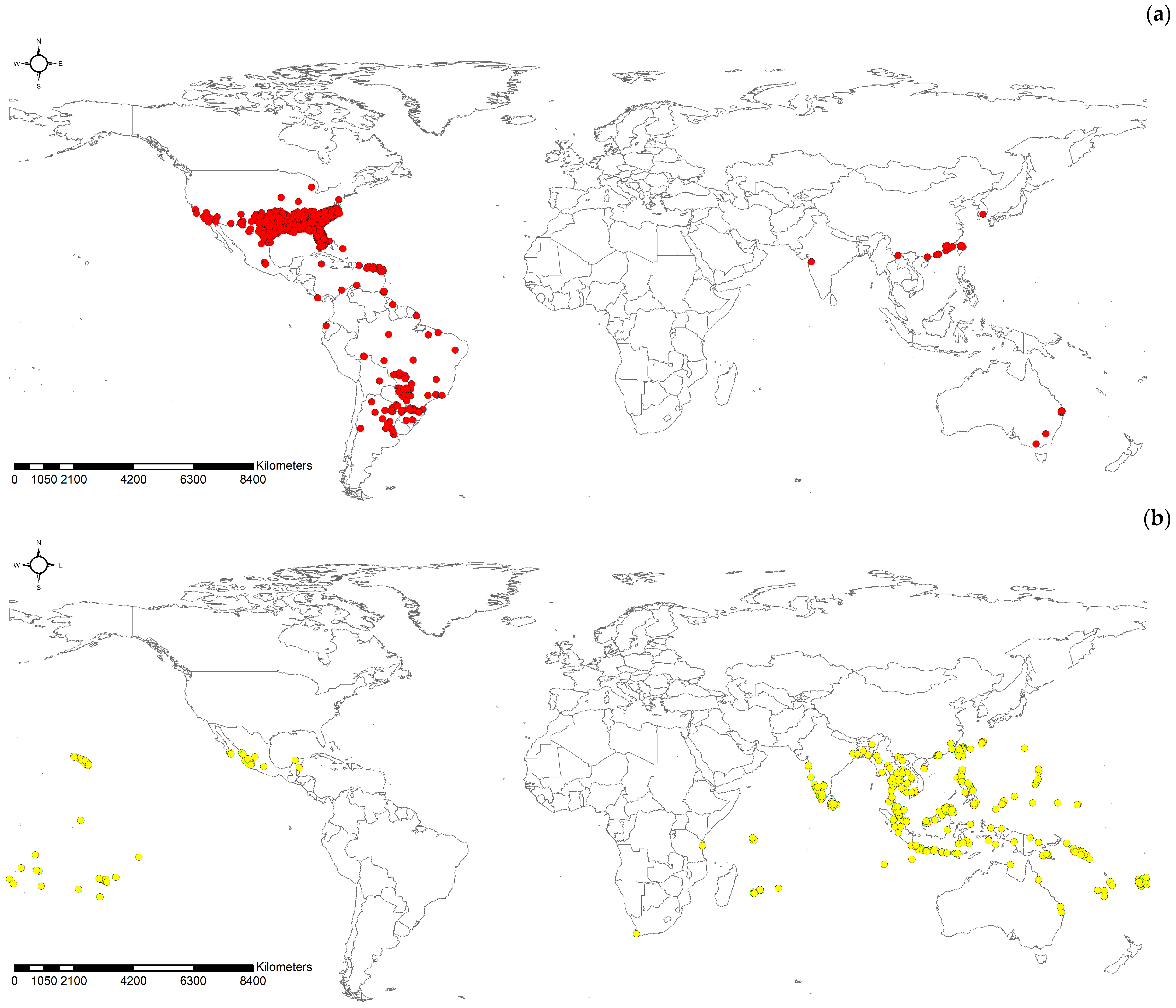
Figure 1. Global coordinating of occurrence data of (a) Solenopsis invicta (red dots) and (b) Anoplolepis gracilipes (yellow dots).
Applsci 12 10260 g001
Figure 2. Classification of potential presence and absence areas for S. invicta by each model and climate change scenario.
Applsci 12 10260 g002aApplsci 12 10260 g002b
Figure 3. Classification of potential presence and absence areas for A. gracilipes by each model and climate change scenario.
Applsci 12 10260 g003aApplsci 12 10260 g003b
Figure 4. Potential distribution of S. invicta by regressing occurrence possibility evaluated by each model and climate change scenario.
Applsci 12 10260 g004aApplsci 12 10260 g004b
Figure 5. Potential distribution of A. gracilipes by regressing occurrence possibility evaluated by each model and climate change scenario.
Applsci 12 10260 g005aApplsci 12 10260 g005b
Table 1. Selected model variables for each species.
SpeciesVariablesDescription
S. invictaBio1Annual Mean Temperature
Bio2Mean Diurnal Range
Bio3Isothermality
Bio5Max Temperature of Warmest Month
Bio8Mean Temperature of Wettest Quarter
Bio9Mean Temperature of Driest Quarter
Bio12Annual Precipitation
Bio14Precipitation Seasonality
Bio15Precipitation of Warmest Quarter
Elevation
A. gracilipesBio1Annual Mean Temperature
Bio2Mean Diurnal Range
Bio3Isothermality
Bio5Max Temperature of Warmest Month
Bio7Temperature Annual Range
Bio15Precipitation Seasonality
Bio16Precipitation of Wettest Quarter
Bio18Precipitation of Warmest Quarter
Bio19Precipitation of Coldest Quarter
Elevation
Table 2. Model performance metrics for both ant species.
SpeciesS. invictaA. gracilipes
ModelMaxEntRFMLPMaxEntRFMLP
AUC0.9490.9390.9110.9670.9400.894
pAUC1.9601.9701.9301.9301.9301.800
TSS0.9230.8790.8150.9060.8820.783
Accuracy0.9510.9410.9070.9300.9400.890
Sensitivity0.9730.9410.9060.9770.9100.944
Specificity0.9490.9380.9090.9290.9720.839
RF: Random Forest, and MLP: multi-layer perceptron.
Table 3. Areal ratio and average probability of potential distribution by models and climates.
SpeciesModelMaxEntRFMLP
ClimateCurrent2050Current2050Current2050
S. invicta% presence5.19%5.63%4.04%4.31%6.41%16.54%
Mean prob.0.3070.3190.7710.7560.7630.766
A. gracilipes% presence7.28%6.17%8.35%7.80%21.76%17.79%
Mean prob.0.3170.3490.7190.7390.7480.784
RF: Random Forest, and MLP: multi-layer perceptron. % presence: ratio of the number of cells counted in the area classified to presence to the whole number of worldwide cells. Mean prob.: average probability calculated in the area classified to presence.
Publisher’s Note: MDPI stays neutral with regard to jurisdictional claims in published maps and institutional affiliations.