Sparse Plane Wave Approximation of Acoustic Modes to Address Basis Mismatch

Abstract

Low-frequency sound field reconstruction in an enclosed space has many applications where the plane wave approximation of acoustic modes plays a crucial role. However, the basis mismatch of the plane wave directions degrades the approximation accuracy. In this study, a two-stage method combining ${\ell }_1$-norm relaxation and parametric sparse Bayesian learning is proposed to address this problem. This method involves selecting sparse dominant plane wave directions from pre-discretized directions and constructing a parameterized dictionary of low dimensionality. This dictionary is used to re-estimate the plane wave complex amplitudes and directions based on the sparse Bayesian framework using the variational Bayesian expectation and maximization method. Numerical simulations show that the proposed method can efficiently optimize the plane wave directions to reduce the basis mismatch and improve acoustic mode approximation accuracy. The proposed method involves slightly increased computational cost but obtains a higher reconstruction accuracy at extrapolated field points and is more robust under low signal-to-noise ratios compared with conventional methods.

1. Introduction

Recently, the reconstruction of a low-frequency sound field in an enclosed space has generated interest among researchers. It is significant for many applications, including sound field auralization [1], room equalization [2], sound field control [3,4,5], etc. The reconstruction problem usually involves interpolating the impulse responses at unmeasured positions from the impulse responses measured by a discrete set of microphones. The interpolation methodology can avoid the extensive experimental effort caused by dense point-by-point measurements. However, according to the study on the plenacoustic function [6], the Nyquist sampling theorem must be applied, requiring multiple microphone-based measurements for higher cut-off frequency. This contrasts with the goal of employing the minimum number of microphones to recover the sampled sound field faithfully.

The framework of compressive sensing (CS) [7,8] compensates for the lack of observation information by exploiting prior knowledge, so the inherent sparsity of a low-frequency enclosed sound field can help reduce the number of microphones. Under this framework, most methods formulate a physical propagation model and expand the limited set of measurements into finite-order elementary waves [9]. Commonly used elementary wave (or propagation model) includes the spherical harmonic function [10,11], plane wave (PW) [11,12,13,14,15,16,17], and free-field Green function [13]. The PW approximation is widely used because Vekua’s theory [18] shows that any homogeneous sound field in an enclosed convex region can be approximated by a finite number of PWs, independent of boundary conditions [19].

The current PW approximation methods can be classified into two types. The frequency-domain method [11,13,14,15,16] approximates the steady-state sound field by a finite sum of PWs for each frequency and uses the ${\ell }_1$-norm relaxation to solve the PW complex amplitudes (PWAs). In previous studies working with the frequency domain, different sparsity promoting regularizations were compared [13], and a two-step ${\ell }_1$-norm minimization method was developed by expressing PWs in the spherical harmonic domain to address the high mutual coherence of the sensing matrix when PWs are densely discretized [14]. The modal structure was incorporated into the PW model, and the proposed method could predict frequency response functions between the unmeasured source–receiver pairs [16]. The time-domain method [12,17] decomposes the homogeneous wave equation into the superposition of damped harmonic eigen-PWs. It first uses the matching pursuit or the rational fraction polynomials global curve fitting method to identify the acoustic modes, and then conducts the sparse PW approximation for each mode. Compared with the sound field in the frequency domain, the eigen-PWs of a single mode have substantially better sparsity, especially in rectangular enclosures. Therefore, this study focuses on the time-domain method’s PW approximation of acoustic modes.

However, the PW approximation has an inherent drawback in that the spatially continuous PW directions must be discretized, and regardless of how finely the directions are discretized, there is always a mismatch between the pre-discretized direction and the actual direction, which is referred to as the basis mismatch [20]. This will inevitably reduce the approximation accuracy. A dictionary or sensing matrix comprising dense PW directions is required to address this issue. This produces a high mutual coherence for the sensing matrix and has the disadvantage of increased computational time. A standard method used to tackle the basis mismatch in acoustics is to adaptively optimize pre-discretized grids based on parametric dictionary learning. For inhomogeneous sound field recording, a grid-pruning-based Newton’s method was utilized to optimize monopole positions [21]. Joint sparse recovery and a parametric dictionary learning problem were formulated based on the Bayesian framework for source localization [22]. While locating sources in a highly reverberant environment, the unknown room reflection energy ratio has been estimated. The parametric sparse Bayesian learning (SBL) has also been used to simultaneously estimate the unknown monopole positions and path loss exponent [23]. The pre-discretized grids near the sources were first selected, then a combination of the two-dimensional Newton optimization and a feedback mechanism was used to approximate the actual positions for beamforming [24]. In this study, PW discretization involves adaptively optimizing the propagating directions, including inclinations and azimuths, which have rarely been focused upon in previously published literature.

This study proposes a combined two-stage method to address the problem of basis mismatch in the PW approximation of acoustic modes. First, we use ${\ell }_1$-norm relaxation to solve the coarse PWAs, select dominant PW directions, and prune the other directions. Then, we use the extracted dominant directions to construct a low-dimensional parameterized dictionary that considers the PW directions as unknown parameters instead of densely discretizing the direction space to construct a high-dimensional known dictionary. We solve the PWAs and optimize the PW directions by applying SBL. This is facilitated by the variational Bayesian expectation and maximization (VBEM) technique [22,25,26], where the two-dimensional Newton optimization is derived to adaptively modify the inclinations and azimuths. A similar method has not been used in the field of sound reconstruction thus far. Numerical simulations show that the proposed method can reduce the basis mismatch in the PW approximation and improve the approximation accuracy compared with conventional methods, where the computational cost is slightly increased. Additional benefits of the proposed method include a high reconstruction accuracy at extrapolated field points outside the local measurement region and robustness under low signal-to-noise ratios (SNRs).

The paper is organized as follows. The problem of the PW approximation of acoustic modes is stated in Section 2, and the proposed two-stage method is described in Section 3. The simulation results are presented to validate the effectiveness of the proposed method in Section 4. A discussion is presented in Section 5, and conclusions are summarized in Section 6.

2. PW Approximation of Acoustic Modes

An acoustic mode function ${\psi }_{\mathit{n}}$ of order $\mathit{n}$ can be approximated by a finite sum of PWs sharing the same wavenumber $k_{\mathit{n}}$. The R-order approximation of ${\psi }_{\mathit{n}}$ at position $\mathit{r}={[x,y,z]}^{\mathrm{T}}$ is described as follows [12]:

$${\psi }_{\mathit{n}}\left(\mathit{r}\right)\approx \sum _{r=1}^R{w}_{\mathit{n},r}exp(-\mathrm{i}{k}_{\mathit{n}}{\mathit{s}}_r^{\mathrm{T}}\mathit{r}),$$

(1)

where the unit vector ${\mathit{s}}_r=\mathit{s}({\theta }_r,{\varphi }_r)={[sin{\theta }_{r}cos{\varphi }_r,sin{\theta }_{r}sin{\varphi }_r,cos{\theta }_r]}^{\mathrm{T}}$ represents the direction of the rth PW with inclination ${\theta }_r\in [0^{\circ },{180}^{\circ }]$ and azimuth ${\varphi }_r\in [0^{\circ },{360}^{\circ })$; ${(·)}^{\mathrm{T}}$ denotes the transpose operation; $k_{\mathit{n}}{\mathit{s}}_r$ is the rth wave vector of the $\mathit{n}$th mode; and $w_{\mathit{n},r}$ is the corresponding PWA. For a complex $k_{\mathit{n}}$ (damping wall), we assume that Equation (1) remains valid at locations far from the wall [12]. The problem is to estimate the values of ${\left\{w_{\mathit{n},r}\right\}}_{r=1}^R$ from limited measurements. Assuming that M samples are employed, Equation (1) can be converted to a matrix form as follows:

$${\mathit{\psi }}_{\mathit{n}}={\breve{\mathit{H}}}_{\mathit{n}}{\breve{\mathit{w}}}_{\mathit{n}},$$

(2)

where ${\breve{\mathit{H}}}_{\mathit{n}}$ is the $M\times R$ matrix, with its $(m,r)$th entry being $h_{\mathit{n},m}\left({\mathit{s}}_r\right)=exp(-\mathrm{i}{k}_{\mathit{n}}{\mathit{s}}_r^{\mathrm{T}}{\mathit{r}}_m)$, and ${\breve{\mathit{w}}}_{\mathit{n}}$ is the $R\times 1$ vector of the PWAs. The subscript ${(·)}_{\mathit{n}}$ is omitted below for simplicity of notation.

The discretized PW directions, $\mathcal{S}={\left\{{\mathit{s}}_r\right\}}_{r=1}^R$, are uniformly sampled on the surface of a unit sphere. Generally, $R>M$, and $\breve{\mathit{w}}$ can be solved as

$${\breve{\mathit{w}}}_{\mathrm{LS}}={\breve{\mathit{H}}}^{\mathrm{H}}{\left(\breve{\mathit{H}}{\breve{\mathit{H}}}^{\mathrm{H}}\right)}^{-1}\psi ,$$

(3)

where ${(·)}^{\mathrm{H}}$ denotes the conjugate transpose operation, which is the analytic solution of the underdetermined least-squares (LS) evaluated using the Tikhonov regularization. However, this solution tends to generate spatial aliasing artifacts. An alternative solution based on the CS framework exploits the prior knowledge that $\breve{\mathit{w}}$ is sparse. In this case, ${\ell }_1$-norm relaxation can be used to formulate an ${\ell }_1$-norm-regularized LS, also known as Lasso [27]. Its solution,

$${\breve{\mathit{w}}}_{\mathrm{L1}}=arg\underset{\breve{w}}{min}\{\frac{1}{2}\left|\right|\psi -\breve{\mathit{H}}\breve{\mathit{w}}{\left|\right|}_2^2+\lambda \left|\right|\breve{\mathit{w}}{\left|\right|}_1\},$$

(4)

where $\left|\right|·{\left|\right|}_2$ and $\left|\right|·{\left|\right|}_1$ represent the ${\ell }_2$-norm and ${\ell }_1$-norm, respectively, has few non-zero values and can be solved using iterative algorithms [28]. In our study, we applied the iterative reweighted least squares (IRLS) algorithm [29].

R is usually set to be considerably large to reduce the basis mismatch and obtain sufficiently dense PW directions. Thus, a high-dimensional dictionary was constructed. However, implementing this method is computationally expensive and even leads to failure of approximation.

3. Proposed Combined Two-Stage Method

In this section, we describe the proposed two-stage method combining ${\ell }_1$-norm relaxation and parametric SBL for the PW approximation of modes with reduced basis mismatch.

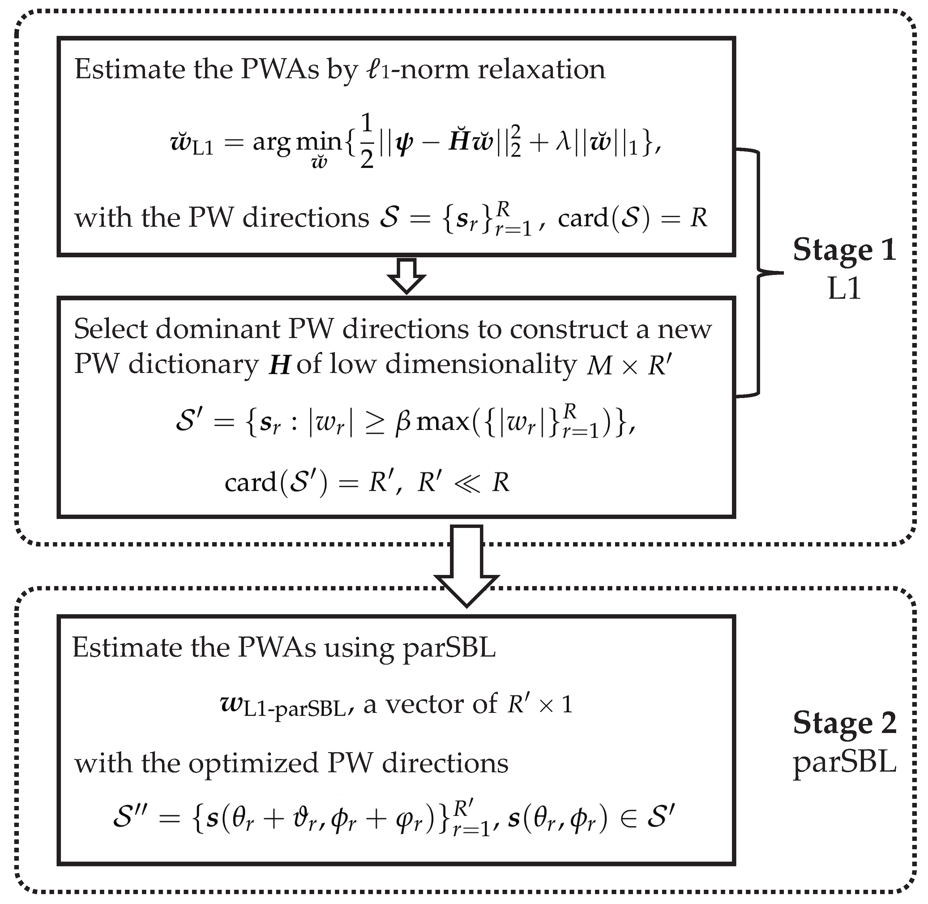
3.1. Stage 1: Selection of Dominant PW Directions Using ${\ell }_1$-Norm Relaxation

We used ${\ell }_1$-norm relaxation to estimate the PWAs $\breve{\mathit{w}}$ with respect to the R discretized PW directions in $\mathcal{S}$. We then selected the dominant directions ${\mathcal{S}}^{\prime }\subset \mathcal{S}$ whose corresponding absolute PWAs were greater than a certain percentage of the maximum, namely,

$${\mathcal{S}}^{\prime }=\{{\mathit{s}}_r:|w_r|\ge \beta max(\left\{\right|w_r{\left|\right\}}_{r=1}^R\left)\right\},\mathrm{card}\left({\mathcal{S}}^{\prime }\right)=R^{\prime },$$

(5)

where $\beta$ is the percentage, called the selection threshold, and $\mathrm{card}(·)$ denotes the cardinality of the set, that is, the number of selected directions. Owing to the sparsity of ${\breve{\mathit{w}}}_{\mathrm{L1}}$, $R^{\prime }\ll R$. We also used ${\mathcal{S}}^{\prime }$ to form a new dictionary $\mathit{H}$ of low dimensionality, $M\times R^{\prime }$, which is addressed in Stage 2. This stage is intended to reduce the calculation cost of the parametric SBL.

3.2. Stage 2: Estimation of PWAs and Directions Using Parametric SBL

3.2.1. Parameterized Dictionary

To avoid dense discretized PW directions, we explicitly modeled the dictionary with unknown inclinations and azimuths. The high dimensionality of the known dictionary can be reduced at the expense of introducing unknown parameters; therefore, we can apply the low-dimensional dictionary $\mathit{H}$ here. Let $\mathit{h}\left({\mathit{s}}_r\right)$ be the rth atom of the dictionary $\mathit{H}$ corresponding to the direction ${\mathit{s}}_r$. We assumed that the actual PW direction was ${\mathit{s}}_l\notin {\mathcal{S}}^{\prime }$ for some $l\in \{1,\dots ,L\}$ and that ${\mathit{s}}_{r_l}\in {\mathcal{S}}^{\prime }$ was the direction nearest to ${\mathit{s}}_l$. In this case, we can approximate the unknown $\mathit{h}\left({\mathit{s}}_l\right)$ using the multivariable Taylor expansion in the pre-discretized direction ${\mathit{s}}_{r_l}$ [30]:

$$\mathit{h}\left({\mathit{s}}_l\right)\approx \mathit{h}\left({\mathit{s}}_{r_l}\right)+{\mathit{h}}_{{\theta }_{r_l}}^{\prime }\left({\mathit{s}}_{r_l}\right)\times {\vartheta }_l+{\mathit{h}}_{{\varphi }_{r_l}}^{\prime }\left({\mathit{s}}_{r_l}\right)\times {\phi }_l,$$

(6)

where ${\mathit{h}}_{{\theta }_{r_l}}^{\prime }\left({\mathit{s}}_{r_l}\right)=\partial \mathit{h}\left({\mathit{s}}_{r_l}\right)/\partial {\theta }_{r_l}$, ${\mathit{h}}_{{\varphi }_{r_l}}^{\prime }\left({\mathit{s}}_{r_l}\right)=\partial \mathit{h}\left({\mathit{s}}_{r_l}\right)/\partial {\varphi }_{r_l}$, ${\vartheta }_l={\theta }_l-{\theta }_{r_l}$, and ${\phi }_l={\varphi }_l-{\varphi }_{r_l}$. Extending Equation (6), we construct the parameterized dictionary as follows:

$$\mathit{H}(\vartheta ,\phi )=\mathit{H}+{\mathit{H}}_{\theta }\mathrm{diag}\left(\vartheta \right)+{\mathit{H}}_{\varphi }\mathrm{diag}\left(\phi \right),$$

(7)

where

$$\begin{array}{cc}\hfill & {\mathit{H}}_{\theta }=[{\mathit{h}}_{{\theta }_1}^{\prime }\left({\mathit{s}}_1\right),\dots ,{\mathit{h}}_{{\theta }_{R^{\prime }}}^{\prime }\left({\mathit{s}}_{R^{\prime }}\right)],\hfill \\ \hfill & {\mathit{H}}_{\varphi }=[{\mathit{h}}_{{\varphi }_1}^{\prime }\left({\mathit{s}}_1\right),\dots ,{\mathit{h}}_{{\varphi }_{R^{\prime }}}^{\prime }\left({\mathit{s}}_{R^{\prime }}\right)],\hfill \\ \hfill & \vartheta ={[{\vartheta }_1,\dots ,{\vartheta }_{R^{\prime }}]}^{\mathrm{T}},\hfill \\ \hfill & \phi ={[{\phi }_1,...,{\phi }_{R^{\prime }}]}^{\mathrm{T}}.\hfill \end{array}$$

The problem in Equation (2) is reformulated as

$$\mathit{\psi }=\mathit{H}(\vartheta ,\phi )\mathit{w}.$$

(8)

The task is to estimate the PWAs $\mathit{w}$ and unknown parameters $\vartheta$ and $\phi$. This problem can be solved using a sparse Bayesian framework in a probabilistic manner.

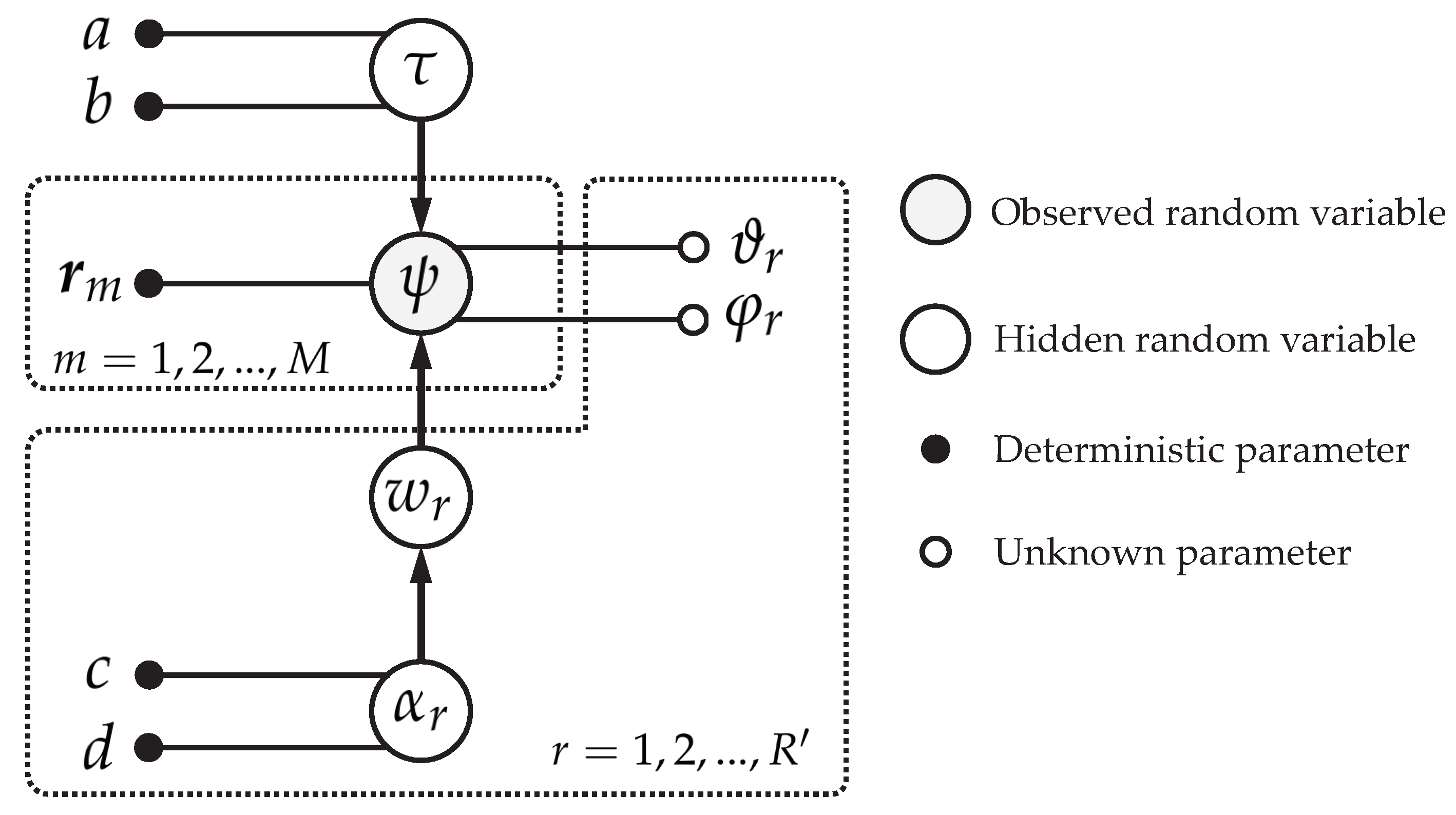
3.2.2. Probabilistic Model for SBL

From the SBL perspective, we attempt to find a function that maps arbitrary inputs $\mathit{r}$ (field point positions) to targets $\psi$ (acoustic mode values) based on training data ${\left\{\psi \left({\mathit{r}}_m\right)\right\}}_{m=1}^M$ (observations at samplings) to solve Equation (8) [26]. This function depends on a set of parameters $\mathit{w}$ (PWAs).

Within the sparse Bayesian framework, we first developed a probabilistic model. We assumed a complex, Gaussian-distributed additive noise $ϵ$ with zero mean and precision $\tau$ according to Equation (8). The likelihood function of the model $\mathit{\psi }=\mathit{H}(\vartheta ,\phi )\mathit{w}+ϵ$ then becomes

$$P\left(\psi \right|\mathit{w},\tau )=\mathcal{CN}\left(\psi \right|\mathit{H}(\vartheta ,\phi )\mathit{w},{\tau }^{-1}{\mathit{I}}_M),$$

(9)

where $\mathcal{CN}(·)$ indicates the complex Gaussian distribution and ${\mathit{I}}_M$ is an identity matrix of size M. A Gamma prior $\mathrm{Ga}(·)$ with parameters a and b is considered over $\tau$ in this study for tractable inference of $\tau$ described as follows:

$$P\left(\tau \right)=\mathrm{Ga}\left(\tau \right|a, b).$$

(10)

The components of PWAs $\mathit{w}$ are probabilistically independent of each other. Assuming that the rth entry follows a zero-mean, complex Gaussian prior with precision ${\alpha }_r$; this leads to the equation below,

$$P\left(\mathit{w}\right|\alpha )=\prod _{r=1}^{R^{\prime }}\mathcal{CN}\left(w_r\right|0,{\alpha }_r^{-1}).$$

(11)

Furthermore, a Gamma prior with parameters c and d is imposed on each hyperparameter ${\alpha }_r$, which yields

$$P\left(\alpha \right)=\prod _{r=1}^{R^{\prime }}\mathrm{Ga}\left({\alpha }_r\right|c, d).$$

(12)

Figure 1 shows the described probabilistic model of the variables and their hierarchical relationships.

Figure 1. Probabilistic model of parametric SBL represented as a Bayesian network (for conventional SBL, the parameters a, b, c, and d, are often set to be very small values, such as ${10}^{-6}$, in this study).

3.2.3. Hidden Random Variable Inference

We intended to obtain the posterior $P(\mathit{w},\tau ,\alpha |\psi )$ to evaluate inferences regarding hidden variables $\mathcal{H}=\{\mathit{w},\tau ,\alpha \}$ with the probabilistic model. However, the closed-form expression of the posterior is generally intractable owing to the difficulty in calculating the multidimensional integral when computing the model evidence $P\left(\psi \right)$. Therefore, we resorted to the VBEM method, which involves recursively approximating the posterior to infer $\mathcal{H}$ at the expectation step and optimizing $\vartheta$ and $\phi$ at the maximization step until convergence.

We assumed a distribution $Q\left(\mathcal{H}\right)$ with the factorized form in the expectation calculation step, that is, $Q\left(\mathcal{H}\right)=Q_1\left(\mathit{w}\right)Q_2\left(\tau \right)Q_3\left(\alpha \right)$. The posterior $P\left(\mathcal{H}\right|\psi )$ can then be approximated by minimizing the KL divergence between $P\left(\mathcal{H}\right|\psi )$ and $Q\left(\mathcal{H}\right)$ for given parameters $\vartheta$ and $\phi$, which is equivalent to solving the following equation

$$ln{\widehat{Q}}_j\left({\mathcal{H}}_j\right)={\mathbb{E}}_{Q(\mathcal{H}\setminus {\mathcal{H}}_j)}[lnP(\mathcal{H},\psi )],$$

(13)

where ${\mathbb{E}}_{Q(\mathcal{H}\setminus {\mathcal{H}}_j)}[·]$ represents the expectation of ${\prod }_{i\ne j}{Q}_i\left({\mathcal{H}}_i\right)$. Substituting the priors of $\mathcal{H}$, the updates of each $\mathcal{H}$ at the ith iteration can be summarized as follows [26]:

$$\begin{array}{cc}\hfill & {\mathit{\alpha }}^{\left(i\right)}=(c+1)\oslash [d+\mathrm{diag}({\mathit{\mu }}^{(i-1)}{\left({\mathit{\mu }}^{(i-1)}\right)}^{\mathrm{H}}+{\mathit{\Sigma }}^{(i-1)})],\hfill \end{array}$$

(14)

$$\begin{array}{cc}\hfill & {\tau }^{\left(i\right)}=\frac{a+M}{b+\left|\right|\mathit{\psi }-\mathit{H}(\mathit{\vartheta },\mathit{\phi }){\mathit{\mu }}^{(i-1)}{\left|\right|}_2^2+\mathrm{Tr}\left(\mathit{H}(\mathit{\vartheta },\mathit{\phi }){\mathit{\Sigma }}^{(i-1)}{\left(\mathit{H}(\mathit{\vartheta },\mathit{\phi })\right)}^{\mathrm{H}}\right)},\hfill \end{array}$$

(15)

$$\begin{array}{cc}\hfill & {\mathit{\Sigma }}^{\left(i\right)}={[{\tau }^{\left(i\right)}{\left(\mathit{H}(\mathit{\vartheta },\mathit{\phi })\right)}^{\mathrm{H}}\mathit{H}(\mathit{\vartheta },\mathit{\phi })+\mathrm{diag}\left({\mathit{\alpha }}^{\left(i\right)}\right)]}^{-1},\hfill \end{array}$$

(16)

$$\begin{array}{cc}\hfill & {\mathit{w}}^{\left(i\right)}={\mathit{\mu }}^{\left(i\right)}={\tau }^{\left(i\right)}{\mathit{\Sigma }}^{\left(i\right)}{\left(\mathit{H}(\mathit{\vartheta },\mathit{\phi })\right)}^{\mathrm{H}}\psi ,\hfill \end{array}$$

(17)

where ⊘ denotes the component-wise division, and $\mathrm{Tr}(·)$ represents the trace operation.

At the maximization step, we estimated the unknown parameters $\vartheta$ and $\phi$ separately by maximizing the expected log-likelihood for one parameter while keeping the other fixed. This is equivalent to solving the equation below,

$$\begin{array}{cc}\hfill & \widehat{\mathbf{x}}=arg\underset{\mathbf{x}}{min}\left\{\mathcal{L}\left(\mathbf{x}\right)\right\},\hfill \\ \hfill & \mathcal{L}\left(\mathbf{x}\right)=\left|\right|\mathit{\psi }-\mathit{H}\left(\mathbf{x}\right){\mathit{\mu }}^{\left(i\right)}{\left|\right|}_2^2+\mathrm{Tr}\left(\mathit{H}\left(\mathbf{x}\right){\mathit{\Sigma }}^{\left(i\right)}{\left(\mathit{H}\left(\mathbf{x}\right)\right)}^{\mathrm{H}}\right),\hfill \end{array}$$

(18)

where $\mathbf{x}$ represents $\vartheta$ or $\phi$. We used Newton’s method to solve this nonlinear problem. Accordingly, the single-step update of $\mathbf{x}$ is derived as

$$\begin{array}{cc}\hfill & {\mathbf{x}}^{\left(\mathrm{new}\right)}={\mathbf{x}}^{\left(\mathrm{old}\right)}-{\left[{\nabla }^2\mathcal{L}\left(\mathbf{x}\right)\right]}^{-1}{\nabla \mathcal{L}\left(\mathbf{x}\right)|}_{\mathbf{x}={\mathbf{x}}^{\left(\mathrm{old}\right)}},\hfill \\ \hfill & \nabla \mathcal{L}\left(\mathbf{x}\right)=2\Re [\mathrm{diag}\left({\mathit{\mu }}^{\left(i\right)}\right){\left({\mathit{H}}_{\mathbf{y}}\right)}^{\mathrm{T}}{(\mathit{H}\left(\mathbf{x}\right){\mathit{\mu }}^{\left(i\right)}-\psi )}^{*}+\mathrm{diag}\left({\mathit{\Sigma }}^{\left(i\right)}\right)\circ \mathrm{diag}\left({\left({\mathit{H}}_{\mathbf{y}}\right)}^{\mathrm{H}}\mathit{H}\left(\mathbf{x}\right)\right)],\hfill \\ \hfill & {\nabla }^2\mathcal{L}\left(\mathbf{x}\right)=2\Re \left[{\left[{\mathit{H}}_{\mathbf{y}}\mathrm{diag}\left({\mathit{\mu }}^{\left(i\right)}\right)\right]}^{\mathrm{H}}\left[{\mathit{H}}_{\mathbf{y}}\mathrm{diag}\left({\mathit{\mu }}^{\left(i\right)}\right)\right]\right]+2\mathrm{diag}\left(\mathrm{diag}\left({\mathit{\Sigma }}^{\left(i\right)}\right)\right)\circ \mathrm{diag}\left(\mathrm{diag}\left({\left({\mathit{H}}_{\mathbf{y}}\right)}^{\mathrm{H}}{\mathit{H}}_{\mathbf{y}}\right)\right),\hfill \end{array}$$

(19)

where $\{\mathbf{x},\mathbf{y}\}$ represents $\{\mathit{\vartheta },\mathit{\theta }\}$ or $\{\mathit{\phi },\mathit{\varphi }\}$; $\nabla \mathcal{L}\left(\mathbf{x}\right)$ and ${\nabla }^2\mathcal{L}\left(\mathbf{x}\right)$ denote the gradient and Hessian matrix of function $\mathcal{L}$ at $\mathbf{x}$, respectively; $\Re [·]$ is the real part of the argument; ${(·)}^{*}$ denotes the conjugate operation; ∘ refers to the Hadamard product; and the operation $\mathrm{diag}\left(\mathrm{diag}\right(·\left)\right)$ is equivalent to setting all entries of the matrix, except the diagonals, to zero. Note that the application of Newton’s method must ensure that the Hessian matrix ${\nabla }^2\mathcal{L}\left(\mathbf{x}\right)$ is positive definite; otherwise, Equation (19) must be modified accordingly [31]. In addition, each entry of $\mathbf{x}$ should be constrained within an appropriate interval to prevent excessive angle adjustments at the beginning of the iterative procedure, for example $[-{\mathrm{x}}_{\lim },{\mathrm{x}}_{\lim }]$. If $\mathrm{x}>{\mathrm{x}}_{\lim }$ or $\mathrm{x}<-{\mathrm{x}}_{\lim }$, we set $\mathrm{x}={\mathrm{x}}_{\lim }$ or $\mathrm{x}=-{\mathrm{x}}_{\lim }$. In our study, we set each entry of ${\mathbf{x}}_{\lim }$ to be the same and equal to $\lceil 2arcsin(D/2)\rceil$, where D is the average Euclidean distance between adjacent points ${\left\{{\mathit{s}}_r\right\}}_{r=1}^R$.

The second stage of the proposed method is summarized in Algorithm 1. Note that the solution ${\breve{\mathit{w}}}_{\mathrm{L1}}\in {\mathbb{C}}^{R\times 1}$ in Stage 1 is only used to select the dominant directions, and $\mathit{w}\in {\mathbb{C}}^{R^{\prime }\times 1}$ is initially assigned to ${\mathbf{0}}_{R^{\prime }}$. The results include the estimated PWAs and directions, which are denoted as $\{\mathit{w},{\mathcal{S}}^{″}\}$. Figure 2 shows a schematic illustration of the proposed method, L1-parSBL.

Figure 2. Flowchart of the combined two-stage method, L1-parSBL.

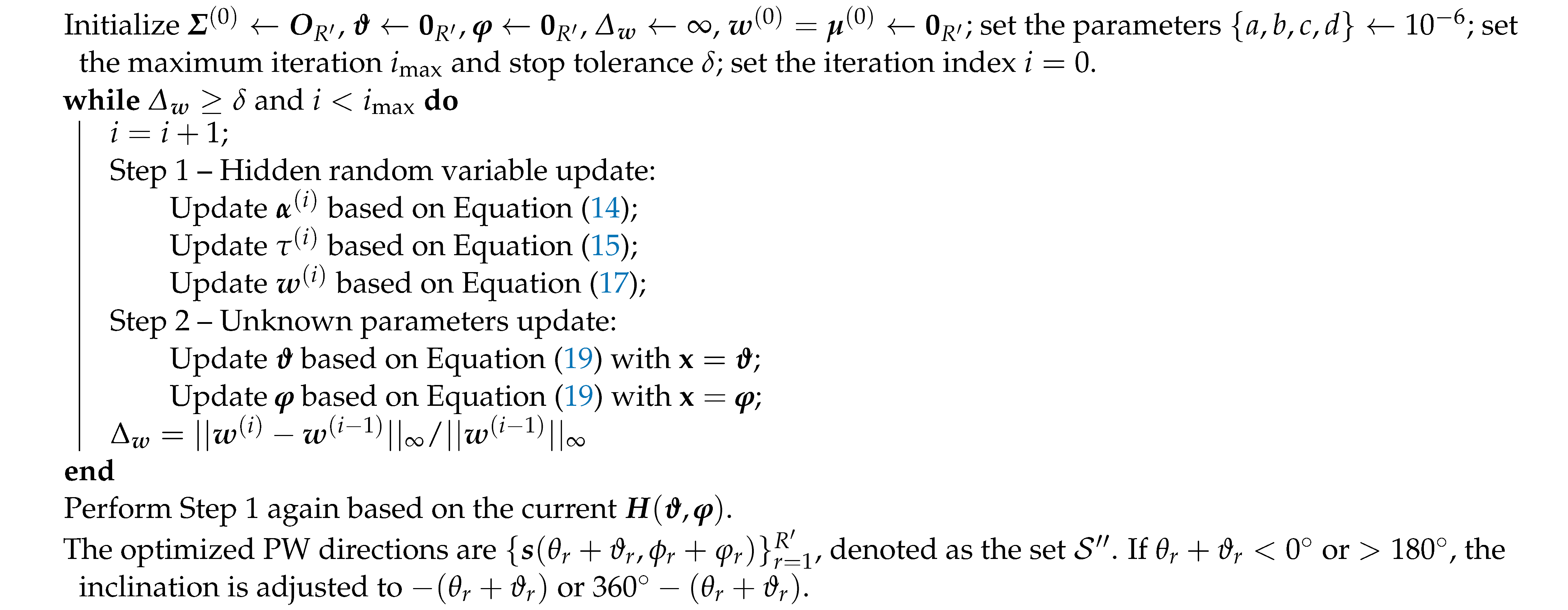
Algorithm 1: Stage 2: Estimation of PWs using parametric SBL (parSBL).

4. Simulations

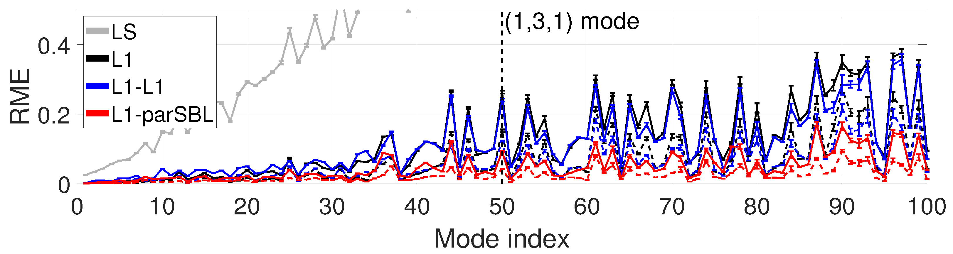
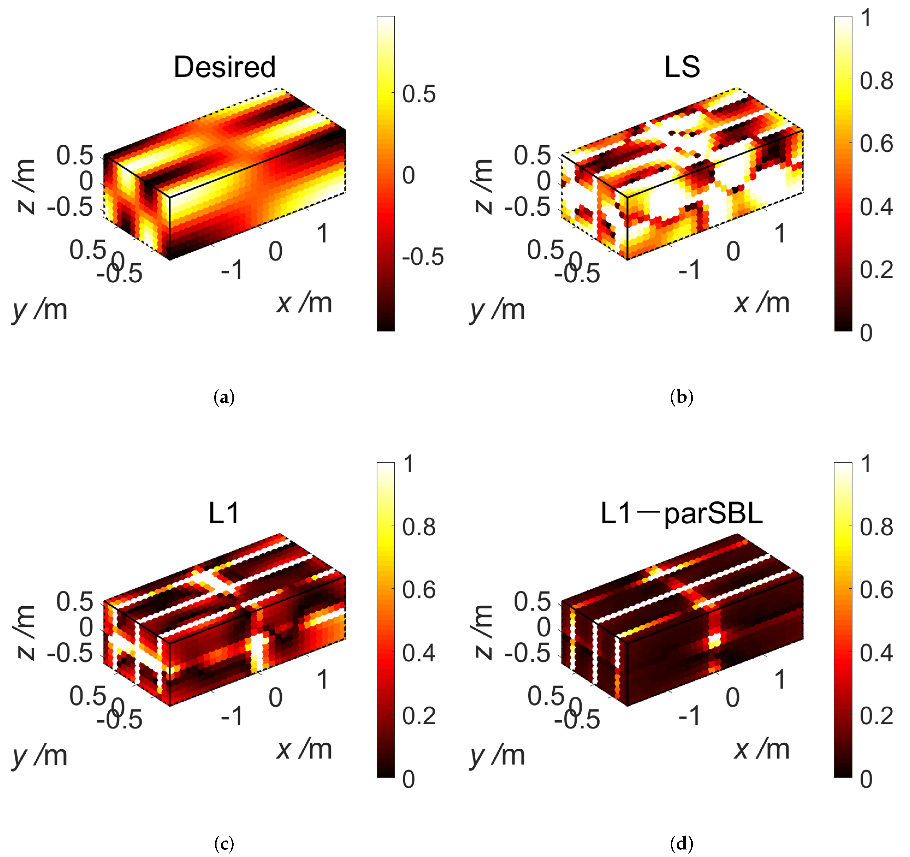
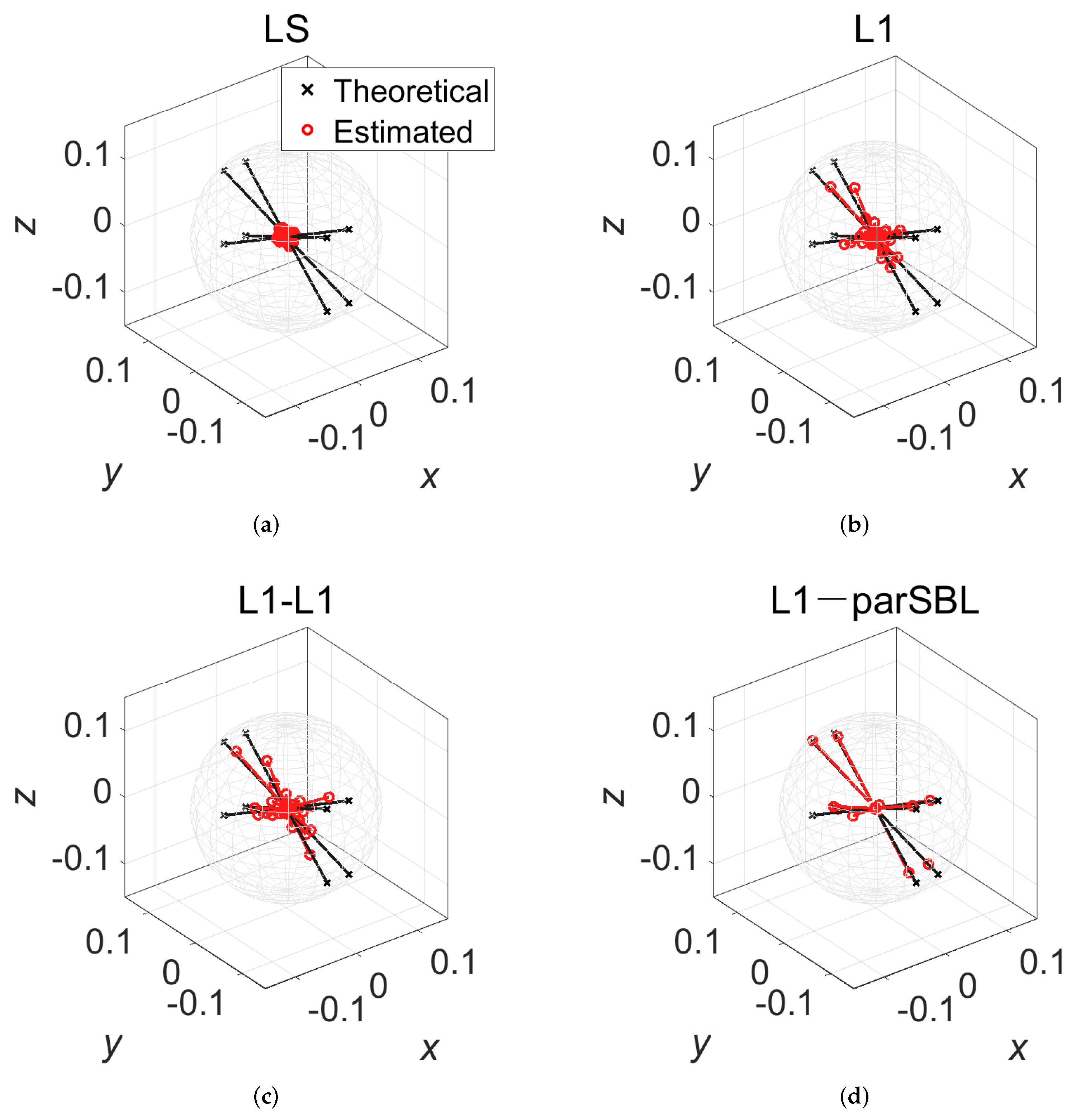
4.1. Validation Case: A Rigid-Walled Rectangular Enclosure

In our numerical simulation, we considered a rigid-walled rectangular enclosure of $3.7\mathrm{m}\times 1.8\mathrm{m}\times 1.2\mathrm{m}$. Each mode can be evaluated as a sum of eight PWs whose directions can be expressed analytically [32]. The results obtained by the proposed L1-parSBL were compared with conventional methods to examine the effectiveness and performance superiority of our method.

We employed 100 sets of $M=40$ randomly distributed samplings to measure the modes to eliminate the influence of random sampling positions. As it is difficult to calculate the estimation error of the PWAs directly, we used them further to reconstruct the mode and indirectly evaluate the relative mean error (RME) between the reconstructed mode values (${\psi }_{\mathrm{rec}}$) and those desired (${\psi }_{\mathrm{des}}$) at predefined field points in the volume as follows [14]:

$$\mathrm{RME}=\frac{\left|\right|{\mathit{\psi }}_{\mathrm{des}}-{\mathit{\psi }}_{\mathrm{rec}}{\left|\right|}_2}{\left|\right|{\mathit{\psi }}_{\mathrm{des}}{\left|\right|}_2},$$

(20)

In this case, the field points were set as $30\times 15\times 10$ equally-spaced grid points in the enclosure. The selection threshold $\beta$ was set to 0.1 because we clearly know that there are definite PWs objectively in this case. The discretized PW directions were obtained by solving the Thomson problem [33]. We examined two sets of pre-discretized PW directions of $R=400$ and 1000, and the corresponding ${\mathrm{x}}_{\lim }$s are ${11}^{\circ }$ and $7^{\circ }$, respectively.

Figure 3 shows the RMEs corresponding to the first 100 modes for different methods, with $R=400$ and 1000. The methods evaluated were LS, ${\ell }_1$-norm relaxation (L1), L1-L1, and the proposed L1-parSBL. L1-L1 denotes the method of selecting dominant PW directions based on L1 and re-estimating the PWAs based on the low-dimensional dictionary, according to L1. We observed that L1-parSBL outperformed the other methods, and even L1-parSBL with $R=400$ yielded better outcomes than the other methods with $R=1000$. All methods except LS provided comparable RMEs for low-order modes. LS exhibited very poor performance and could not provide an acceptable reconstruction for modes above the 22nd order (RME > 0.3). Although a maximum of eight PW directions exist, smaller eigenwavelengths relative to the enclosure size cause the mode shapes to become more complex and more sensitive to the basis mismatch for higher-order modes. Thus, the RMEs of the other methods were increased. L1-parSBL could reduce the basis mismatch and achieved a better RME because it optimized the PW directions in Stage 2. In addition, the RMEs of different higher-order modes were considerably different, corresponding to different mode shapes. Axial and tangential modes tended to be better reconstructed than oblique modes. For oblique modes, more sample data points were needed or samples needed to be arranged properly to capture sufficient spatial information.

Figure 3. (Color online) Relative mean error (RME) of different methods in different modes (—: $R=400$; - -: $R=1000$ ).

Specifically, we considered the high-order oblique mode (1, 3, 1) as an example to compare the approximation performance of these methods. Figure 4a shows the desired mode shape. Figure 4b–d plots the relative errors of the approximation at field points ($R=400$), $|{\mathit{\psi }}_{\mathrm{des}}-{\mathit{\psi }}_{\mathrm{rec}}|\oslash |{\mathit{\psi }}_{\mathrm{des}}|$, for LS, L1, and L1-parSBL, which achieved RME values of 0.73, 0.26, and 0.09, respectively. The result of L1-L1 was similar to that of L1 and is not shown here. It was observed that L1-parSBL produced a better reconstruction of the mode shape. In Figure 5a–d, note that the numbers of estimated PWs for LS and L1, $\{{\breve{\mathit{w}}}_{\mathrm{LS}},\mathcal{S}\}$ and $\{{\breve{\mathit{w}}}_{\mathrm{L1}},\mathcal{S}\}$, respectively, were both $R=400$; in contrast, for L1-L1, there existed only $R^{\prime }=23$ estimated PWs, $\{{\mathit{w}}_{\mathrm{L1}-\mathrm{L1}},{\mathcal{S}}^{\prime }\}$, whose directions were selected in Stage 1. Moreover, L1-parSBL yielded $R^{\prime }=23$ estimated PWs, $\{{\mathit{w}}_{\mathrm{L1}-\mathrm{parSBL}},{\mathcal{S}}^{″}\}$, whose directions were selected in Stage 1 and optimized in Stage 2. LS could not identify the actual PW directions because of which spatial aliasing artifacts were produced. The PWs could not be accurately estimated because of the basis mismatch, although L1 and L1-L1 could identify approximate directions. The proposed L1-parSBL efficiently optimized the PW directions to ensure that they were closer to the actual ones in Stage 2 and L1-parSBL estimated the PWAs more precisely than other methods. Similar results were obtained for the other modes as well. Thus, outcomes for only one mode are illustrated.

Figure 4. (Color online) Results of the PW approximation for the (1, 3, 1) mode with $R=400$. (a) Desired mode shape. (b–d) Spatial distribution of relative errors of the reconstructed mode when using (b) LS, (c) L1, and (d) L1-parSBL.

Figure 5. (Color online) Comparison between the theoretical and estimated PWs obtained using (a) LS ($R=400$), (b) L1 ($R=400$), (c) L1-L1 ($R^{\prime }=23$), and (d) L1-parSBL ($R^{\prime }=23$) for the (1, 3, 1) mode. The arrows indicate the PW directions, and their lengths are equal to the absolute PWAs.

The elapsed times of L1, L1-L1, and L1-parSBL for the PW approximation of the (1, 3, 1) mode are listed in Table 1. The computer included two Intel Xeon central processing units with two 2.20 GHz processors. For the same R, L1-parSBL required a slightly longer time as observed from Table 1. This was because in Stage 2, parSBL handled a very low-dimensional dictionary ($R^{\prime }\ll R$), which was constructed in Stage 1.

Table 1. Computational times based on 50 independent trials.

R	L1	L1-L1	L1-parSBL
400	0.95 s	0.96 s	1.17 s
1000	6.23 s	6.24 s	6.43 s

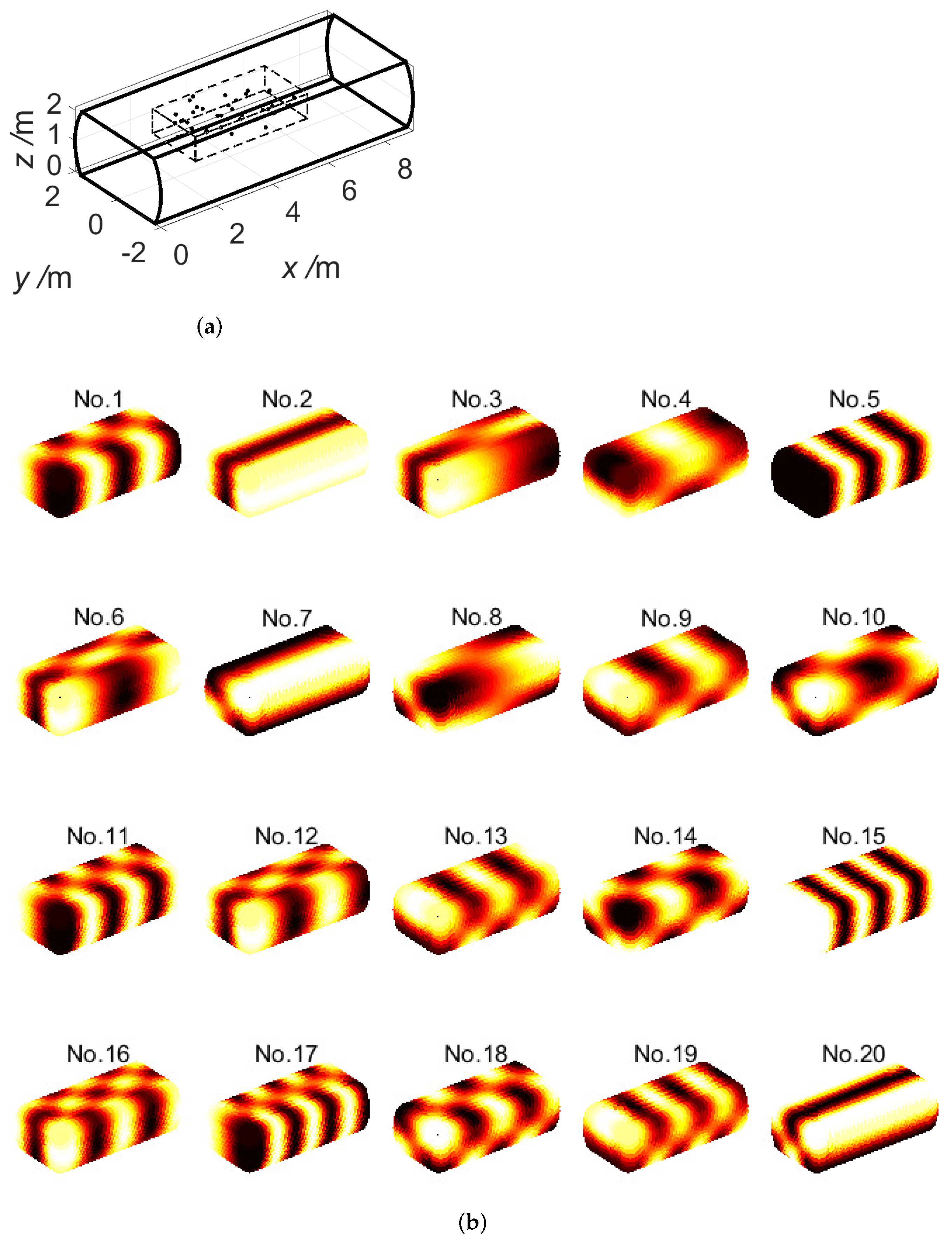
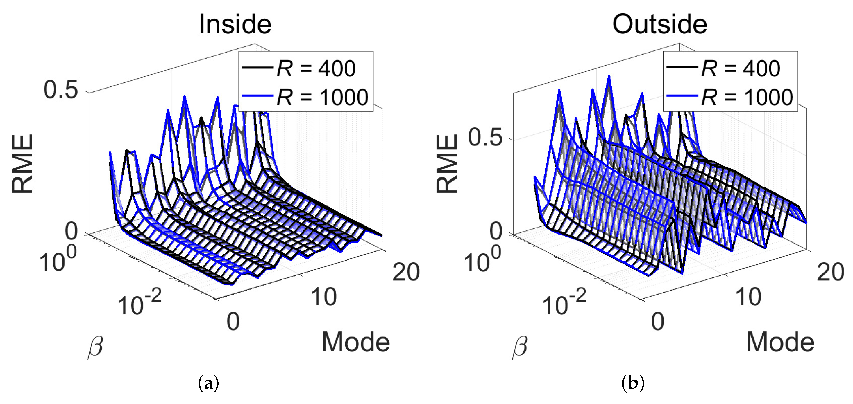
4.2. Case: An Aircraft Cabin with Damping Floor

In this subsection, we considered a more realistic enclosure environment for an aircraft cabin, as shown in Figure 6a. The floor was set as a damping boundary with an absorption coefficient $\alpha =0.1$. In practice, we generally focus more on local regions. Therefore, a virtual parallelepiped of $4\mathrm{m}\times 2\mathrm{m}\times 0.8\mathrm{m}$ with the center at ${[4,0,1.4]}^{\mathrm{T}}$ was defined as the sampling region. We used the Eigenfrequency study in the Pressure Acoustics, Frequency Domain physics interface in COMSOL Multiphysics for simulation. The vertices of the meshes inside the virtual parallelepiped region were chosen as the interpolated field points for assessment, and those outside the region were chosen as the extrapolated field points. We used 100 sets of $M=40$ samplings. Zero-mean, additive, Gaussian noise with an SNR of 25 dB was present during each sampling. We examined 20 modes around 107.5 Hz (the first-order blade-passing frequency) whose mode shapes are plotted in Figure 6b.

Figure 6. (Color online) (a) Geometry of the enclosure, with the dashed box denoting the virtual parallelepiped and the black dots representing the randomly distributed samplings. (b) Desired mode shapes of the 20 modes around 107.5 Hz.

Figure 7 shows the effect of the selection threshold $\beta$ on the reconstruction RME. We divided the interval $[{10}^{-3},{10}^{-0.3}]$ of $\beta$ into 20 grids which were equally-spaced in a logarithmic scale. It could be observed that the RME increased as $\beta$ increased, because there were fewer PW directions selected, leading to the lack of some necessary information. When $\beta$ was less than 0.1, the RME hardly changed with it, for both interpolated or extrapolated field points. However, with smaller $\beta$, more trivial PW directions were selected. Thus, we selected $\beta$ to be 0.01 empirically, which meant that the PW directions whose absolute PWAs were less than 1% of the maximum absolute PWA were discarded.

Figure 7. (Color online) RME of L1-parSBL versus the selection threshold $\beta$ in different modes, (a) inside the virtual region (i.e., for interpolated field points) and (b) outside the virtual region (i.e., for extrapolated field points).

Figure 8 shows the RMEs of LS, L1, and L1-parSBL for the 20 modes inside and outside the virtual region, respectively, with $R=400$ and 1000. We observed that L1-parSBL achieved better RMEs than LS and L1 inside and outside the virtual region for the 20 modes. The RMEs of LS were all greater than 0.5, and L1 could obtain RMEs below 0.3 under four modes for the extrapolated field points outside the region. In contrast, L1-parSBL achieved acceptable reconstruction errors (RME < 0.3) for 13 modes. We also found that the denser discretized PW directions hardly improved the RME in this case. Additionally, the RMEs of different modes were very different, especially for the extrapolated field points outside the virtual region. This was because samplings were distributed in the local region and these samplings could not obtain sufficient spatial information for some modes. For example, for modes “No. 3” and “No. 8” of Figure 6b, the virtual region mainly included their nodal planes, so it was difficult for the samplings to capture the effective information of the mode shapes. Therefore, the estimated PWs lead to poor reconstruction accuracy outside the virtual region.

Figure 8. (Color online) RME of LS, L1, and L1-parSBL in different modes (—: $R=400$; - -: $R=1000$), (a) inside the virtual region and (b) outside the virtual region.

Specifically, we considered the mode at approximately 106.5 Hz (closest to 107.5 Hz) as an example. Corresponding desired mode shape is plotted as the 12th subgraph in Figure 6b.

The effects of M (the number of sample data points) and SNR on the reconstruction accuracy of LS, L1, and L1-parSBL were analyzed. Figure 9a shows that the RMEs inside and outside the virtual region increased as M decreased for LS, L1, and L1-parSBL, respectively. Although the RMEs inside the region for the three methods were close, L1-parSBL had the lowest reconstruction errors. Both L1 and L1-parSBL could provide acceptable outcomes with $M=10$ samplings, but according to the error bar curves, specific sampling positions had significant impact. The proposed L1-parSBL achieved much better RMEs than LS and L1 when sufficient number of samples were used for the extrapolated field points. Based on Figure 9b, the RMEs inside and outside the virtual region increased as SNR decreased for LS, L1, and L1-parSBL, respectively. LS and L1 failed to reconstruct the mode shape outside the region (RME > 0.5) when SNR is below 25 dB. However, L1-parSBL still obtained the average RME of 0.5 at 15 dB. For interpolated field points, L1-parSBL could provide RME of 0.34 at 5 dB, whereas the RMEs of LS and L1 were basically more than 0.5 at 10 dB. Although only one mode outcome is illustrated here, similar results were obtained for the other modes as well.

Figure 9. (Color online) RME of LS, L1, and L1-parSBL (—: Inside; - -: Outside ) (a) versus M (the number of samplings) with SNR = 25 dB, and (b) versus SNR with $M=40$ for the mode at approximately 106.5 Hz with $R=400$.

Figure 10 presents the plots of the estimated PWs of LS, L1, and L1-parSBL under different SNRs for the “No. 12” mode at approximately 106.5 Hz by using a set of randomly distributed samplings ($R=400$). Note that there are no analytical PWs for this cabin case. The 12th subgraph in Figure 6b reveals that the mode shape had a significant characteristic of sparse PW superposition. There was no change in the modal values along the z-axis, regardless of the damping floor, indicating that the corresponding PWs of the mode were mainly concentrated on the equator of the unit sphere. It can be seen that LS could not identify sparse PWs. When SNR was 30 dB, the estimated PWs of LS barely exhibited four energy highlands around the equator. For lower SNRs, the estimated PWs distorted severely. A comparison between L1 and L1-parSBL shows that they both estimated PWs well at 30 dB. For lower SNRs, L1 obtained numerous PW artifacts that deviated from the equator. In contrast, the PWs estimated by L1-parSBL under different SNRs were similar; this reflected the robustness of L1-parSBL to some degree. At SNR = 10 dB, the PW estimation error of L1-parSBL was large. This could be partly attributed to the first stage estimate being wrong; thus, Stage 2 achieved no good results. L1-parSBL eliminated many artifacts selected in Stage 1 and significantly improved the reconstruction accuracy.

Figure 10. (Color online) Estimated PWs under different SNRs for the mode at approximately 106.5 Hz when using LS, L1, and L1-parSBL ($R=400$). (a–c) SNR = 30 dB. (d–f) SNR = 20 dB. (g–i) SNR = 10 dB.

5. Discussion

The proposed L1-parSBL was used in this study to address the adverse effect of the basis mismatch in PW discretization and improve the approximation accuracy of acoustic modes compared with conventional methods. L1-parSBL suffered from smaller reconstruction errors at extrapolated field points outside the region in a local sampling region because it estimated the corresponding PWs more precisely.

Note that no sparsity was assumed in Equation (1), and the finite sum of Equation (1) was an approximation required for computation [12]. The sparsity depends on the consistency between the enclosure geometry and the physical propagation model employed. For example, a cylindrical cavity will barely have a sparse representation with PWs (except in the z-axis) because PWs do not sparsely represent Bessel functions. The performance of CS-based methods deteriorates when the PWs of an acoustic mode are not very sparse. In this case, the selection threshold $\beta$ should be set with further insight [34,35].

The randomly distributed samplings must be arranged such that sufficient information of the sound field is captured. In addition, Stage 2 depended on the results of Stage 1. If the estimation was wrong in Stage 1 (for example, due to low SNR), it might be difficult to obtain good results in Stage 2. The IRLS was used here to calculate the coarse PWAs, ${\breve{\mathit{w}}}_{L1}$, in the first stage. Other algorithms need to be compared to evaluate an optimal paradigm, especially in terms of robustness.

6. Conclusions

We proposed a two-stage method, L1-parSBL, that combines ${\ell }_1$-norm relaxation with parametric SBL for the PW approximation of acoustic modes to reduce the adverse effect of basis mismatch. The first stage was used to select the sparse dominant PW directions from pre-discretized directions. The second stage was performed under the Bayesian framework to reformulate a parameterized dictionary of low dimensionality to re-estimate PWAs while optimizing the PW directions to approximate the actual directions. Numerical simulations were conducted using two models of an enclosure. The proposed L1-parSBL achieved a considerably higher approximation accuracy of acoustic modes than LS, L1, and L1-L1 for the rectangular enclosure with rigid walls. Based on an analysis of its (1, 3, 1) mode, it was illustrated that L1-parSBL could efficiently optimize the PW directions to reduce the effect of basis mismatch, albeit at the cost of a slightly increased computation time. A local measurement region was examined considering an enclosed aircraft cabin with a damping boundary. The results showed that L1-parSBL outperformed LS and L1, especially for extrapolated field points outside the region. L1-parSBL also exhibited much better robustness in low-SNR cases. The proposed L1-parSBL can further assist in enhancing the performance of reconstruction for sound fields, and related experimental work will be performed as part of future research.

References

- Murillo Gómez, D.M.; Astley, J.; Fazi, F.M. Low frequency interactive auralization based on a plane wave expansion. Appl. Sci. 2017, 7, 558. [Google Scholar] [CrossRef]
- Mazur, R.; Katzberg, F.; Mertins, A. Robust room equalization using sparse sound-field reconstruction. In Proceedings of the ICASSP 2019–2019 IEEE International Conference on Acoustics, Speech and Signal Processing (ICASSP), Brighton, UK, 12–17 May 2019. [Google Scholar]
- Bai, M.; Hsu, H.; Wen, J. Spatial sound field synthesis and upmixing based on the equivalent source method. J. Acoust. Soc. Am. 2014, 135, 269–282. [Google Scholar] [CrossRef]
- Jin, W.; Kleijn, W. Theory and design of multizone soundfield reproduction using sparse methods. IEEE/ACM Trans. Audio Speech Lang. Process. 2015, 23, 2343–2355. [Google Scholar]
- Caviedes-Nozal, D.; Heuchel, F.; Brunskog, J.; Riis, N.; Fernandez-Grande, E. A Bayesian spherical harmonics source radiation model for sound field control. J. Acoust. Soc. Am. 2019, 146, 3425–3435. [Google Scholar] [CrossRef]
- Ajdler, T.; Sbaiz, L.; Vetterli, M. The plenacoustic function and its sampling. IEEE Trans. Signal Process. 2006, 54, 3790–3804. [Google Scholar] [CrossRef]
- Candès, E.J.; Wakin, M.B. An introduction to compressive sampling. IEEE Signal Process. Mag. 2008, 25, 21–30. [Google Scholar] [CrossRef]
- Gerstoft, P.; Mecklenbräuker, C.F.; Seong, W.; Bianco, M.J. Introduction to compressive sensing in acoustics. J. Acoust. Soc. Am. 2018, 143, 3731–3736. [Google Scholar] [CrossRef] [Green Version]
- Koyama, S. Sparsity-based sound field reconstruction. Acoust. Sci. Technol. 2020, 41, 269–275. [Google Scholar] [CrossRef]
- Wang, Y.; Chen, K. Compressive sensing based spherical harmonics decomposition of a low frequency sound field within a cylindrical cavity. J. Acoust. Soc. Am. 2017, 141, 1812–1823. [Google Scholar] [CrossRef]
- Wang, Y.; Chen, K. Sound field reconstruction within an entire cavity by plane wave expansions using a spherical microphone array. J. Acoust. Soc. Am. 2017, 142, 1858–1870. [Google Scholar] [CrossRef] [PubMed]
- Mignot, R.; Chardon, G.; Daudet, L. Low frequency interpolation of room impulse responses using compressed sensing. IEEE/ACM Trans. Audio Speech Lang. Process. 2014, 22, 205–216. [Google Scholar] [CrossRef] [Green Version]
- Antonello, N.; De Sena, E.; Moonen, M.; Naylor, P.A.; Van Waterschoot, T. Room impulse response interpolation using a sparse spatio-temporal representation of the sound field. IEEE/ACM Trans. Audio Speech Lang. Process. 2017, 25, 1929–1941. [Google Scholar] [CrossRef] [Green Version]
- Wang, Y.; Chen, K. Sparse plane wave decomposition of a low frequency sound field within a cylindrical cavity using spherical microphone arrays. J. Sound Vib. 2018, 431, 150–162. [Google Scholar] [CrossRef]
- Verburg, S.A.; Fernandez-Grande, E. Reconstruction of the sound field in a room using compressive sensing. J. Acoust. Soc. Am. 2018, 143, 3770–3779. [Google Scholar] [CrossRef] [PubMed]
- Fernandez-Grande, E. Sound Field Reconstruction in a Room from Spatially Distributed Measurements. In Proceedings of the 23rd International Congress on Acoustics, Aachen, Germany, 9–13 September 2019; pp. 4983–4990. [Google Scholar]
- Pham Vu, T.; Hervé, L. Low frequency sound field reconstruction in a non-rectangular room using a small number of microphones. Acta Acust. 2020, 4, 5. [Google Scholar] [CrossRef]
- Vekua, I. New Methods for Solving Elliptic Equations; North-Holland Publishing Co.: Amsterdam, The Netherlands, 1967. [Google Scholar]
- Moiola, A.; Hiptmair, R.; Perugia, I. Plane wave approximation of homogeneous Helmholtz solutions. Z. Angew. Math. Phys. 2011, 62, 809–837. [Google Scholar] [CrossRef] [Green Version]
- Chi, Y.; Scharf, L.L.; Pezeshki, A.; Calderbank, A.R. Sensitivity to basis mismatch in compressed sensing. IEEE Trans. Signal Process. 2011, 59, 2182–2195. [Google Scholar] [CrossRef]
- Murata, N.; Koyama, S.; Takamune, N.; Saruwatari, H. Sparse sound field decomposition with parametric dictionary learning for super-resolution recording and reproduction. In Proceedings of the 2015 IEEE 6th International Workshop on Computational Advances in Multi-Sensor Adaptive Processing (CAMSAP), Cancun, Mexico, 13–16 December 2015; pp. 69–72. [Google Scholar]
- Wang, L.; Liu, Y.; Zhao, L.; Wang, Q.; Zeng, X.; Chen, K. Acoustic source localization in strong reverberant environment by parametric Bayesian dictionary learning. Signal Process. 2018, 143, 232–240. [Google Scholar] [CrossRef]
- You, K.; Guo, W.; Peng, T.; Liu, Y.; Zuo, P.; Wang, W. Parametric sparse Bayesian dictionary learning for multiple sources localization with propagation parameters uncertainty and nonuniform noise. IEEE Trans. Signal Process. 2020, 68, 4194–4209. [Google Scholar] [CrossRef]
- Yang, Y.; Chu, Z.; Yang, Y.; Yin, S. Two-dimensional Newtonized orthogonal matching pursuit compressive beamforming. J. Acoust. Soc. Am. 2020, 148, 1337–1348. [Google Scholar] [CrossRef]
- Beal, M. Variational Algorithms for Approximate Bayesian Inference; University of London: London, UK, 2004. [Google Scholar]
- Buchgraber, T. Variational Sparse Bayesian Learning: Centralized and Distributed Processing; Graz University of Technology: Graz, Austria, 2013. [Google Scholar]
- Tibshirani, R. Regression selection and shrinkage via the lasso. J. R. Stat. Soc. Ser. B 1994, 58, 267–288. [Google Scholar] [CrossRef]
- Rish, I.; Grabarnik, G.Y. Sparse Modeling: Theory, Algorithms, and Applications; CRC Press: Boca Raton, FL, USA, 2014. [Google Scholar]
- Hald, J. A comparison of iterative sparse equivalent source methods for near-field acoustical holography. J. Acoust. Soc. Am. 2018, 143, 3758–3769. [Google Scholar] [CrossRef] [Green Version]
- Yang, Z.; Xie, L.; Zhang, C. Off-grid direction of arrival estimation using sparse bayesian inference. IEEE Trans. Signal Process. 2013, 61, 38–43. [Google Scholar] [CrossRef] [Green Version]
- Fletcher, R. Practical Methods of Optimization, Volume 1: Unconstrained Optimization; John Wiley & Sons Ltd.: Hoboken, NJ, USA, 1980. [Google Scholar]
- Jacobsen, F.; Juhl, P.M. Fundamentals of General Linear Acoustics; John Wiley & Sons Ltd.: Hoboken, NJ, USA, 2013. [Google Scholar]
- Semechko, A. S2-Sampling-Toolbox. Available online: https://github.com/AntonSemechko/S2-Sampling-Toolbox (accessed on 16 December 2021).
- Piironen, J.; Vehtari, A. On the hyperprior choice for the global shrinkage parameter in the horseshoe prior. Artif. Intell. Stat. 2017, 54, 905–913. [Google Scholar]
- Bush, D.; Xiang, N. A model-based Bayesian framework for sound source enumeration and direction of arrival estimation using a coprime microphone array. J. Acoust. Soc. Am. 2018, 143, 3934–3945. [Google Scholar] [CrossRef] [PubMed] [Green Version]
Publisher’s Note: MDPI stays neutral with regard to jurisdictional claims in published maps and institutional affiliations. |
© 2022 by the authors. Licensee MDPI, Basel, Switzerland. This article is an open access article distributed under the terms and conditions of the Creative Commons Attribution (CC BY) license (https://creativecommons.org/licenses/by/4.0/).