Abstract
Although some traditional autoencoders and their extensions have been widely used in the research of intelligent fault diagnosis of rotating parts, their feature extraction capabilities are limited without label information. In response to this problem, this research proposes a hierarchical sparse discriminant autoencoder (HSDAE) method for fault diagnosis of rotating components, which is a new semi-supervised autoencoder structure. By considering the sparsity of autoencoders, a hierarchical sparsity strategy was proposed to improve the stacked sparsity autoencoders, and the particle swarm optimization algorithm was used to obtain the optimal sparsity parameters to improve network performance. In order to enhance the classification of the autoencoder, a class aggregation and class separability strategy was used, which is an additional discriminative distance that was added as a penalty term in the loss function to enhance the feature extraction ability of the network. Finally, the reliability of the proposed method was verified on the bearing data set of Case Western Reserve University and the bearing data set of the laboratory test platform. The results of comparison with other methods show that the HSDAE method can enhance the feature extraction ability of the network and has reliability and stability for different data sets.
1. Introduction
It is necessary to monitor the health of rotating parts and diagnose faults in complex working conditions because the working environment of high-speed rotating machinery is usually very harsh and complicated [1,2]. However, the artificially extracted features of traditional fault diagnosis methods are usually shallow features. Therefore, the research of intelligent fault diagnosis methods based on deep learning methods has received more and more attention. As an important branch of deep learning methods, supervised learning models with powerful feature extraction capabilities and data analysis capabilities have been applied to fault diagnosis [3,4]. Lin H et al. [5] used the strong non-mapping and self-learning ability of the neural network to build a BP neural network model to adapt to the state detection and fault diagnosis of rolling bearings and achieved satisfactory fault classification results. Tch CK et al. [6] studied the use of the ELM algorithm to classify bearing faults, and experiments show that the performance of the ELM algorithm is better than the BP algorithm. However, many studies have shown that simple supervised models are greatly affected by parameter adjustments and data input. In order to dig deeper into the deep rules of data, unsupervised learning models have begun to be widely studied.
Through the transformation of the original data to characterize the deep features of the sample, the common unsupervised learning network is used for feature extraction and data analysis [7]. In order to obtain good classification performance, the unsupervised model is often combined with the supervised model to form a semi-supervised model to achieve the purpose of adjusting the performance of the unsupervised model with the help of label information to obtain a reliable classification model. Wang FT et al. [8] proposed an enhanced depth feature extraction method based on Gaussian radial basis kernel function and autoencoder. The advantage of this method is that it can obtain higher test accuracy based on fewer iterations, but the disadvantage is that it requires manual experience to adjust network parameters. Zhu J et al. [9] proposed a new intelligent fault diagnosis method based on principal component analysis and deep belief network, which can realize reliable fault analysis based on original vibration data, but it is prone to overfitting.
As a typical unsupervised learning network, autoencoders have received extensive attention [10,11]. Zhao ZH et al. [12] proposed a frequency domain feature extraction autoencoder network, which uses an asymmetric autoencoder to learn the mapping relationship between time-domain signals and frequency-domain signals and obtains a better clustering effect on bearing data. Li K et al. [13] proposed a rolling bearing fault diagnosis method based on the sparse and nearest neighbor preservation theory deep extreme learning machine, which can unsupervised the deep law of data mining and supervised learning to solve the least square classification diagnosis. The results show that sparsity has a good ability to improve neural network performance. In addition, many studies have also shown that improving the sparsity of the autoencoder can enhance its network performance [14,15]. Moreover, the introduction of category information into the feature extractor can also enhance the effect of autoencoder feature extraction [16,17], but most of the existing research still does not consider this approach [18,19,20,21,22].
Due to the characteristics of deep neural networks, the selection of hyperparameters in the model is still very important [23,24,25]. To this end, genetic algorithm [26], cuckoo algorithm [27], gray wolf algorithm [28] and other methods have been used for hyperparameter optimization to improve the performance of neural networks. Zhou J et al. [29] researched and proposed a GA-SVM rolling bearing intelligent evaluation method based on feature optimization. The optimal parameter optimization model was obtained through a genetic algorithm, and high diagnostic accuracy was achieved. Chen J et al. [30] introduced the gray wolf optimization algorithm to optimize the key parameter smoothing factor of the model to obtain an ideal classification model. The results show that this method can achieve an effective diagnosis of bearing faults under different working conditions under a small sample training set. The above research shows that selecting appropriate hyperparameter optimization algorithms for different network structures can effectively improve the performance of the network model.
This study fully considers the sparsity, classification and hyperparameter selection of autoencoders and proposes a hierarchical sparse discriminant autoencoder (HSDAE) method. The proposed HSDAE method can improve the feature extraction performance of autoencoders from the aspects of network sparsity and classification and is used for fault diagnosis of rotating components under complex working conditions. A novel hierarchical sparse strategy was used to enhance the sparse connection between deep network layers, and at the same time, was combined with particle swarm optimization to obtain the optimal sparse hyperparameters to improve network sparsity. Class aggregation and class separability strategy were used as discriminative distance to enhance the classification ability of the network, thereby enhancing the feature extraction ability of the improved autoencoder. The proposed method was compared and analyzed with a variety of existing similar methods, and the results show the superiority of the proposed method.
The main innovations and contributions are as follows:
- (1)
- In this paper, a novel semi-supervised autoencoder (hierarchical sparse discriminant autoencoder) is proposed to extract features for fault diagnosis;
- (2)
- A novel hierarchical sparsity strategy is proposed to enhance the sparsity of autoencoder networks, combining class aggregation and class separability strategy to improve feature extraction performance;
- (3)
- Experimental comparative analysis verifies that the proposed method can achieve reliable fault diagnosis for rotating parts under complex working conditions;
The rest of this article is organized as follows: Firstly, Section 2 introduces the basic principles of stacked sparse autoencoders and particle swarm optimization algorithms. Secondly, Section 3 introduces the improvement of the original method in this study and the specific process of the proposed method. Section 4 then introduces the experimental results and verifies the effectiveness of the proposed method on the CWRU bearing data set and private-bearing data set. Finally, Section 5 is the conclusion.
2. Theoretical Background
2.1. Stacked Sparse Autoencoder
Autoencoder (AE) is a three-layer unsupervised neural network model, which is composed of an input layer, a hidden layer and an output layer, as shown in Figure 1. The core principle of AE is to make the output y equal to the input x and find a brief representation of the deep law of the original data through the encoding and decoding transformation of the hidden layer. The reconstruction error EAE of AE, whose input layer is m-dimensional, is expressed as:
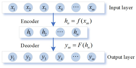
Figure 1.
The structure diagram of AE model.
Different from traditional autoencoders, the Sparse Auto Encoder (SAE) network adds KL divergence during the training process to limit the sparseness of the network to enhance the performance of the autoencoder [31]. Most of the nodes in the hidden layer are restricted by sparseness to suppress their activity, and only a small number of nodes are activated to explore the potential characteristics of the data. Hj(xi) indicates the activation level of the j-th neuron in the hidden layer, and the average activation level of m neurons in the hidden layer can be expressed as:
In order to better optimize the average activation degree, KL divergence was added to the SAE model. The KL divergence formula is as follows:
Then the loss function of traditional SAE is:
where m is the dimension of the input data, n is the number of neurons in the hidden layer and is the sparse penalty coefficient.
The Stacked Sparse Autoencoder (SSAE) connects multiple SAE structures by stacking, making full use of the characteristics of SAE to remove high-dimensional interference and extract low-dimensional features, enhancing the robustness of the autoencoder network, as shown in Figure 2 [32,33].
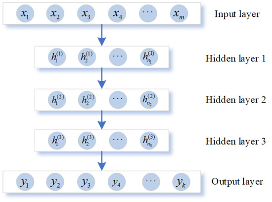
Figure 2.
The structure diagram of SSAE model.
2.2. Particle Swarm Optimization
The particle swarm optimization algorithm (PSO) is also called the bird swarm algorithm [34]. Its core principle is to obtain the best position of the bird swarm by simulating the predation behavior of the bird swarm. The algorithm designs a massless particle to simulate individuals in a flock of birds. Each particle has only two attributes: speed and position. Speed indicates the speed of the particle’s movement, and position indicates the direction of the particle’s movement. At the beginning of the predation behavior, the speed and position of each particle are random, and the fitness function is used as the basis for determining the optimal position during the movement.
Assuming that N particles are foraging together, the velocity and displacement of the n-th particle in the iterative process will be updated by Formulas (5) and (6):
where is a non-negative inertia factor used to balance the local and global optimization capabilities of particles. and are learning factors, which mainly control the influence of the individual extreme value and the global extreme value of the particle on the change in velocity. represents the random factor whose value is between 0 and 1, which enhances the particle’s ability to remove the local optimum with the help of perturbation. While and represent the local optimal position and the global optimal position of the particle swarm currently, respectively.
3. Proposed Methodology
3.1. Hierarchical Sparse Parameter Strategy
The loss function is very important in the training of the neural network. Choosing an appropriate neural network loss function can make the neural network model parameters converge to a value that can better describe the characteristics of the trained model [35]. The loss function is mainly divided into regression loss function and classification loss function, and different loss functions have different convergence characteristics. Therefore, the appropriate neural network loss function should be selected according to the purpose and nature of the neural network. Since the purpose of this research is to achieve classification, combined with the unsupervised nature of the autoencoder, the mean square error is selected as the basic loss function of the autoencoder. The traditional SSAE connects multiple identical SAE in series and uses the output of the previous SAE as the output of the next SAE. The loss function of traditional SSAE is:
In the formula, N is the number of stacked layers of SSAE and represents the number of neurons in the k-th layer.
It can be deduced from the formula that the traditional SSAE sparsity strategy is to give each layer of neurons the same expected activation ρ and the same sparsity parameter weight β, as shown in Figure 3a. Although it is impossible to reach the activation state shown in the figure during the training process, the figure shows the desired state of the network. This same sparse expectation may limit the learning ability of the deep sparse network to a certain extent.
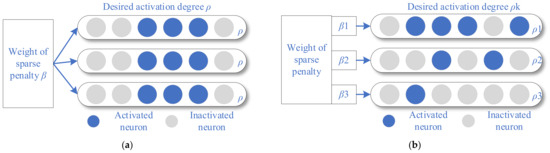
Figure 3.
The visual interpretation of hierarchical sparse strategy. (a) The schematic diagram of SSAE ordinary sparse strategy; (b) the schematic diagram of SSAE hierarchical sparse strategy.
However, considering that the number of neurons in each layer of a sparse network is usually not the same, the same sparse activation and sparse weight are not the optimal parameter selection. By aiming at this problem, a hierarchical sparsity strategy is proposed to randomize the sparsity activation and sparsity weights to expand the sparsity of the sparse network, as shown in Figure 3b. The loss function of the improved SSAE using the hierarchical sparse strategy is:
where is the sparse weight of the k-th layer of neurons and is the expected activation degree of the k-th layer.
Since the hierarchical sparse strategy is equivalent to increasing the randomness between hyperparameters, it is difficult to achieve the best results in manual tuning. Therefore, combined with the particle swarm optimization algorithm, the network sparsity is adaptively optimized to obtain reliable, optimal sparsity parameters.
3.2. Class Aggregation and Class Separability Strategy
The accuracy of the classifier in machine learning is largely affected by the extracted features. Furthermore, the more obvious the difference between the features, the better the classification effect. Thus, to improve the feature extraction capability of the autoencoder, a class aggregation and class separability strategy are introduced to limit feature mining from the data level to achieve better classification results.
The class aggregation and class separability strategy mean that the data points of each class are as compact as possible, and the distance between classes is as far as possible. Assuming that the same type of data point is drawn on a two-dimensional plane in the form of scattered points, there is usually a circle with the smallest radius to live all the data points. At this time, the center of this circle can be regarded as the fitting center point of this type of data, and the radius of this circle can be called the class radius r of this data type. According to this idea, assuming that there are N classes and the i-th class has group data , the class fitting center point and class radius of the i-th class are defined as:
At the same time, when there are N classes in total, the radius between classes and distance between classes is defined as:
When plotting data points of different classes on the same plane, the larger the distance between the fitting center points of each class, the better the class separation. Meanwhile, the smaller the class radius of each data class, the better the class aggregation. When the data points are distributed under these two conditions, it can be considered that the feature extraction effect is enhanced, as shown in Figure 4.
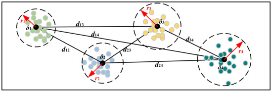
Figure 4.
The schematic diagram of class aggregation and class separability strategy.
The loss functions of class aggregation and class separability strategy are as follows:
where is the regular term and is the regular term coefficient. In the optimization process, ensure that takes the minimum value. In order to avoid negative optimization, the regular term can play a balancing role.
3.3. Parameter Optimization Strategy
3.3.1. Hierarchical Sparse Parameter Optimization with PSO
Using traditional PSO to optimize the hierarchical sparse parameters is easy to fall into the local optimum, so it is necessary to make some hyperparameters of PSO dynamic. The most important hyperparameters in PSO are the inertia factor and the learning factors and . mainly affects the range of optimizing ability, mainly affects self-learning ability and mainly affects group learning ability. In this regard, use the following formula to make the inertia factor and the learning factor dynamic.
where T is the total number of iteration steps, t is the number of current iteration steps, is the initial inertia factor, is the final inertia factor and is found to change linearly with the iteration process. and are the maximum learning factors and minimum learning factors in the iteration process, respectively.
3.3.2. Dynamic Optimization of Learning Rate
The learning rate mainly affects the convergence speed and direction of the loss function in the deep neural network training process. In order to solve the optimization problem of the learning rate , this paper adopts the inverse time learning rate decay method to optimize the learning rate dynamically, and the specific expression is as follows:
where T is the total number of iteration steps, and t is the current number of iteration steps.
3.4. HSDAE
The proposed HSDAE method combines SSAE with hierarchical sparsity strategy, class aggregation and class separability strategy and uses PSO to obtain the optimal sparsity hyperparameters. Its complete structure is shown in Figure 5.
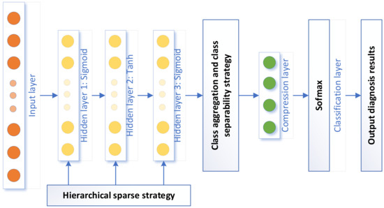
Figure 5.
The complete framework of the proposed method.
Unlike ordinary unsupervised autoencoders, HSDAE connects a layer of Softmax classifier after the last hidden layer to form a semi-supervised model. The loss function of the semi-supervised autoencoder model is as follows:
where refers to the dimension of the input data and refers to the dimension of the classification layer. The first half of the formula is the reconstruction function of the autoencoder, which retains the unique data reconstruction ability of the autoencoder; the second half of the formula is the cross-entropy function, which combines the label information with the unsupervised autoencoder to improve the network classification ability.
The loss function of the improved autoencoder after combining the above two strategies is:
in the formula, is the weighting factor to be set.
3.5. Overview of the Algorithm
In this study, the complete process is mainly divided into three parts, namely the PSO process, the training process and the testing process. Figure 6 is a complete flow chart of the proposed method. It should be noted that PSO is only used to optimize the sparse parameters to ensure network sparsity and speed up the optimization.
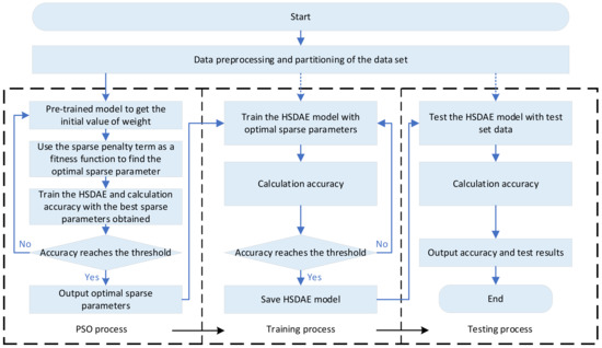
Figure 6.
The detailed flow chart of the proposed method.
The specific steps are as follows:
- Obtain the vibration signals of rotating machinery components, perform data preprocessing, convert them into frequency domain data and randomly divide the frequency domain data set into a training set and a testing set;
- Initialize HSDAE parameters and set key hyperparameters, such as the number of neurons in each layer, batch size, number of iterations, etc.;
- PSO parameter initialization, set the optimization boundary, inertia factor, learning factor, total number of particles and number of iterations;
- The HSDAE network uses the training set for pre-training to obtain the initial values of the variables in the network;
- Use the hierarchical sparse loss function as the fitness function of PSO to obtain the optimal sparse parameters. Use the optimal sparse parameters to train the HSDAE and calculate the accuracy. If the accuracy does not meet the conditions, return to step 4 to continue iterating until the accuracy threshold is met, and then the optimal sparsity parameter is output;
- Use the optimal sparse parameters to train the HSDAE, use the testing set to cross-validate, stop training and save the model when the accuracy meets the threshold;
- Use the testing set to test the model and output the diagnosis result.
4. Experimental Verification
4.1. Experimental Test 1
In order to verify the role of the HSDAE method in fault diagnosis of rotating machinery components, the rolling bearing public data set (CWRU) of Case Western Reserve University in the United States was selected for verification. The test platform is shown in Figure 7. In this study, the driving end signal with a sampling frequency of 48kHz was selected as the test data.
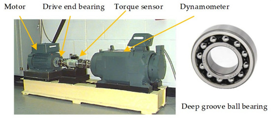
Figure 7.
The CWRU data set experiment platform.
The data under four load conditions of HP0, HP1, HP2 and HP3 are used in the CWRU data set. There are 10 types of faults in each load condition, including normal conditions. The experiment uses data augmentation to increase the number of samples, which means overlapping sampling with a smaller sample length. There are 600 groups of each type of failure sample, and each group has a sample length of 600. Half of the data are randomly selected as the testing set, and the remaining half is divided into the training set. The detailed division of the data set is shown in Table 1. The parameters of the PSO algorithm are consistent in this experiment; the optimization boundary is [0.0050, 0.4000], [, , , ] are set to [0.1, 0.01, 1.5, 1.5], respectively, the total number of particles is 20 and the number of iteration steps N is 100. For hierarchical sparse parameters [, , , , , ], the optimized dimension is 6, and for non-hierarchical sparse parameters [, ], the optimized dimension is 2. The parameter settings of HDSAE are shown in Table 2.

Table 1.
The test 1 data set detailed partition table.
Table 2.
The parameter settings of HDSAE in the CWRU data set.
4.1.1. Sparsity Verification
In order to verify the influence of the hierarchical sparsity strategy on the sparsity of the proposed method network neurons, the HSDAE method was tested on the above four data sets. The test experiment adopts the controlled variable method, one group uses hierarchical sparse parameters, and the other group uses non-hierarchical sparse parameters. The optimal sparsity parameter calculated by PSO is applied to the two groups, and finally, the KL divergence is used to measure the sparsity of each layer of neurons. Further, the smaller the KL divergence value, the smaller the average activation of neurons in the layer and the higher the sparsity. In order to ensure the reliability of the data, the average value of 20 test data is used for comparative analysis. Among them, the optimal hierarchical sparse parameter is [0.0679, 0.0448, 0.0396, 0.0398, 0.0336, 0.0522], and the optimal non-hierarchical sparse parameter is [0.1064, 0.0592].
The experimental results of HSDAE with hierarchical strategy and non-hierarchical strategy in data sets A, B, C and D are shown in Figure 8. Among them, in Figure 8a represents the KL divergence of the neurons in the x-th hidden layer. From the results in the figure, the hierarchical sparsity strategy has a significant impact on the sparsity of the first layer of neurons and the second layer of neurons because the KL divergence value of the hierarchical strategy is smaller than that of the non-hierarchical strategy. Although the KL divergence values of neurons in the third layer have little difference, the overall KL loss hierarchical strategy is smaller than that of the non-hierarchical strategy, as shown in Figure 8b. In short, the measurement results of the sparsity of neurons in each layer show that the hierarchical sparsity strategy can adjust the sparsity of each layer of a multi-layer network and enhance the sparsity of the network.
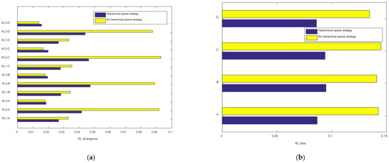
Figure 8.
The effect of hierarchical sparsity strategy on network sparsity. (a) KL divergence of neurons in each layer of different data sets; (b) KL divergence total loss for different data sets.
4.1.2. Class Aggregation and Class Separability Verification
In order to test the effects of class aggregation and class separability strategy, the t-SNE method is used to visualize the dimensionality reduction in the feature layer extracted by the model. The test methods are the complete HSDAE method and the HSDAE method without discriminant distance, using the optimal hierarchical sparse parameters. Then, the experimental results of the above two methods in data set C are selected and visualized by the t-SNE method. In Figure 9a, the original data overlaps and is chaotic, and the classification effect is not good. The HSDAE method without discriminant distance in Figure 9b can effectively separate all classes, and only a small amount of data is misclassified, but the uniformity and aggregation of the data points are poor. The HSDAE method in Figure 9c can not only separate all classes but also enhance the aggregation of each class. The data points are more evenly distributed and have good feature extraction capabilities. In summary, the class aggregation and class separation strategy can effectively enhance the aggregation of data classes and increase the distance between data classes. The experimental results reflect the excellent classification performance of the HSDAE method.
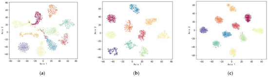
Figure 9.
Comparison of t-SNE diagrams of experimental results on data set C. (a) The t-SNE graph of data set C; (b) the t-SNE diagram of HSDAE features without discriminant distance; (c) the t-SNE diagram of HSDAE features.
4.1.3. Comparison Results of Different Methods
In order to analyze the performance of the HSDAE method, the proposed method was compared with the methods in the different literature for performance testing. The comparison methods mainly include the following four methods: LGSSAE [36], FDSAE [37], DisAE [38] and BNAE [39]. By considering the contingency of a single experiment, the following experimental results are the average results of 20 experiments.
It can be summarized from Table 3 that in the four data sets, the HSDAE method has the highest average diagnostic accuracy compared with other methods, and the highest average test accuracy can reach 99.39%. Because the load and speed of the four data sets are different, the comparison method shows different diagnostic performances on the four data sets, and the average test accuracy fluctuates more than 1%. The proposed method has a more stable performance on the four data sets, and the average test accuracy fluctuates less than 0.3%, indicating that it has a certain degree of robustness. Among the comparison methods, BNAE performed the worst, with an average accuracy of about 80%; LGSSAE and FDSAE achieved good results in data set A, but they did not perform well on data sets B, C and D; DisAE has achieved high test accuracy on multiple data sets, but the stability is not as good as HSDAE. In addition, from the standard deviation of the 20 experimental results, the standard deviation of the HSDAE method is the smallest, and its maximum standard deviation is only 0.0040, which shows strong stability compared with other methods.
Table 3.
The experimental results of different comparison methods in the CWRU data set.
To further illustrate the stability of the proposed method, 20 experimental results of data set D are selected, and a box plot is drawn, as shown in Figure 10. Moreover, the smaller the length of the blue box, the smaller the data fluctuation. Therefore, the LGSSAE, DisAE and HSDAE methods are more stable. However, the red “+” in the figure indicates the abnormal value in the data. Thus, the LGSSAE method and the DisAE method occasionally lose their diagnostic level. In general, the proposed method shows the best stability among all methods.
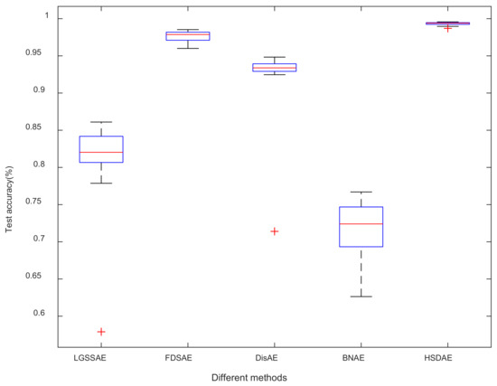
Figure 10.
Comparison of experimental results of different methods in data set D.
4.1.4. Visual Analysis of the Proposed Method
The confusion matrix can directly reflect the diagnosis results of the intelligent fault diagnosis method, so the confusion matrix is selected to analyze the HSDAE method further. It is the confusion matrix diagram of the 20th trial of the HSDAE method on data set A, as shown in Figure 11. It can be seen from the figure that, for the data of ten types of failures, the diagnostic accuracy of 99.27% can be achieved on the training set, and diagnostic accuracy of 99.1% can be achieved on the testing set. In the training set, categories 2, 4, 5, 6 and 9 all achieve 100% diagnostic accuracy, and the remaining categories have a small amount of misclassification. In the testing set, categories 1, 4, 6 and 9 achieved 100% diagnostic accuracy; except for categories 0 and 3, the number of misclassifications was very small. In conclusion, the diagnosis results show that the proposed method can achieve accurate fault diagnosis of rolling bearings.
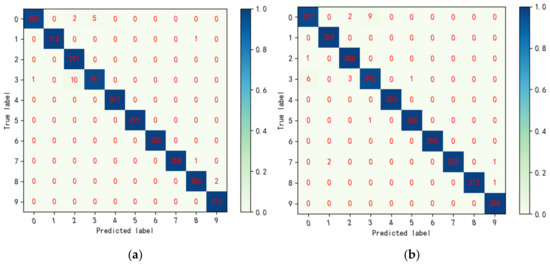
Figure 11.
Confusion matrix of the 20th experiment of HSDAE model on data set A. (a) The confusion matrix of the HSDAE model in the training set; (b) the confusion matrix of the HSDAE model in the testing set.
4.2. Experimental Test 2
In order to verify the diagnostic capabilities of the network model proposed in this paper, four sets of rolling bearing data with different speeds from the same private test platform in the author’s laboratory are selected for verification testing. In this study, the signal with a sampling frequency of 25.6 kHz was selected as the test data. The test platform is shown in Figure 12.
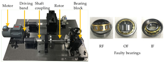
Figure 12.
The private data set experiment platform.
Similar to test one, the four types of fault data, including normal conditions under the conditions of rotation speed 900 rpm, 1100 rpm, 1300 rpm and 1500 rpm, are obtained, respectively. The length of each group of samples is 600, and the ratio of the testing set to the training set is the same as that of test one. The specific data set division is shown in Table 4. The test data also uses the frequency domain data processed by the data enhancement method. The PSO hyperparameter settings are the same as in experiment one. The parameters of HDSAE are shown in Table 5.
Table 4.
The test 2 data set detailed partition table.
Table 5.
The parameter settings of HDSAE in the private data set.
4.2.1. Sparsity Verification
Same as test one, the HSDAE method is used to verify the performance of the hierarchical sparsity strategy. With the help of the comparison results on the four data sets of E, F, G and H, the average KL divergence value of each layer of neurons is analyzed to verify the impact of the hierarchical sparsity strategy on sparsity. The data in the figure are the average of 20 trials to eliminate the randomness of the data. Among them, the optimal hierarchical sparse parameter is [0.0888, 0.1011, 0.1069, 0.1060, 0.0570, 0.0304], and the optimal non-hierarchical sparse parameter is [0.0561, 0.1009].
Figure 13 shows the experimental results of the network using the hierarchical sparse strategy and the network not using the hierarchical sparse strategy in the data sets E, F, G and H. Based on the observation of Figure 13a, the KL divergence values of the first layer of neurons and the third layer of neurons are significantly reduced under the action of the hierarchical sparse strategy. Although on the four data sets of E, F, G and H, the sparsity of the second layer of neurons is not affected by the hierarchical sparsity strategy. However, Figure 13b shows that the hierarchical sparse strategy has obvious sparse optimization for the overall HSDAE network. In summary, the experimental results of four sets of data show that the hierarchical sparsity strategy can indeed reduce the correlation between the sparsity of neuron layers and the number of layers in the multi-layer network.
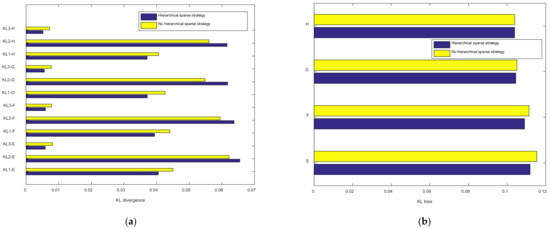
Figure 13.
The effect of hierarchical sparsity strategy on network sparsity. (a) KL divergence of neurons in each layer of different data sets; (b) KL divergence total loss for different data sets.
4.2.2. Class Aggregation and Class Separability Verification
Similarly, the t-SNE method is adopted to reduce the dimensionality of the feature layer and visualize it. The whole test process is the same as experiment one, and the optimal sparse parameter is still selected for the sparse parameter. The t-SNE comparison chart of a certain experimental result on the data set G is shown in Figure 14. Figure 14a illustrates that although the four types of faults in the original data set can be basically separated, each category still has a certain degree of dispersion; HSDAE without discriminant distance can extract the features of the original data, as shown in Figure 14b shows that the distance between the class and the class is obviously increased, but the aggregation within the class is slightly worse, and the data point distribution is messy. The HSDAE method has good class aggregation and class separability, as shown in Figure 14c; the distance between the class and the class center is large, and the data points are well-distributed. In summary, the t-SNE graph can reflect the class aggregation and class separability strategy, which can enhance the distance between classes, indicating that the proposed method has good feature extraction capabilities.
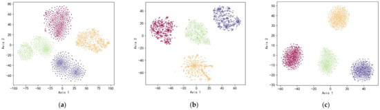
Figure 14.
Comparison of t-SNE diagrams of experimental results on data set G. (a) T-SNE graph of data set G; (b) the t-SNE diagram of HSDAE features without discriminant distance; (c) the t-SNE diagram of HSDAE features.
4.2.3. Comparison Results of Different Methods
Same as test 1, the proposed method with LGSSAE, FDSAE, DisAE, BNAE on four data sets of E, F, G and H are compared. Table 6 includes the average accuracy and standard deviation of the 20 experimental results of different methods on the above four data sets.
Table 6.
The experimental results of different comparison methods in the private data set.
It can be obtained from the table that the HSDAE method shows the best performance compared with other methods. On the private data set, BNAE performed the worst. It did not achieve 80% accuracy on the three data sets, and the maximum difference in average test accuracy reached 13.58%. The maximum difference in average accuracy between LGSSAE and DisAE is similar, but the overall accuracy of DisAE is higher than that of LGSSAE. FDSAE showed superior performance on the four data sets. The average accuracy is greater than 97.5%, and the maximum difference in average accuracy is only 1.35%. However, from the perspective of average test accuracy and standard deviation, the reliability and stability of FDSAE are still lower than the HSDAE method.
To further analyze the performance of HSDAE, select 20 experimental results of different methods on data set E and draw a box plot, as shown in Figure 15. It can be concluded from the figure that the stability of FDSAE, DisAE and HSDAE methods is significantly better than that of LGSSAE and BNAE methods. Although the median line of the FDSAE is similar to that of the HSDAE, its blue box is longer than that of the HSDAE, indicating that the stability of FDSAE is not as good as that of HSDAE. Therefore, HSDAE also shows excellent stability and reliability on private data sets.
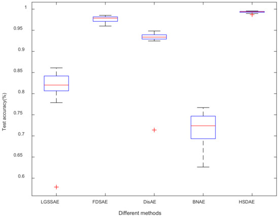
Figure 15.
Comparison of experimental results of different methods in data set E.
4.2.4. Visual Analysis of the Proposed Method
Similarly, a confusion matrix is used to analyze the fault diagnosis capability of the proposed method visually. Figure 16 is a confusion matrix diagram of the 20th trial of the HSDAE method on the data set H. It can be seen from the figure that for the four types of fault data, 100% diagnosis accuracy can be achieved on the training set and 99.87% diagnosis accuracy on the testing set. In the testing set, category 0, category 1 and category 3 achieve 100% accuracy, category 2 has four sets of data misclassification, and the recognition accuracy rate is 99.46%. In conclusion, the diagnosis results show that the proposed method can achieve accurate fault diagnosis of rolling bearings.
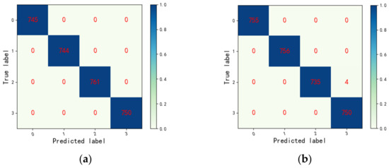
Figure 16.
Confusion matrix of the 20th experiment of HSDAE model on data set H. (a) The confusion matrix of the HSDAE model in the training set; (b) the confusion matrix of the HSDAE model in the testing set.
5. Conclusions
This paper proposes a hierarchical sparse discrimination autoencoder method for the intelligent diagnosis of rotating mechanical component faults. Through the experimental verification and analysis of the CWRU data sets and the private data sets, the following conclusions can be drawn:
- (1)
- The proposed hierarchical sparse strategy is used to optimize the SSAE, giving different sparse activation and sparse regularization weights to the neurons in each layer of SSAE, which enhances the randomness of the network sparseness and achieves better the diagnostic effect. Using the PSO to obtain the best sparse parameters adaptively driven by data can improve network sparseness and avoid the complexity of manual parameter selection;
- (2)
- The class aggregation and class separability strategy can effectively enhance the classification ability of the autoencoder network. It is proved from the side that the proposed method can optimize the feature extraction performance of the autoencoder;
- (3)
- Compared with other methods, the standard deviation of the HSDAE method proposed in this paper is small, and the fault diagnosis accuracy is high, which reflects the effectiveness, reliability and stability of the HSDAE method in fault diagnosis.
Regarding the future work direction, in this study, the hierarchical sparse strategy and discriminative distance are combined as the loss penalty term of the loss function. Therefore, specifying a better strategy is an important direction of subsequent research. In addition, the method proposed in this paper can only perform accurate fault diagnosis for the same distributed data set. In the future, the domain adaptive method will be further studied based on this method to realize the fault diagnosis for different distributed data sets.
Author Contributions
Conceptualization, M.Z.; methodology, M.Z.; software, M.Z.; validation, M.Z.; formal analysis, K.X.; investigation, J.L.; resources, S.L.; data curation, R.L. and K.X.; writing—original draft preparation, M.Z.; writing—review and editing, M.Z. and S.L.; visualization, M.Z.; supervision, R.L. and X.L.; project administration, S.L. and J.D.; funding acquisition, K.X., S.L. and Y.W. All authors have read and agreed to the published version of the manuscript.
Funding
This research was funded by the National Natural Science Foundation of China (51975276).
Institutional Review Board Statement
Not applicable.
Informed Consent Statement
Not applicable.
Data Availability Statement
There are no relevant statements for this research.
Acknowledgments
Thanks to all the participants who promoted the successful completion of this article, which was funded by the Special Project of National Key Research and Development Program of China (2020YFB1709801), the National Natural Science Foundation of China (51975276), and the Stability Support Project of Sichuan Gas Turbine Research Institute of AECC (WDZC-2020-4-7).
Conflicts of Interest
The authors declare no conflict of interest.
References
- Xu, K.; Li, S.; Li, R.; Lu, J.; Li, X.; Zeng, M. Domain Adaptation Network with Double Adversarial Mechanism for Intelligent Fault Diagnosis. Appl. Sci. 2021, 11, 7983. [Google Scholar] [CrossRef]
- Xu, K.; Li, S.; Li, R.; Lu, J.; Zeng, M. Deep domain adversarial method with central moment discrepancy for intelligent transfer fault diagnosis. Meas. Sci. Technol. 2021, 32, 124005. [Google Scholar] [CrossRef]
- Li, R.; Li, S.; Xu, K.; Lu, J.; Teng, G.; Du, J. Deep domain adaptation with adversarial idea and coral alignment for transfer fault diagnosis of rolling bearing. Meas. Sci. Technol. 2021, 32, 094009. [Google Scholar] [CrossRef]
- Li, R.; Li, S.; Xu, K.; Li, X.; Lu, J.; Zeng, M.; Li, M.; Du, J. Adversarial Domain Adaptation of Asymmetric Mapping with Coral Alignment for Intelligent Fault Diagnosis. Meas. Sci. Technol. 2021, 1–16. [Google Scholar] [CrossRef]
- Huo, L.; Zhang, X.Y.; Li, H.D. Bearing Fault Diagnosis Based on BP Neural Network. In Proceedings of the International Conference on Air Pollution and Environmental Engineering (APEE), Hong Kong, China, 26–28 October 2018. [Google Scholar]
- Teh, C.K.; Aziz, A.; Elamvazuthi, I.; Man, Z. Classification of Bearing Faults using Extreme Learning Machine Algorithm. In Proceedings of the 2017 IEEE 3rd International Symposium in Robotics and Manufacturing Automation (ROMA), Kuala Lumpur, Malaysia, 19–21 September 2017. [Google Scholar]
- Zhao, K.; Jiang, H.K.; Li, X.Q.; Wang, R.X. An optimal deep sparse autoencoder with gated recurrent unit for rolling bearing fault diagnosis. Meas. Sci. Technol. 2020, 31, 015005. [Google Scholar] [CrossRef]
- Wang, F.T.; Dun, B.S.; Liu, X.F.; Xue, Y.H.; Li, H.K.; Han, Q.K. An Enhancement Deep Feature Extraction Method for Bearing Fault Diagnosis Based on Kernel Function and Autoencoder. Shock Vib. 2018, 2018, 6024874. [Google Scholar] [CrossRef]
- Zhu, J.; Hu, T.Z.; Jiang, B.; Yang, X. Intelligent bearing fault diagnosis using PCA-DBN framework. Neural Comput. Appl. 2020, 32, 10773–10781. [Google Scholar] [CrossRef]
- Chen, S.; Yu, J.; Wang, S. One-dimensional convolutional auto-encoder-based feature learning for fault diagnosis of multivariate processes. J. Process Control 2020, 87, 54–67. [Google Scholar] [CrossRef]
- Deng, Z.; Li, Y.; Zhu, H.; Huang, K.; Tang, Z.; Wang, Z. Sparse stacked autoencoder network for complex system monitoring with industrial applications. Chaos Solitons Fractals 2020, 137, 109838. [Google Scholar] [CrossRef]
- Zhao, Z.; Li, L.; Yang, S.; Li, Q. A frequency domain feature extraction autoencoder and its application in fault diagnosis. China Mech. Eng. 2021, 32, 2468–2474. (In Chinese) [Google Scholar]
- Li, K.; Xiong, M.; Su, L.; Lu, L.; Chen, S. Research on Mechanical Fault Diagnosis Method Based on Improved Deep Extreme Learning Machine. J. Vib. Meas. Diagn. 2020, 40, 1120–1127. [Google Scholar]
- Jia, F.; Lei, Y.; Guo, L.; Lin, J.; Xing, S. A neural network constructed by deep learning technique and its application to intelligent fault diagnosis of machines. Neurocomputing 2018, 272, 619–628. [Google Scholar] [CrossRef]
- Sun, W.; Shao, S.; Zhao, R.; Yan, R.; Zhang, X.; Chen, X. A sparse auto-encoder-based deep neural network approach for induction motor faults classification. Measurement 2016, 89, 171–178. [Google Scholar] [CrossRef]
- Deng, S.; Du, L.; Li, C.; Ding, J.; Liu, H. SAR Automatic Target Recognition Based on Euclidean Distance Restricted Autoencoder. IEEE J. Sel. Top. Appl. Earth Obs. Remote Sens. 2017, 10, 3323–3333. [Google Scholar] [CrossRef]
- Liu, G.; Li, L.; Jiao, L.; Dong, Y.; Li, X. Stacked Fisher autoencoder for SAR change detection. Pattern Recognit. 2019, 96, 106971. [Google Scholar] [CrossRef]
- Chen, Z.; Li, W. Multisensor Feature Fusion for Bearing Fault Diagnosis Using Sparse Autoencoder and Deep Belief Network. IEEE Trans. Instrum. Meas. 2017, 66, 1693–1702. [Google Scholar] [CrossRef]
- Kong, D.; Yan, X. Adaptive parameter tuning stacked autoencoders for process monitoring. Soft Comput. 2020, 24, 12937–12951. [Google Scholar] [CrossRef]
- Lei, Y.; Jia, F.; Lin, J.; Xing, S.; Ding, S.X. An Intelligent Fault Diagnosis Method Using Unsupervised Feature Learning Towards Mechanical Big Data. IEEE Trans. Ind. Electron. 2016, 63, 3137–3147. [Google Scholar] [CrossRef]
- Togacar, M.; Ergen, B.; Comert, Z. Waste classification using AutoEncoder network with integrated feature selection method in convolutional neural network models. Measurement 2020, 153, 107459. [Google Scholar] [CrossRef]
- Zhu, H.; Cheng, J.; Zhang, C.; Wu, J.; Shao, X. Stacked pruning sparse denoising autoencoder based intelligent fault diagnosis of rolling bearings. Appl. Soft Comput. 2020, 88, 106060. [Google Scholar] [CrossRef]
- Tian, J.; Wang, S.G.; Zhou, J.; Ai, Y.T.; Zhang, Y.W.; Fei, C.W. Fault Diagnosis of Intershaft Bearing Using Variational Mode Decomposition with TAGA Optimization. Shock Vib. 2021, 2021, 8828317. [Google Scholar] [CrossRef]
- Akl, A.; El-Henawy, I.; Salah, A.; Li, K. Optimizing deep neural networks hyperparameter positions and values. J. Intell. Fuzzy Syst. 2019, 37, 6665–6681. [Google Scholar] [CrossRef]
- Cui, H.; Bai, J. A new hyperparameters optimization method for convolutional neural networks. Pattern Recognit. Lett. 2019, 125, 828–834. [Google Scholar] [CrossRef]
- Zhu, X.T.; Xiong, J.B.; Liang, Q. Fault Diagnosis of Rotation Machinery Based on Support Vector Machine Optimized by Quantum Genetic Algorithm. IEEE Access 2018, 6, 33583–33588. [Google Scholar] [CrossRef]
- Huang, B.; Zhang, Y.; Zhao, L. Research on Fault Diagnosis Method of Rolling Bearings Based on Cuckoo Search Algorithm and Maximum Second Order Cyclostationary Blind Deconvolution. J. Mech. Eng. 2021, 57, 99–107. [Google Scholar]
- Wu, Z.H.; Jiang, H.K.; Zhao, K.; Li, X.Q. An adaptive deep transfer learning method for bearing fault diagnosis. Measurement 2020, 151, 107227. [Google Scholar] [CrossRef]
- Zhou, J.; Wang, F.; Zhang, C.; Zhang, L.; Yin, W.; Li, P. An intelligent method for rolling bearing evaluation using feature optimization and GA-SVM. J. Vib. Shock 2021, 40, 227–234. [Google Scholar]
- Chen, J.; Lu, W.; Zhuang, X.; Tao, S. Bearing fault diagnosis method based on GRNN-SOFTMAX classification model. J. Vib. Shock 2020, 39, 16. [Google Scholar]
- Luo, J.; Tong, J.; Zheng, J.; Pan, H.; Pan, Z. Fault Diagnosis Method for Rolling Bearings Based on EEMD and Stacked Sparse Auto-encoder. Noise Vib. Control 2020, 40, 115–120. [Google Scholar]
- Jiang, L.; Ge, Z.Q.; Song, Z.H. Semi-supervised fault classification based on dynamic Sparse Stacked auto-encoders model. Chemom. Intell. Lab. Syst. 2017, 168, 72–83. [Google Scholar] [CrossRef]
- Zhang, Z.; Ren, X.M.; Lv, H.X. Fault Diagnosis with Feature Representation Based on Stacked Sparse Auto Encoder. In Proceedings of the 2018 33rd Youth Academic Annual Conference of Chinese Association of Automation (Yac), Nanjing, China, 18–20 May 2018; pp. 776–781. [Google Scholar]
- Sousa-Ferreira, I.; Sousa, D. A review of velocity-type PSO variants. J. Algorithms Comput. Technol. 2017, 11, 23–30. [Google Scholar] [CrossRef]
- Natekin, A.; Knoll, A. Gradient boosting machines, a tutorial. Front. Neurorobotics 2013, 7, 21. [Google Scholar] [CrossRef] [Green Version]
- Yin, J.; Yan, X. Stacked sparse autoencoders that preserve the local and global feature structures for fault detection. Trans. Inst. Meas. Control 2021, 43, 3555–3565. [Google Scholar] [CrossRef]
- Cui, M.; Wang, Y.; Lin, X.; Zhong, M. Fault Diagnosis of Rolling Bearings Based on an Improved Stack Autoencoder and Support Vector Machine. IEEE Sens. J. 2021, 21, 4927–4937. [Google Scholar] [CrossRef]
- Luo, X.; Li, X.; Wang, Z.; Liang, J. Discriminant autoencoder for feature extraction in fault diagnosis. Chemom. Intell. Lab. Syst. 2019, 192, 1–10. [Google Scholar] [CrossRef]
- Wang, J.; Li, S.; Han, B.; An, Z.; Xin, Y.; Qian, W.; Wu, Q. Construction of a batch-normalized autoencoder network and its application in mechanical intelligent fault diagnosis. Meas. Sci. Technol. 2019, 30, 015106. [Google Scholar] [CrossRef]
Publisher’s Note: MDPI stays neutral with regard to jurisdictional claims in published maps and institutional affiliations. |
© 2022 by the authors. Licensee MDPI, Basel, Switzerland. This article is an open access article distributed under the terms and conditions of the Creative Commons Attribution (CC BY) license (https://creativecommons.org/licenses/by/4.0/).