Analysis and Prediction Model of Fuel Consumption and Carbon Dioxide Emissions of Light-Duty Vehicles

Abstract

Due to the alarming rate of climate change, fuel consumption and emission estimates are critical in determining the effects of materials and stringent emission control strategies. In this research, an analytical and predictive study has been conducted using the Government of Canada dataset, containing 4973 light-duty vehicles observed from 2017 to 2021, delivering a comparative view of different brands and vehicle models by their fuel consumption and carbon dioxide emissions. Based on the findings of the statistical data analysis, this study makes evidence-based recommendations to both vehicle users and producers to reduce their environmental impacts. Additionally, Convolutional Neural Networks (CNN) and various regression models have been built to estimate fuel consumption and carbon dioxide emissions for future vehicle designs. This study reveals that the Univariate Polynomial Regression model is the best model for predictions from one vehicle feature input, with up to 98.6% accuracy. Multiple Linear Regression and Multivariate Polynomial Regression are good models for predictions from multiple vehicle feature inputs, with approximately 75% accuracy. Convolutional Neural Network is also a promising method for prediction because of its stable and high accuracy of around 70%. The results contribute to the quantifying process of energy cost and air pollution caused by transportation, followed by proposing relevant recommendations for both vehicle users and producers. Future research should aim towards developing higher performance models and larger datasets for building APIs and applications.

1. Introduction

With the accelerated growth of urbanization, environmental issues caused by transportation have been challenging due to the significant negative impact on climate change [1]. Although the COVID-19 pandemic (commencing in 2020) has temporarily lessened the amount of greenhouse gas emitted into the atmosphere, the temperature of the planet is increasing due to ever-increasing air pollutants [2]. Moreover, 20 to 30% of global greenhouse gases (GHG) are emitted from passenger and freight transportation [3], and 75% of total carbon dioxide emissions originate from passenger cars [4]. Despite stringent fuel and greenhouse gas emission standards regulations, the number of used vehicles has significantly increased, corresponding with the rise in vehicle miles traveled (VMT), leading to their large percentage in air pollutant emissions and natural resource consumption [5].

Estimating and visualizing fuel consumption and exhaust emissions are critical for quantifying the energy cost and air pollution caused by transportation [6], as well as detailing emission control strategies [7]. As, in the past decade, there has been a pressing concern about climate change, estimation models of CO₂ emissions and fuel consumption from vehicles are of increasing significance. Therefore, this has invoked a global interest in applied research (in the areas of data analytics and machine learning) for sustainability among global researchers and engineers [8,9].

Although many studies have introduced various machine learning models and techniques for the estimation of carbon dioxide emissions and fuel consumption, the trend focuses more on optimizing models rather than using vehicle metrics to analyze different vehicle types and brands [8,10,11]. Therefore, a comparative study of different types of vehicles and their effect on the environment has a significance for the vehicle market. Such research provides deep insights into understanding its environmental impacts. This identified gap is addressed by this research, that is, to provide an insight into vehicle fuel consumption and carbon dioxide emission through a series of rigorous data analytics and machine learning. It is worthwhile to note that the data analysis and machine techniques applied in this research are transferable to similar datasets.

The following research objectives (RO) support the aim of this research.

• RO1: To carry out a thorough systematic literature review of fuel consumption and carbon dioxide emissions for new light-duty vehicles for retail sale (use case: in Canada);
• RO2: To identify suitable datasets for analysis and implement the data preparation process;
• RO3: To utilize appropriate indicators to measure and analyze the sustainable impact of vehicles;
• RO4: To implement the following data analytics methodologies on the final dataset by addressing corresponding research questions (RQ).
  • Level 1: Descriptive Statistical Analysis

    -

    RQ1.1 How do light-duty vehicles compare in terms of fuel consumption and CO₂ emission?

    -

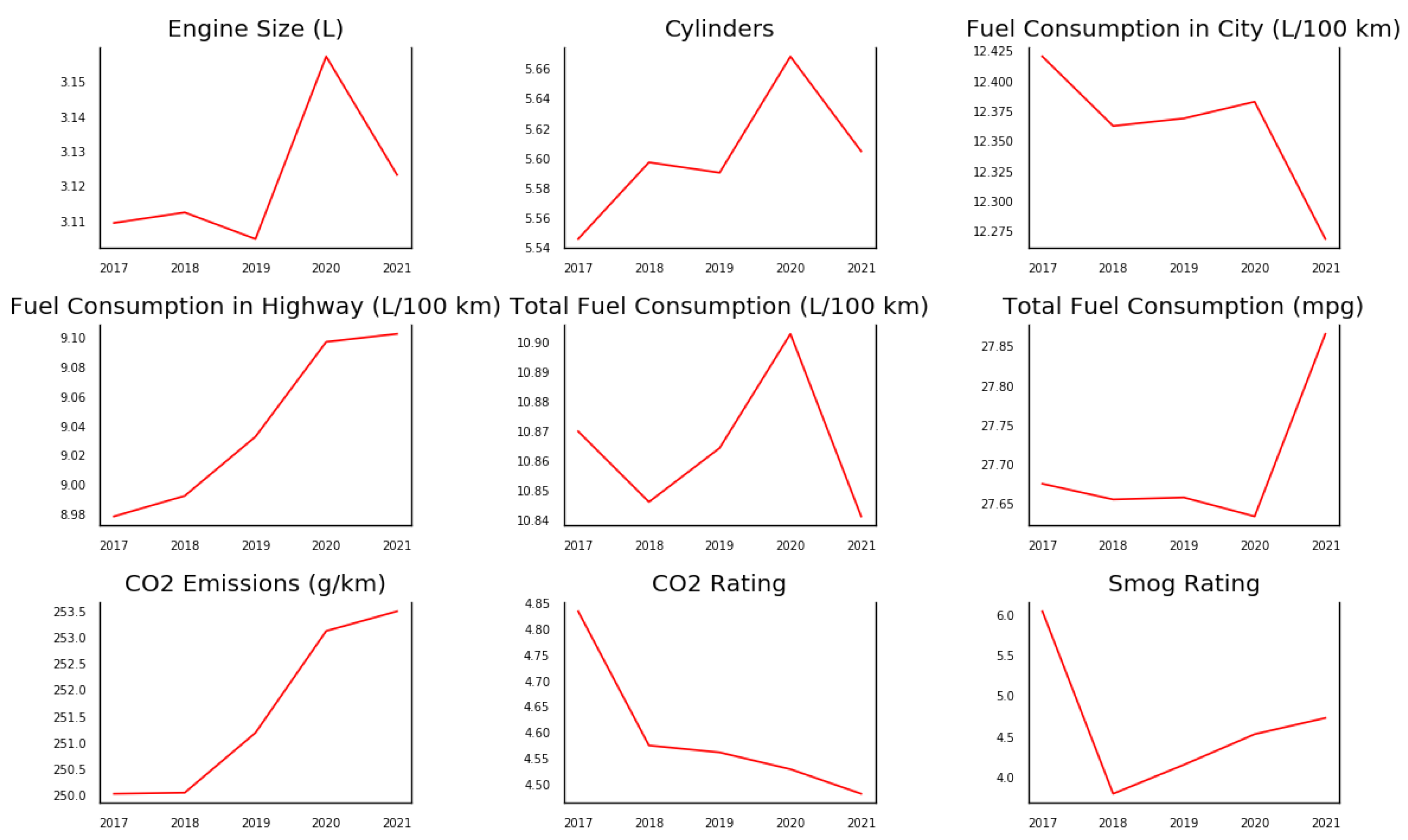
    RQ1.2 How have patterns of fuel consumption and emission of each vehicle type changed throughout the selected period?

  • Level 2: Inferential Statistical Analysis

    -

    RQ2.1 Is there any particular distribution for fuel consumption in the city and the highway of vehicles in Canada?

    -

    RQ2.2 Is there a notable difference in the performance of one specific vehicle (or fuel) type in comparison to the rest of the vehicle types in Canada?

    -

    RQ2.3 How does the brand, model, vehicle class, engine size, cylinder, transmission type, and fuel type correlate with consumption and emissions of various vehicles?

    -

    RQ2.4 What are the relationships between all features to each other of the entire dataset?

  • Level 3: Machine Learning

    -

    RQ3.1 Can fuel consumption and carbon dioxide emission data, and other input metrics be utilized to predict outputs in upcoming years in Canada?

    -

    RQ3.2 Is it possible to build Machine Learning models that use vehicle specifications data to predict their fuel consumption and carbon dioxide emission?

  • Level 4: Deep Learning

    -

    RQ4.1 Is it possible to construct Deep Learning models that use vehicle specifications data to predict their fuel consumption and carbon dioxide emission?

• RO5 To make recommendations and possible regulations and define areas of future research.

To implement and address the listed research objectives, an analytical and predictive study has been conducted on the Government of Canada dataset, containing 4973 light-duty vehicles observed from 2017 to 2021. Using the above-mentioned four levels of data analytics methodology (i.e., Descriptive Statistical Analysis, Inferential Statistical Analysis, Machine Learning, and Deep Learning), the study unravels current trend and comparative analysis of fuel consumption and carbon dioxide emissions from different brands, vehicle models, vehicle class, cylinders, engine size, transmission, fuel type, smog rating, and fuel consumption within a city and on a highway. The research also predicts these features in the upcoming year and builds up a predictive model for fuel consumption and carbon dioxide emission based on relevant car specifications. The results contribute to the quantifying process of energy cost and air pollution caused by transportation, followed by proposing relevant recommendations for both vehicle users and producers. The prediction results from this study discard abrupt factors, such as legislative requirements, unpredictable economic crises, or similar unforeseen interruptions.

2. Literature Review

With the current alarming rate of climate change, due attention ought to be given to the environmental impact of fuel consumption and emissions from light-duty vehicles, particularly passenger cars. Vehicle emissions can be classified into two principal categories: dangerous exhaust emissions for air quality and human health; and emissions that contribute towards climate change. The emission that has the most significant effect on climate change is carbon dioxide (CO₂), which represents the largest proportion of the Green House Gas (GHG) emissions. Notably, road transportation emits about one-fifth of the total emissions of carbon dioxide in the European Union, 75% of which arises from passenger cars [4]. Moreover, the relation between fuel consumption and CO₂ is direct and strong [12]. In the European Union (EU), average fleet emission limits are stated in terms of CO₂ emissions, in grams per kilometer unit. In North America (i.e., the United States (US), and Canada), similar measures have been used, but with limits imposed in terms of fuel economy. Electric vehicles are a critical step in the transportation sector’s decarbonization. However, the International Energy Agency estimates that, by 2030, it is needed to have at least 20% of all road transport vehicles to be powered by electricity in order to keep global warming below 2 °C (approximately 300 million vehicles) [13]. Consequently, light-duty vehicles with low carbon intensity will continue to play a significant role during the transition. Moreover, legislative requirements have been discussed globally; for example, the European Union (EU) has adopted a climate change agenda to reduce GHG emissions by over 55% by 2030 compared to 1990 [14] and become a net-zero GHG emission economy by 2050 [15]. In addition, the Government of Canada has also set the target of reducing its emissions by 40–45% by 2030 and committed to achieving net-zero emissions by 2050 to avert the worst effects of climate change [16]. Therefore, to satisfy those limits in CO₂ and achieve such high targets from legislative requirements, many worldwide researchers have proposed different vehicle emissions and consumption models. The systematic process for this literature review is to specify current approaches that have been used by various researchers, identify which models and methodologies have been used in each approach, before identifying the research gap.

2.1. Vehicle Emissions Estimation Models

A number of vehicle emissions estimation models have been introduced by different researchers in the last decades. Using look-up tables, a micro-scale model called CORSIM is built to estimate emissions based on dynamometer data. To ascertain the total emissions of each link, the CORSIM model applies default emission rates per second to each vehicle that travels on the given link, based on acceleration and speed [17]. EMIT is a model for estimating HC, CO₂, CO, and NOx, which is built from dynamometer data of 344 light-duty vehicles and employs a regression equation with acceleration and speed [18]. At the project or regional level, a United States agency has proposed a model called MOVES in 2010 for the estimations of greenhouse gas emissions: CO, VOCs, PM, and NOx generated from light-duty vehicles [19]. Features such as vehicle mass, total resistance force, velocity, acceleration, and driveline performance have been employed by Rakha and colleagues to build a model for estimating CO₂ emissions using instantaneous vehicle power [20]. A function of acceleration and velocity observed from a dynamometer experiment has been applied to the INTEGRATION model for the estimation of emissions from measured fuel consumption. Additionally, it is further developed for the simulation and optimization of trip-based microscopic traffic [21]. Using more parameters, including 55 parameters, a model named CMEM is proposed by a group of researchers to estimate parameters for a wide range of light-duty vehicles. For dynamometer testing, this model uses emissions per second data of CO, CO₂, NO, and HC, along with physical vehicle features (engine size, vehicle mass, and aerodynamic drag coefficient) and operating features (acceleration and speed) [22]. Another example of using data-intensive parameters is MEASURE, which was invented by the Georgia Institute of Technology. It calculates the emissions of NOx, CO, and VOCs from vehicle operating modes, including acceleration, deceleration, cruise, and idling. However, CO₂ estimation is not included in this model, while it has over 30 features as its inputs [23]. Another well-known framework has been developed by the European Environment Agency (EEA) called COPERT, which became one of the standard methodologies for road transport emission inventories in EEA member countries [24]. It estimates primary air pollutants (CO, NOx, PM, VOC, SO${}_2$, NH${}_3$, heavy metals) and greenhouse gas emissions (CO₂, N${}_2$O, CH${}_4$) using functions of the mean traveling speed throughout a complete driving cycle [25]. However, the framework neglected other characteristics while estimating the emissions of a specific vehicle, such as engine size, cylinders, and engine model.

Furthermore, some recent research authors have applied Machine Learning and Deep Learning methodologies for vehicle emission models. Toth-Nagy and colleagues, for instance, have proposed a model using the Artificial Neural Network to predict emissions of NOx and CO from heavy-duty vehicles. Though the outcome is positive, CO₂ has also not been included, and the model is appropriate for gasoline vehicles [26]. When testing on the real-world driving conditions of 70 diesel vehicles, a group of researchers implemented a machine learning model to make projections of emissions alongside the performance of vehicles. A look-up table, non-linear regression, and Neural Network Multilayer Perceptron models are consequently applied for instantaneous NOx predictions. Despite the model taking inputs of vehicle acceleration and speed, its outputs focus only on NOx estimation, and CO₂ remains excluded [27]. Qing et al. have built a model for estimating vehicle emission rates, including CO, CO₂, HC, and NOx from vehicle idling by using Portable Emission Measurement System. The dataset is collected from actual driving tests; Boosted and Bagged Decision Trees are introduced as a reliable prediction model for vehicle emissions estimation [28]. It can be seen that applying Machine Learning and Deep Learning techniques for predicting carbon dioxide emissions remains limited and needs further development, which is thereby, the principal goal for this study.

2.2. Vehicle Consumption Estimation Models

On the other hand, some researchers have focused on the fuel consumption of vehicles rather than CO₂ emissions, as fuel consumption (and economic costs) seem to be more relevant to consumers in general. The vehicle fuel consumption models are classified into 2 categories: theoretical fuel consumption models and statistical fuel consumption models [29]. The theoretical fuel consumption model concentrates on the operation features of the vehicle, such as output power and engine parameters, while the statistical fuel consumption model converges the statistical attributes from vehicle activity and fuel consumption data, including acceleration and speed [30]. One of the fuel consumption models is based on a novel macroscopic model that considers trip time and intersection distance for prediction [31]. Using the distribution of Vehicle Specific Power, a fuel consumption prediction model is proposed by Qi et al., which comprises a fuel consumption model and traffic condition predictor to provide a real-time prediction. From this, an API is developed for fuel consumption estimation, using on-board diagnostic (OBD) data for verification, with a 20% forecasting error. By collecting driving behavior data from consumers’ smartphones, a prediction model of fuel consumption is developed based on a backpropagation (BP) neural network, random forests, and support vector regression with a relative error of less than 10%. It is also found that the average acceleration and deceleration, acceleration time percentage, deceleration time percentage, and cruising time percentage are major indicators for fuel consumption estimation [10]. Furthermore, Tamer et al. has proposed an approach to estimate fuel consumption by onboard vehicle information system Onboard Diagnoses-II (OBD-II) using Support Vector Machine and Lagrange interpolation. The model successfully provided precise fuel consumption with a square root mean difference of 2.43 [32]. Applying a Machine Learning model, a neural-network-based fuel prediction model is presented by utilizing seven predictors obtained from road grade and vehicle speed. It could optimize fuel usage over the entire fleet, with a peak-to-peak error rate of less than 4% in both city and highway [11].

Furthermore, vehicle emission and consumption can be predicted based on one single model. For example, by using GPS Big Data, an N-Dimensional framework is proposed by a group of researchers for estimating and visualizing fuel consumption and emissions. They stated that analyzing GPS big data generated from vehicles can deliver practical insight on the quantity and distribution of energy use and emissions in real-world driving conditions (acceleration, idle, cruise, and deceleration). This model has claimed effectiveness by a prediction accuracy of 88.6% [8]. Additionally, several statistical models of vehicle emissions and fuel consumption, which are published by Alessandra et al., could be integrated to predict the spatial and temporal distribution of traffic emissions and fuel consumption [18].

Overall, it can be seen from the mentioned studies that numerous researchers have proposed different models for estimating carbon dioxide emissions and fuel consumption using micro-scale methodologies, or Machine Learning and Deep Learning. The common vehicle characteristics for building these models are engine size, vehicle mass, and aerodynamic drag coefficient; and standard operating features used are acceleration and speed. The research trend generally emphasizes improving estimation models, rather than analyzing different vehicle types and brands using vehicle measurements, making it a limited market analysis for users and manufacturers. As a result, for a better knowledge of the vehicle market and its environmental effects, a comparative view of different types of vehicles and their influence on the environment is significant. Based on these metric analyses, recommended prediction models should be built using selective vehicle features. This identified gap provides the basis for the aim and objectives of this research.

3. Methodology

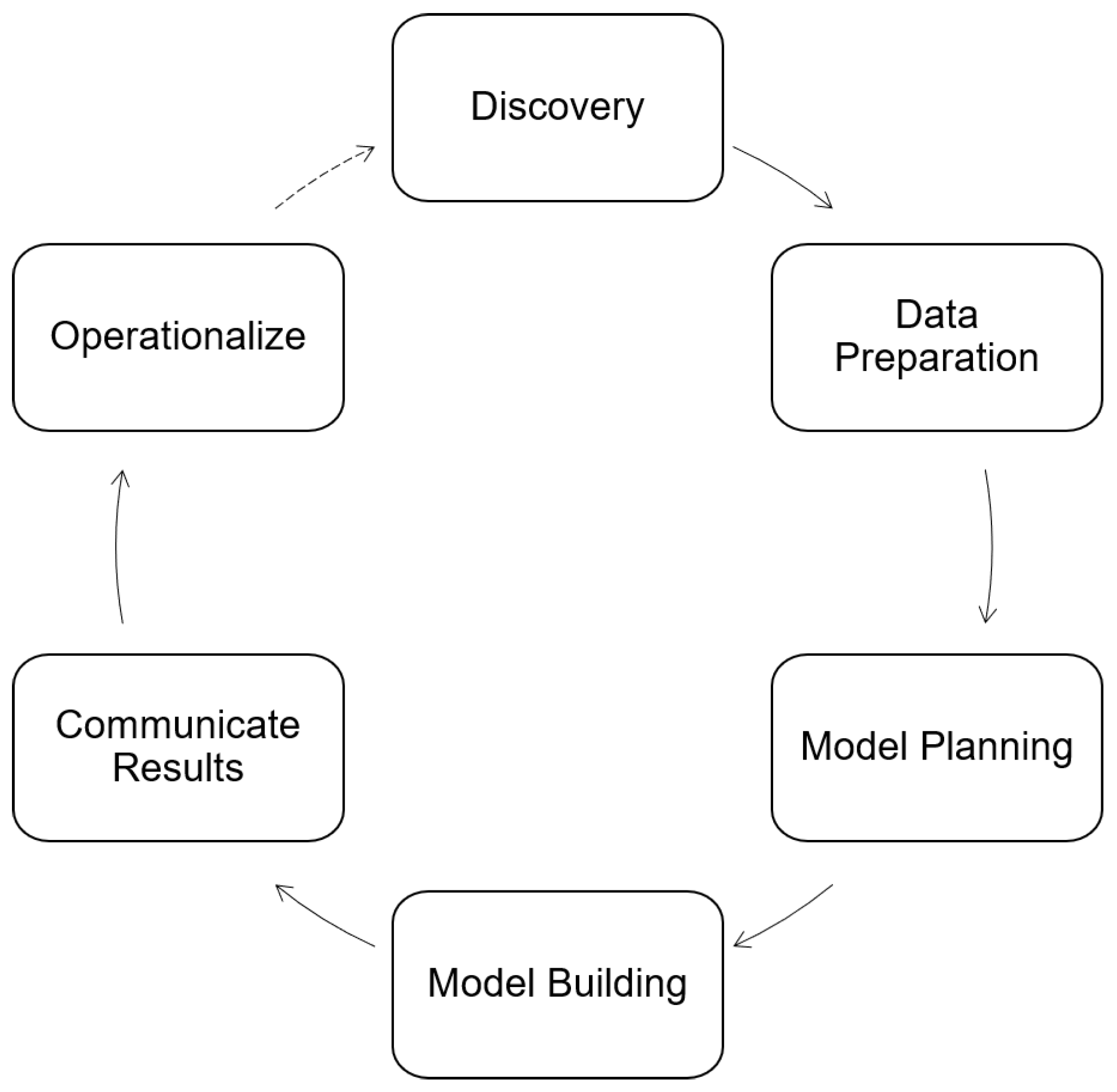
3.1. Macro Methodology

In this study, to conduct an analytical and predictive study for fuel consumption and carbon dioxide emissions of vehicles, the dataset used is collected by the Government of Canada. A data analytics life cycle has been adopted for this research. This life cycle is a standard for Data Science and Big Data Analytics purposes, adopted from EMC Education Services [33], and contains 6 phases, as indicated in Figure 1.

The first stage of this process is discovery, where the problem, context, hypothesis, and objectives that the data are used for are determined. The main goals of this study are to deliver a comparative view of fuel consumption and carbon dioxide emissions from different brands and vehicle models, to make evidence-based recommendations, and to construct a model to predict changes in the future consumption and emission rate. The dataset used in this study is derived from the ‘Fuel consumption rating’ datasets from the Government of Canada, which contains fuel consumption ranks and measured CO₂ emissions for 4974 samples of light-duty vehicles in Canada [34]. The data were originally gathered from vehicle manufacturers, who compile the fuel consumption and CO₂ rating data using standardized, monitored laboratory testing and analytical procedures. Then, a 5-cycle testing process is used by manufacturers to simulate common driving conditions and styles. The approach also includes testing for city and highway driving, as well as driving in cold weather, using air conditioners, and driving at faster speeds with higher acceleration and braking [35]. Note that the CO₂ and smog ratings given in the dataset were generated from the original ratings by manufacturers, not from vehicle testing. Consequently, the collected fuel consumption and CO₂ consumption data from newly produced vehicles are used in this study for data analytics purposes.

In Phase 2—Data Preparation, the dataset has then been processed and compressed into one single spreadsheet. By scoping down the research analysis, data of 4974 light-duty vehicles annually collected from 2017 to 2021 is merged, aggregated, with several renamed categories, including fuel consumption and carbon dioxide emissions from different brands, vehicle models, vehicle class, cylinders, engine size, transmission, fuel type, smog rating, and fuel consumption in a city and on a highway. Next, the dataset has been checked, and there are no issues or missing values. Subsequently, the dataset is cleaned to filter out if any data are not necessary for analysis purposes. For instance, one record is removed from the dataset since it is the only record containing the unique brand named ‘super’ (that can be considered an error record while there is no brand carrying that name), leading to a final 4973 record dataset.

In Phase 3 and 4—Model Planning and Building, the dataset is analyzed and visualized by using four levels of data analytics methodology, including Descriptive Statistical Analysis, Inferential Statistical Analysis, Machine Learning, and Deep Learning methodology. Specific categories of all algorithms are discussed in the next Section 3.2. Finally, in Phases 5 and 6, relevant results on machine learning analytics and predictions are communicated and presented in detail in Section 4 and Section 5 on Results and Discussion. Final reports, briefings, code snippets are also presented in the rest of this paper.

3.2. Micro Methodology

In this paper, the “micro methodology” term refers to the micro-level data analysis methodology. This includes data analysis methods that are critically discussed (supported by embedded citations) by the measurements/approaches/algorithms that will be employed. In particular, four levels of data analytics are applied, as listed below.

3.2.1. Level 1: Descriptive Statistics

This level comprises basic calculations of central tendency (mean, median, mode) and dispersion statistics (standard deviation, variance, range). A list of comparative statistics of fuel consumption and CO₂ emission has been presented for each brand, model, engine size, vehicle class, transmission and cylinder type, and fuel type, giving a comprehensive outlook of emissions and consumption of various vehicle types and brands. The changes of the patterns through the years are also indicated before progressing to time-series changes of the greenest and the least environmental-friendly vehicle brand.

3.2.2. Level 2: Inferential Statistics

The dataset is verified by different types of analytic testing for various purposes.

• t-test: has been conducted to compare the mean fuel consumption in the city and on the highway for the same vehicle;
• ANOVA: compares the means of total fuel consumption and carbon dioxide emissions for each vehicle class and fuel type over time to define whether each fuel type (or vehicle class) is significantly different from the rest;
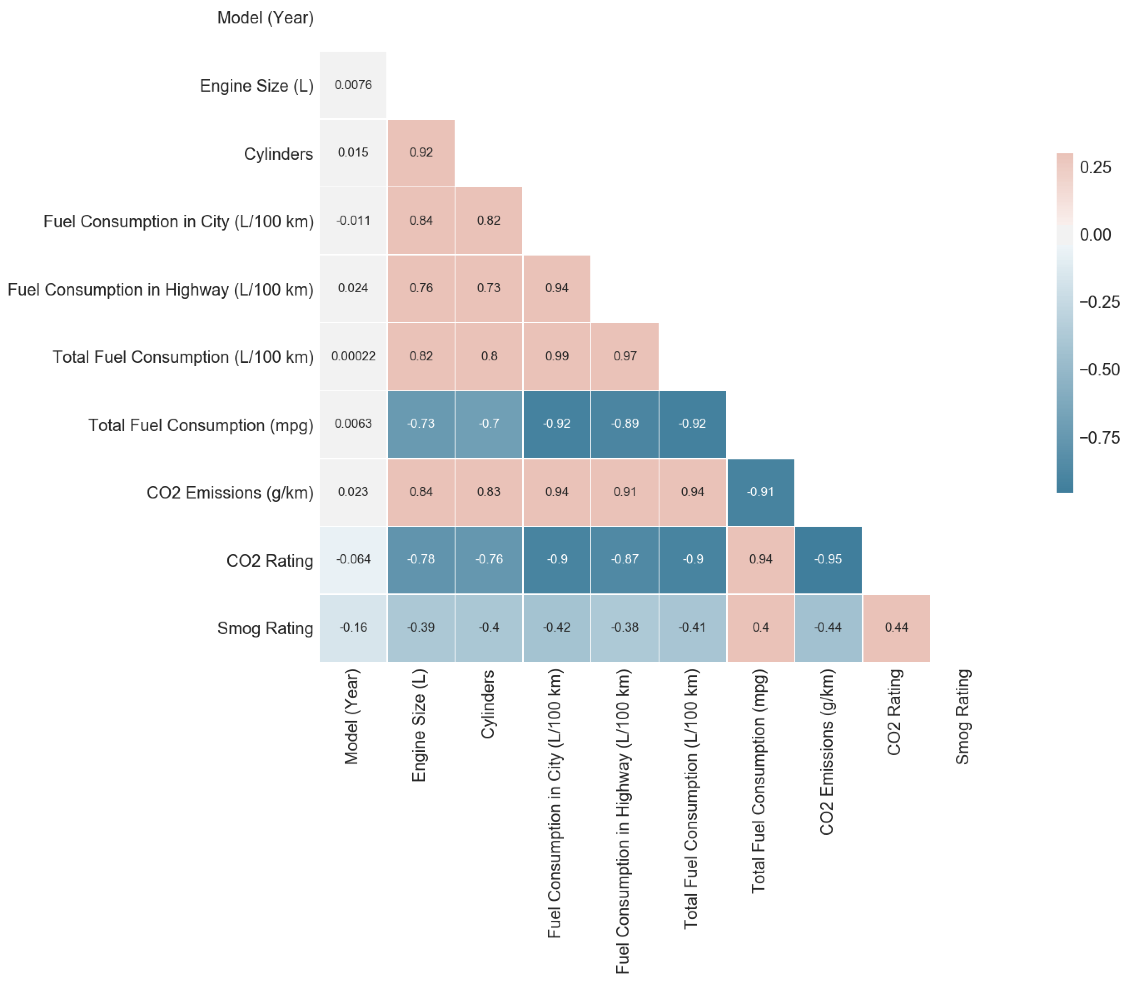
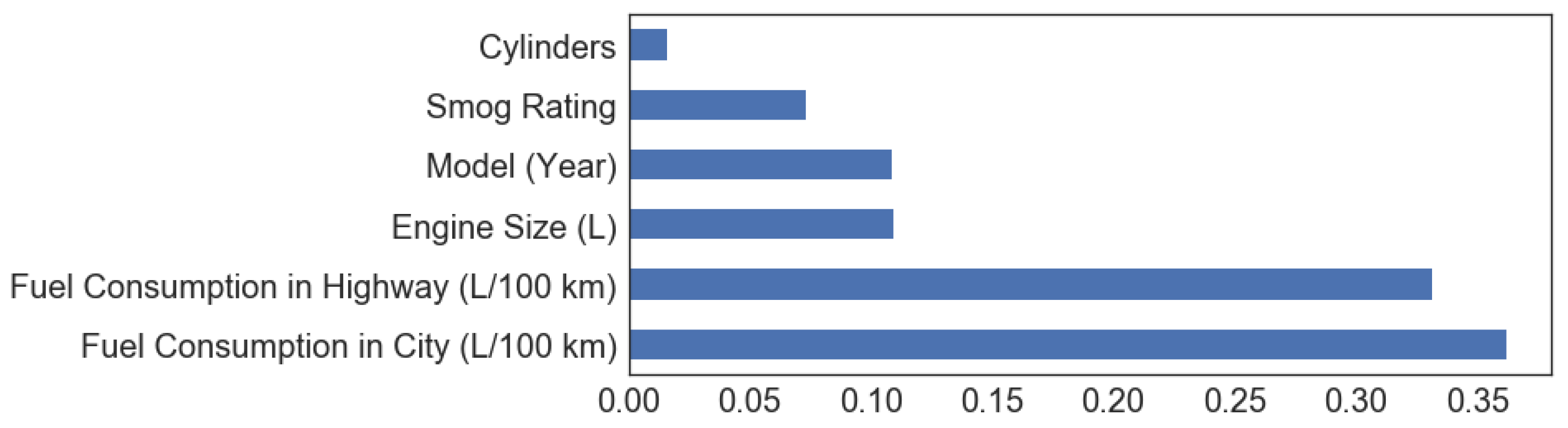
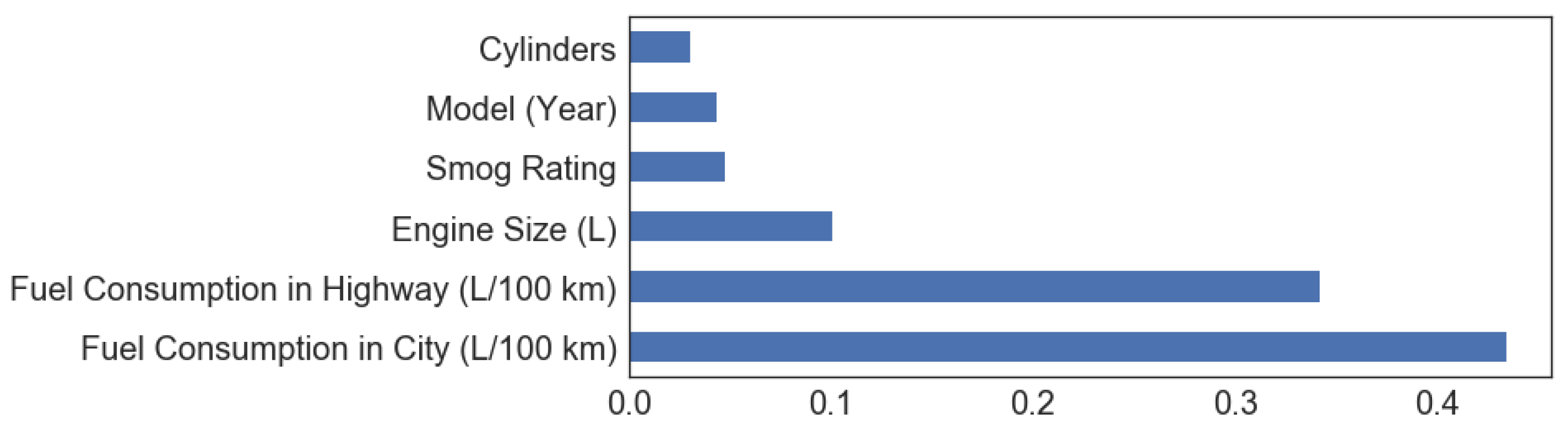
• Correlation: A heat map of correlation coefficients is shown to illustrate the direction and strength of a linear relationship among vehicle features in pairs. Moreover, a comparison of the importance of features for predicting CO₂ Emissions and Total Fuel Consumption has been conducted, which is an important test before advancing to Levels 3 and 4;
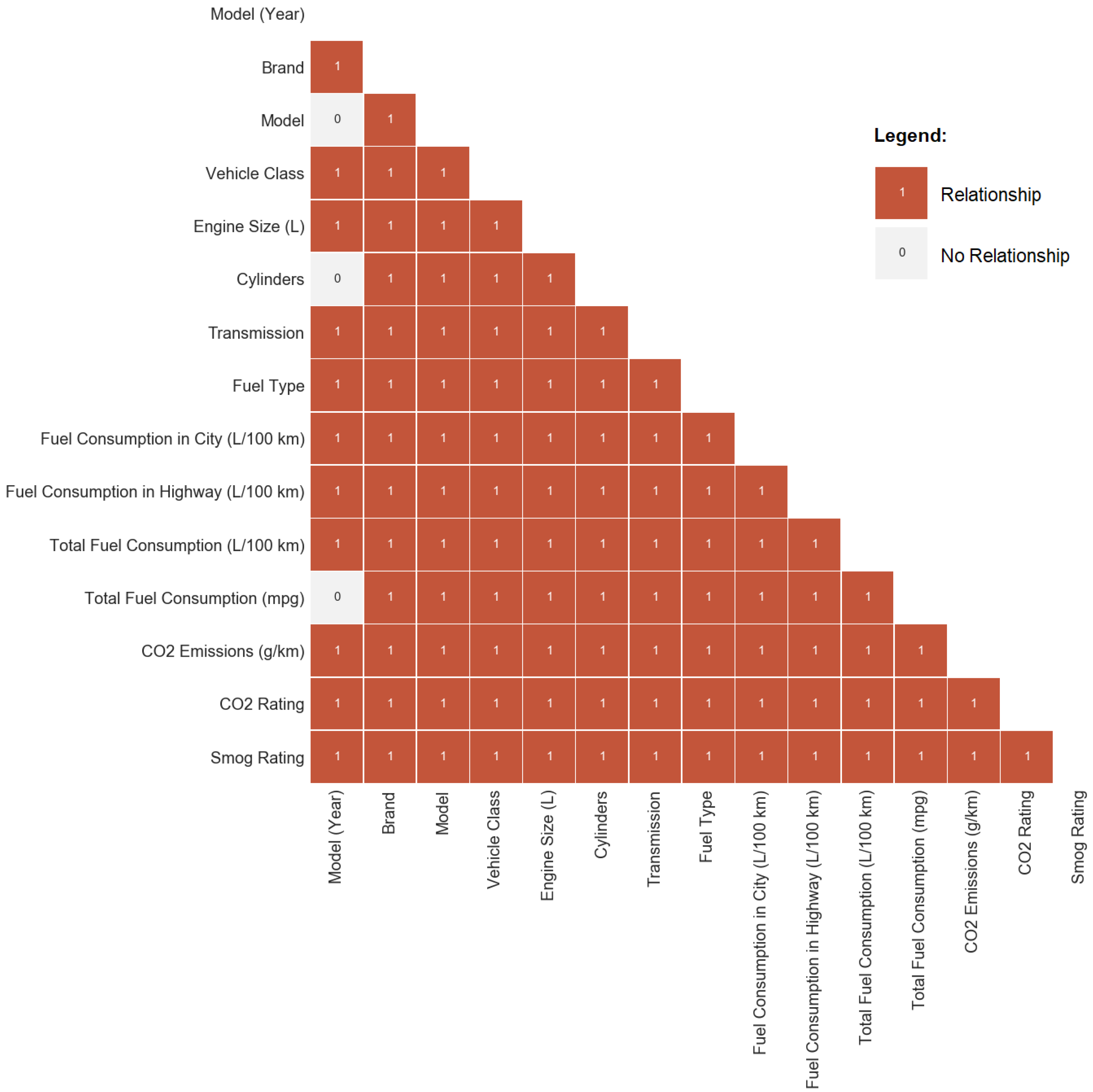
• Chi-Square: Two Chi-Square Goodness of Fit tests have been carried out to investigate whether there is a significant difference between the observed (data in 2021) and expected values (data from 2017 to 2020). Additionally, a chain of Chi-Square of Independence tests have been implemented to define relationships between all features to each other, therefore, presented in a heat map.

3.2.3. Level 3: Machine Learning

In order to answer RQ3.1, input features have been used from the dataset to predict values in upcoming years:

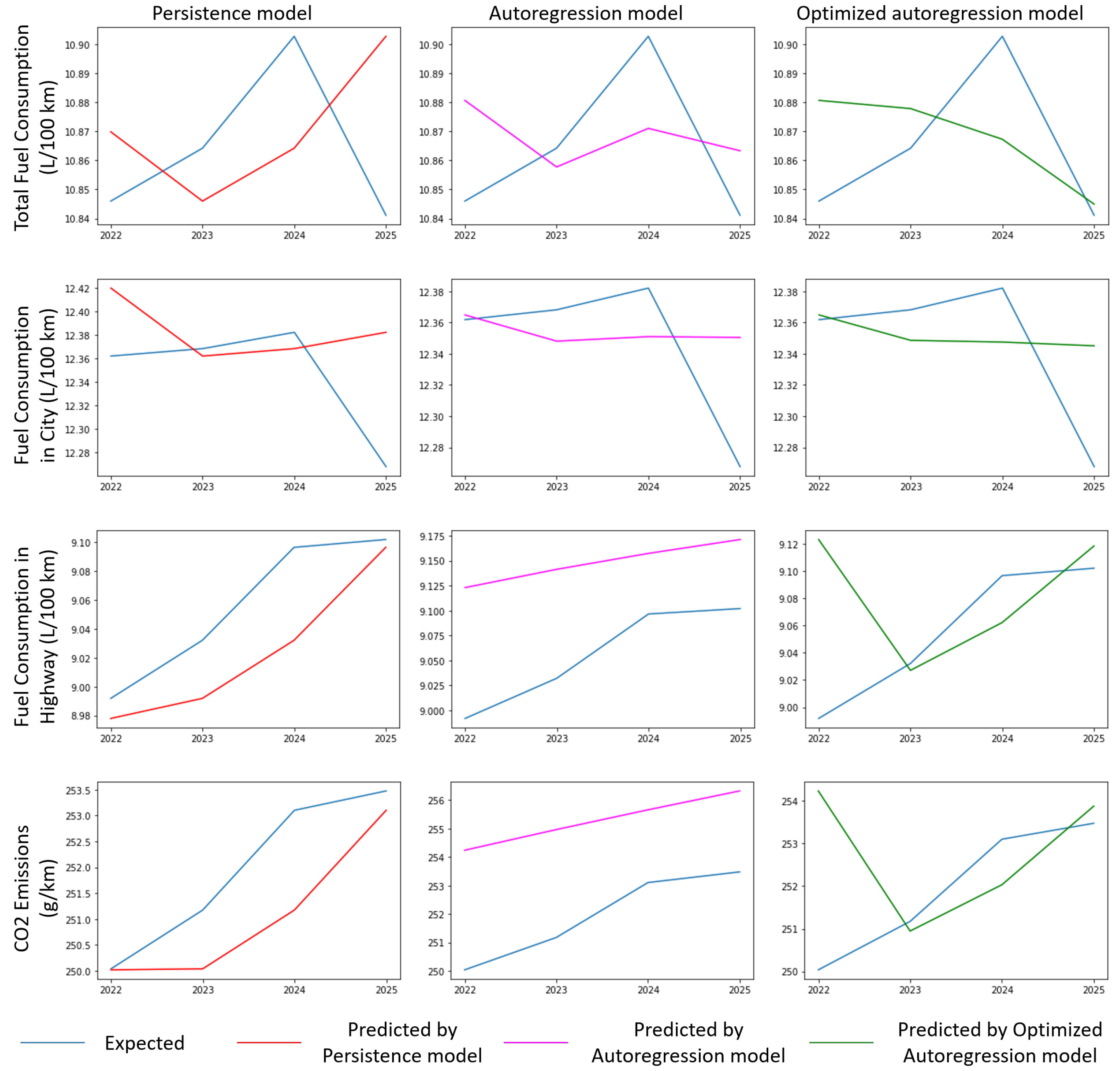
• Time Series Regression: has been used since it can forecast a future response using the historical responses and dynamics transition from related predictors. Different models are applied in this study, including persistence models (using walk forward validation), autoregression models (using autoregression function by statsmodels), and optimized autoregression model (using walk-forward over time steps). These models are evaluated by Root Means Square Error (RMSE) value, which measures the differences between values predicted and the values observed.

To define whether Machine Learning models can use vehicle specifications data to predict their fuel consumption and CO₂ emission (RQ3.2), different models are conducted in this study and classified into two groups: Machine Learning models to predict a variable from a variable; and models to predict a variable from multiple variables.

For building Machine Learning models to estimate a variable from a single variable, data of engine size, number of cylinders, fuel consumption in a city and on a highway have been used to predict total fuel consumption and CO₂ emissions. Moreover, total fuel consumption and CO₂ emission data were used to predict each other. This research uses relevant methodologies to model relationships between those variables, which include:

• Linear Regression: using the sklearn model and the dataset is split into training and testing sets with 80%:20% ratio;
• Univariate Polynomial Regression: using the sklearn model and 5 different degrees (from Degree 1 to Degree 5).

Regarding Machine Learning models used for estimating a variable from multiple variables, groups of data, including group A (model year, engine size, and cylinders) and group B (engine size and cylinders) have been used to predict total fuel consumption and CO₂ emissions. Furthermore, data on fuel consumption in cities and highways were also used to estimate the total fuel consumption of vehicles. The applied models are listed as follows:

• Multiple Linear Regression: using the sklearn model and the dataset is split into training and testing sets with 80%:20% ratio;
• Logarithmic Regression: using the sklearn model with log transformed predictor values and exponential transformed predictor values;
• Exponential Regression: the dataset is split into training and testing sets with 75%:25% ratio;
• Transformation of data: the dataset is split into training and testing sets with 75%:25% ratio;
• Multivariate Polynomial Regression: using the sklearn model and 5 different degrees (from Degree 1 to Degree 5).

These models are chosen because many variables can be used at the same time to examine the statistical significance of each variable and transform them into independent variables. These forms of regression models also support the prediction of the dependent (or target) variables for later analysis [36]. In this paper, the coefficient of decision (R squared) value has been used to evaluate the above-mentioned models. The R squared value is a statistical measurement that examines how differences in one variable can be explained by differences in a second variable. Ranging from 0 to 1, the higher the R squared value, the better the model can be used for prediction.

3.2.4. Level 4: Deep Learning

In addition, Convolutional Neural Network (CNN) is used in this study to predict a variable from multiple variables. Since CNN is normally used for image classification, to use CNN for regression problems, this research uses a one-dimensional convolutional network by reshaping input data. This enables the model to simulate numerical input data using learnable weights and biases [37].

The dataset has two dimensions that are the number of rows and columns (i.e., 4973 rows and 3 columns). Therefore, to reshape the data, a third dimension has been added as the number of the single input row (i.e., it becomes [4973, 3, 1]). Subsequently, the data are split into training and testing sets with an 80:20 ratio. Moreover, Keras is also applied to create a Conv1D class to add a one-dimensional convolutional layer into the model. Flatten and Dense layers are also supplemented and compiled with optimizers. Finally, the model can predict the test data with the trained model. This is evaluated by checking the mean squared error rate (MSE) of the predicted results.

4. Results and Discussion

This section is structured based on the Micro Methodology mentioned in Section 3.2, and divided by four levels of data analytics.

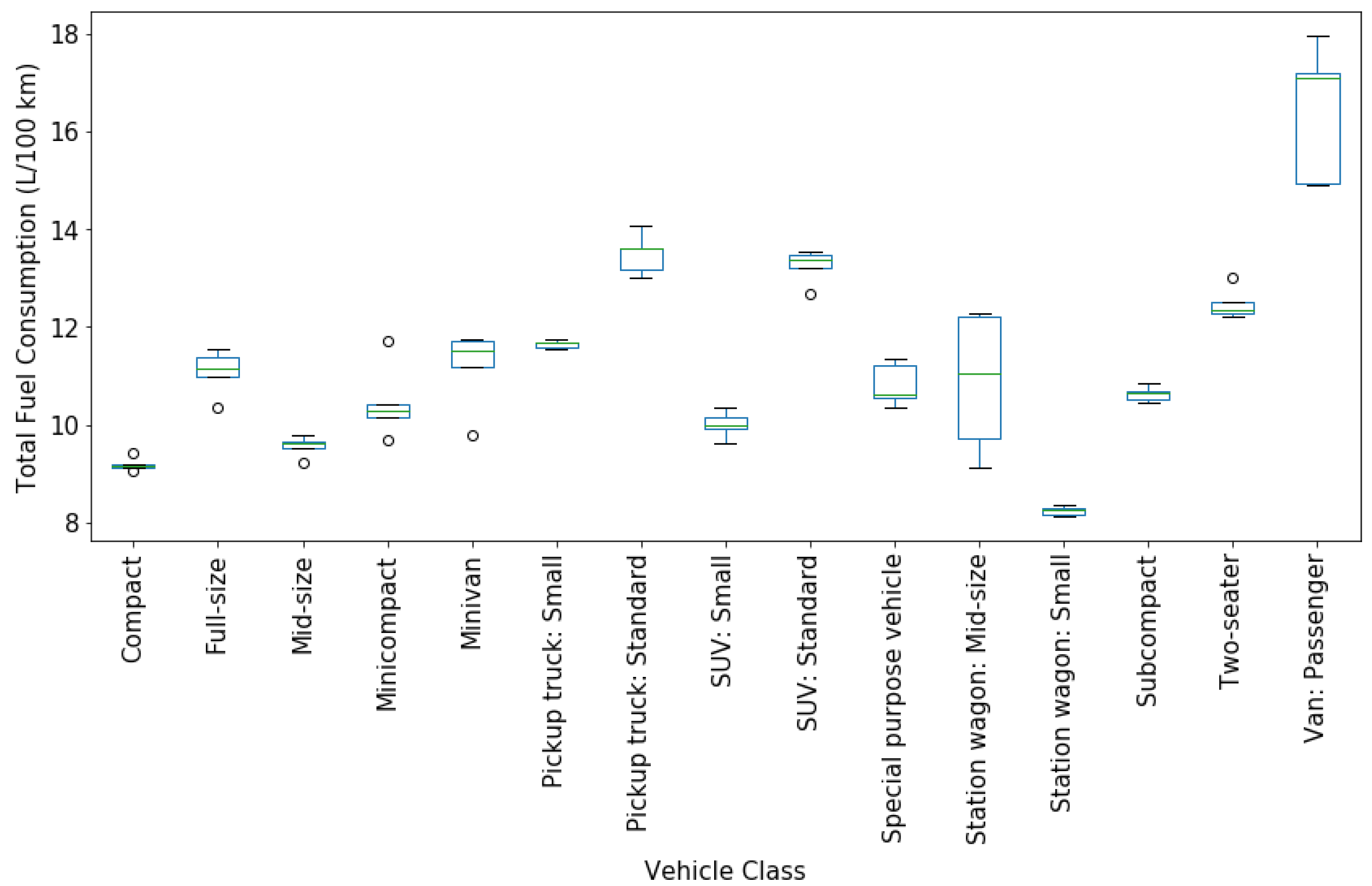
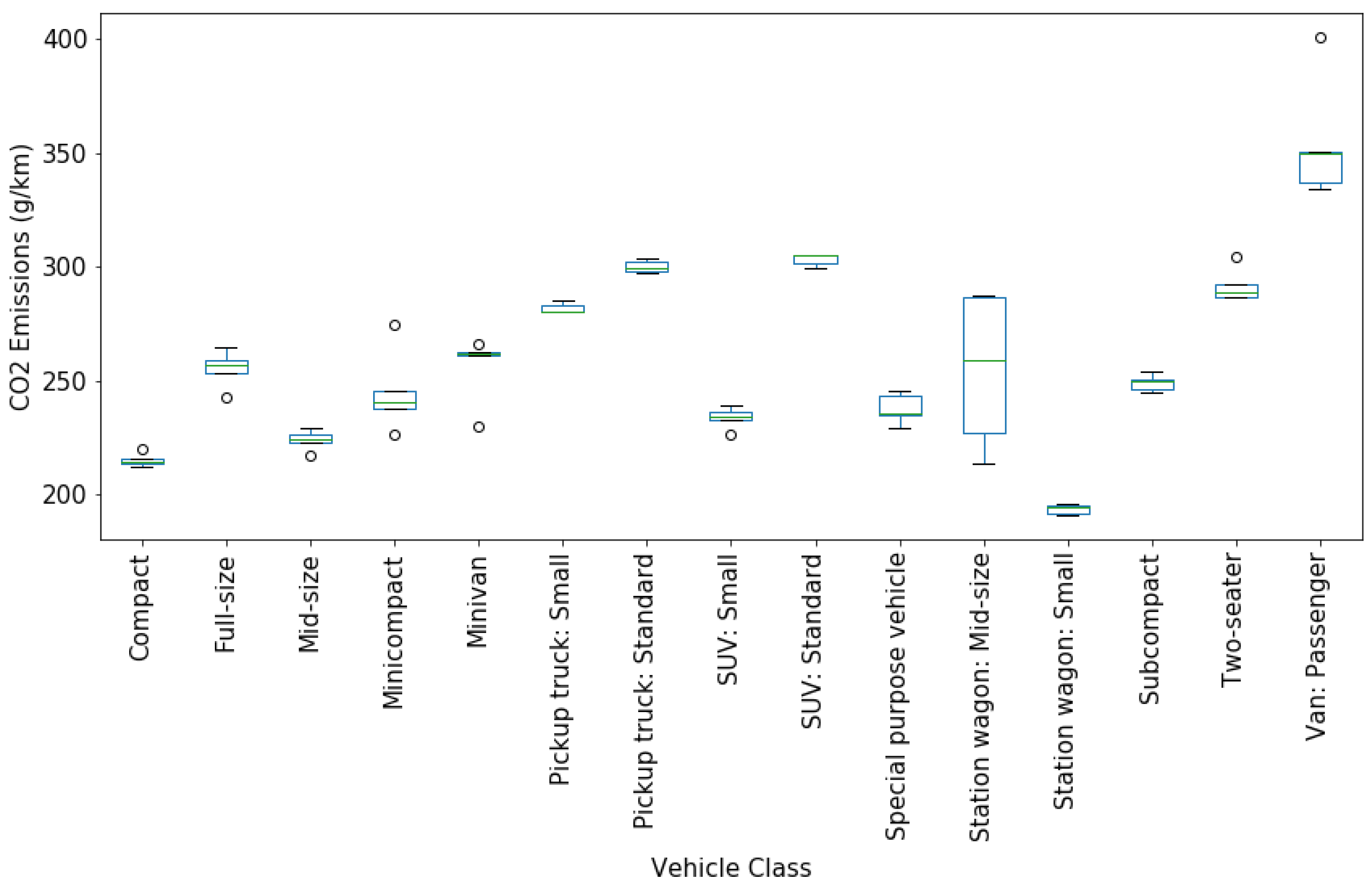
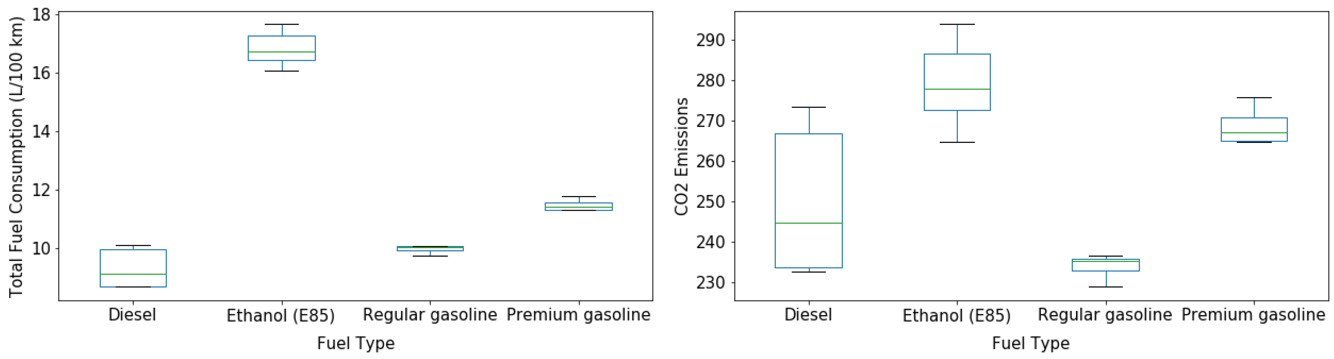
4.1. Level 1: Descriptive Statistics

The general purpose of this Level 1 is to observe 4973 light-duty vehicles from 2017 to 2021 by their fuel consumption and carbon dioxide emissions from different brands, vehicle models, vehicle class, cylinders, engine size, transmission, fuel type, smog rating, and fuel consumption in a city and on a highway. Recall that the CO₂ and smog ratings in the dataset were calculated using manufacturer ratings rather than vehicle testing, and were ranked from worst (1) to best (10) with no unit.

Firstly, in order to address RQ1.1 (How do light-duty vehicles compare in terms of fuel consumption and carbon dioxide emission?), descriptive statistics for all numerical columns in the dataset have been conducted to provide an evaluation of the data distribution. The purpose of descriptive statistics is to provide a statistical understanding of the dataset quality [36]. It can be seen from

Table 1. Descriptive statistics of numerical columns of the dataset.

Feature	Mean	Standard Deviation	Min	Max	Variance
Engine Size (L)	3.120	1.345	1.0	8.4	1.809
Cylinders	5.599	1.882	3.0	16.0	3.542
Fuel Consumption in City (L/100 km)	12.363	3.355	4.0	30.3	11.256
Fuel Consumption in Highway (L/100 km)	9.036	2.086	3.9	20.9	4.351
Total Fuel Consumption (L/100 km)	10.865	2.747	4.0	26.1	7.548
CO2 Emissions (g/km)	251.436	58.851	94.0	608.0	363.459
CO2 Rating	4.601	1.6588	1.0	10.0	2.752
Smog Rating	4.635	1.807	1.0	8.0	3.265

that the average total fuel consumption is 10.86 L/100 km, of which 57.77% (12.36 L/100 km) from the city and 42.22% from the highway (9.04 L/100 km). Additionally, it is clear from the statistics that the average CO₂ emissions of all vehicles are 251.44 g/km, with a standard deviation of 58.85 g/km. Ranking from worst (1) to best (10), the average CO₂ rating is 4.60, and the average smog rating is 4.63. Moreover, dispersion statistics of standard deviation and variance also indicate that the size of the distribution of values expected is reliable enough for prediction. Regarding the fuel consumption and carbon dioxide emission of different brands, their average data are indicated in

Table 2. Average data of different vehicle brands.

Brand	Engine Size (L)	Cylinders	Total Fuel Consumption (L/100 km)	CO2 Emissions (g/km)	CO2 Rating	Smog Rating
Honda	2.01	4.35	8.03	187.58	6.65	4.65
Mitsubishi	1.88	3.85	8.32	193.63	6.29	5.38
Mazda	2.30	4.00	8.36	195.92	6.23	5.80
Hyundai	2.05	4.18	8.45	199.42	6.17	5.14
FIAT	1.51	4.00	8.47	198.37	6.11	4.69
MINI	1.81	3.62	8.61	201.56	5.86	6.13
Kia	2.25	4.43	8.80	207.89	5.94	5.09
Volkswagen	2.00	4.17	9.02	210.97	5.67	6.45
Toyota	2.83	4.92	9.17	214.58	5.87	5.48
Subaru	2.28	4.13	9.31	217.63	5.42	4.34
Volvo	2.00	4.00	9.54	222.70	5.14	5.44
Acura	2.96	5.21	9.72	227.62	5.06	4.40
Buick	2.34	4.57	9.74	228.64	5.05	5.30
Alfa Romeo	2.20	4.55	9.78	229.97	5.00	3.09
Nissan	2.92	5.10	9.90	232.59	5.17	4.99
Lexus	3.44	5.86	10.14	237.21	4.90	5.40
Audi	2.78	5.54	10.60	247.67	4.59	4.68
Cadillac	3.15	5.38	10.86	255.29	4.32	5.18
Jaguar	3.03	5.73	10.87	256.47	4.38	6.21
Jeep	2.93	5.05	10.90	254.74	4.36	4.67
Infiniti	3.27	5.78	10.97	257.67	4.25	4.13
BMW	3.19	6.15	11.10	260.01	4.31	4.50
Porsche	3.09	5.80	11.17	260.98	4.19	2.84
Land Rover	3.05	5.64	11.35	272.23	3.91	5.07
Lincoln	2.74	5.17	11.37	266.92	4.17	5.19
Chrysler	3.79	6.14	11.52	252.12	4.40	4.65
Mercedes-Benz	3.36	6.51	11.60	271.25	3.99	4.66
Chevrolet	3.73	5.98	11.77	268.15	4.19	4.47
Genesis	3.55	6.06	11.86	279.48	3.76	4.24
Ford	3.11	5.53	11.96	264.23	4.16	4.56
Ram	4.32	6.70	12.79	294.59	3.45	3.77
GMC	4.27	6.54	12.96	291.36	3.51	4.38
Dodge	4.97	7.06	13.06	295.52	3.35	2.99
Maserati	3.35	6.65	13.55	317.29	2.77	2.04
Aston Martin	4.98	10.46	13.63	320.50	2.96	3.58
Bentley	5.39	9.94	15.48	361.67	2.00	3.30
Rolls-Royce	6.65	12.00	16.72	390.95	1.03	3.62
Lamborghini	5.64	10.67	17.65	410.79	1.54	1.77
Bugatti	8.00	16.00	22.98	538.83	1.00	1.00

.

In this dataset, the number of vehicles from Ford accounts for the highest with 436 vehicles, and the lowest amount is from Bugatti with 6 vehicles. After the descriptive statistical analysis, a bar chart is created, as presented in Figure 2, to demonstrate the average fuel consumption of different brands. It reveals that Honda consumes fuel the least (8.03 L/100 km), while Bugatti has the highest fuel consumption (22.98 L/100 km). Moreover, from Figure 3 and Figure 4, Honda seems to be the greenest brand as it emits the least CO₂ (187.58 g/km) and attains the highest CO₂ rating (6.65), whereas Bugatti continues to perform poorly in its environmental-friendliness with the highest CO₂ emissions (538.83 g/km) and the worst CO₂ rating (1.00).

Considering smog, Figure 5 proves that Volkswagen emits smog the least (6.45), and Bugatti seems to be the worst brand in terms of smog (1.00), fuel consumption, and CO₂ emissions.

Regarding fuel consumption and CO₂ emissions of different models,

Table 3. CO₂ emissions (g/km) and total fuel consumption (L/100 km) of each model.

Model	Total Fuel Consumption (L/100 km)	CO2 Emissions (g/km)
IONIQ BLUE	4.08	95.60
IONIQ	4.28	101.40
PRIUS	4.48	105.40
...
AVENTADOR COUPE SVJ	22.40	520.00
DIVO	23.00	537.00
CHIRON PUR SPORT	26.10	608.00

explains that the IONIQ BLUE model consumes and emits the least, and in contrast, the CHIRON PUR SPORT model consumes and emits the most.

Similarly, when considering fuel consumption and CO₂ emissions,

Table 4. CO₂ emissions (g/km) and total fuel consumption (L/100 km) of each vehicle class.

Vehicle Class	Total Fuel Consumption (L/100 km)	CO2 Emissions (g/km)
Station wagon: Small	8.25	193.85
Compact	9.22	215.69
Mid-size	9.55	223.49
SUV: Small	10.01	233.65
Minicompact	10.35	242.16
Subcompact	10.64	248.95
Special purpose vehicle	10.77	236.90
Station wagon: Mid-size	10.86	254.41
Full-size	11.16	256.36
Minivan	11.30	257.98
Pickup truck: Small	11.66	281.61
Two-seater	12.45	291.33
SUV: Standard	13.25	303.00
Pickup truck: Standard	13.48	300.05
Van: Passenger	16.98	362.63

,

Table 5. CO₂ emissions (g/km) and total fuel consumption (L/100 km) of each engine size.

Engine Size (L)	Total Fuel Consumption (L/100 km)	CO2 Emissions (g/km)
1.2	6.66	155.11
1.6	7.38	176.19
1.8	7.61	178.19
...
6.8	18.62	434.40
6.5	20.62	478.25
8.0	22.98	538.83

,

Table 6. CO₂ emissions (g/km) and total fuel consumption (L/100 km) of each cylinder.

Cylinders	Total Fuel Consumption (L/100 km)	CO2 Emissions (g/km)
3	7.78	181.78
4	8.85	207.12
5	10.37	242.43
6	11.49	265.59
8	14.00	318.05
10	15.09	353.19
12	16.60	388.24
16	22.98	538.83

,

Table 7. CO₂ emissions (g/km) and total fuel consumption (L/100 km) of each transmission type.

Transmission	Total Fuel Consumption (L/100 km)	CO2 Emissions (g/km)
AV1	6.82	161.50
AV	7.13	167.14
AM6	7.35	171.33
AV10	7.75	181.29
AV6	8.02	187.15
M5	8.23	191.55
AV7	8.29	194.37
A4	9.05	212.50
AV8	9.05	211.49
M6	9.95	233.09
AS6	10.39	237.62
AS9	10.57	247.82
A9	10.87	253.26
AM9	11.00	259.75
AS8	11.13	260.67
AM8	11.18	261.78
M7	11.32	264.73
AM7	11.33	265.04
AS7	12.08	282.10
AS10	12.31	277.96
A8	12.35	286.17
A10	12.60	304.13
A5	12.95	295.37
AS5	13.11	305.64
A6	13.15	288.23
A7	13.26	310.85

and

Table 8. CO₂ emissions (g/km) and total fuel consumption (L/100 km) of each fuel type.

Fuel Type	Total Fuel Consumption (L/100 km)	CO2 Emissions (g/km)
D (Diesel)	9.32	250.52
X (Regular gasoline)	9.98	234.05
Z (Premium gasoline)	11.47	268.38
E (Ethanol E85)	16.62	275.43

showcase that Station wagon (Small) class, Engine Size 1.2L, 3 Cylinders, Transmission Type AV1, and Fuel Type D (Diesel) consume fuel and emit CO₂ the least. Conversely, Van (Passenger) class, Engine Size 8.0, 16 Cylinders, Transmission Type A6, and Fuel Type E (Ethanol E85) seem to be the most consumers and emitters. However, since the Volkswagen emissions scandal emerged, the negative image of diesel has intensified. The actual NO and PM emissions of diesel vehicles, according to recent researchers, are significantly greater than those reported. Because of carcinogenic compounds, diesel particle emissions are also a possible health danger [38]. Therefore, the conclusion that Ethanol E85 emits the most among other fuel types remains the scope of the data in this research.

Secondly, to answer RQ1.2 (How have patterns of consumption and emission of each vehicle type changed throughout the selected period?), descriptive statistics have been conducted for total CO₂ emissions and fuel consumption through the period of 2017 to 2021 in

Table 9. CO₂ emissions (g/km) and total fuel consumption (L/100 km) over time.

Model (Year)	Total Fuel Consumption (L/100 km)	CO2 Emissions (g/km)
2017	10.87	250.02
2018	10.85	250.04
2019	10.86	251.17
2020	10.90	253.10
2021	10.84	253.48

in general.

It can be seen from Table 9 that the total fuel consumption gradually increases from 2017 to 2020, before a significant drop in 2021. However, the peak in 2020 does not exist in the CO₂ emissions, and the value steadily rises over the entire period.

From

Table 10. Average feature data over time.

Model (Year)	2017	2018	2019	2020	2021
Engine Size (L)	3.11	3.11	3.10	3.16	3.12
Cylinders	5.54	5.60	5.59	5.67	5.60
Fuel Consumption in City (L/100 km)	12.42	12.36	12.37	12.38	12.27
Fuel Consumption in Highway (L/100 km)	8.98	8.99	9.03	9.10	9.10
Total Fuel Consumption (L/100 km)	10.87	10.85	10.86	10.90	10.84
Total Fuel Consumption (mpg)	27.67	27.65	27.66	27.63	27.86
CO2 Emissions (g/km)	250.02	250.04	251.17	253.10	253.48
CO2 Rating	4.83	4.57	4.56	4.53	4.48
Smog Rating	6.04	3.78	4.14	4.52	4.72

, it can be seen a similar pattern of gradually increasing from 2017 to 2020 before significantly dropping in the data of engine size, cylinders, fuel consumption in the city, and the total. The highway fuel consumption and in total (mpg) and CO₂ emission observe a continuous rise over the years. That could explain a gradual decrease in CO₂ rating during the period. Finally, smog rating dramatically is reduced in 2018, before continuously growing until 2021.

In this research, it is evident that Honda is the greenest brand, and it is essential to analyze its pattern of consumption and emission through the years. From Figure 6, in 2018, Honda seems to have optimized fuel consumption and carbon dioxide emissions of their products. Although the data in 2019 and 2020 show a slight increase, it dramatically drops again in 2021.

Given the same analysis on the brand that has demonstrated to possess the least environmental awareness, Bugatti has never considered optimizing their products’ consumption and emission, proven by the significant growth in total fuel consumption and CO₂ emission shown in Figure 7.

Considering the fuel consumption of each fuel type during the years, it can be seen from Figure 8 that Fuel Type E (Ethanol E85) and Z (Premium gasoline) always consume more than Fuel Type X (Regular gasoline) and D (Diesel). Over the period, Fuel Type D (Diesel), E (Ethanol E85), and Z (Premium gasoline) all have increased their consumption, whereas Fuel Type X (Regular gasoline) has a slight decrease, thus having the least fuel usage in 2021.

4.2. Level 2: Inferential Statistics

4.2.1. t-Test

To address RQ2.1 (Is there any particular distribution for fuel consumption in the city and the highway of vehicles in Canada?), a two-tailed t-test has been conducted to compare the means of fuel consumption in the city and on the highway for the same vehicle, with the following configurations.

• Null Hypothesis (H0): mean of fuel consumption in the city = mean of fuel consumption on a highway;
• Alternative Hypothesis (Ha): mean of fuel consumption in a city ≠ mean of fuel consumption in highway;
• Chosen confidence level: 99%, which means $\alpha$ = 0.01.

After the test, the result showed that:

• Statistic = 149.8128 (t-value);
• p-value = 0.0.

It is clear that:

$$p-value=0.0<\alpha /2=0.005.$$

(1)

Therefore, the null hypothesis can be rejected. This means the mean of fuel consumption in a city and on a highway for the same individual has a significant difference.

4.2.2. ANOVA

To answer RQ2.2 (Is there a notable difference in the performance of one specific fuel type (or vehicle type) in comparison to the rest of the vehicle types in Canada?), a one-way ANOVA one-tailed test was implemented to compare the means of each vehicle class in terms of total fuel consumption, using the following assumptions.

• The samples are not dependent;
• Each sample comes from a population that is normally distributed;
• The group population standard deviations are all equal (homoscedasticity).

Firstly, the means of total fuel consumption for each class through the years is calculated based on the descriptive statistics method, as shown in Figure 9.

The following configurations have been set out.

• Null Hypothesis (H0): means of each vehicle class are the same;
• Alternative Hypothesis (Ha): At least one of the means for each class is not equal to the other;
• Chosen Confidence Level: 99%, which means $\alpha$ = 0.01

After the test, the result showed that:

$$p-\mathrm{value}=2.3552\times {10}^{-27}<\alpha =0.01.$$

(2)

Therefore, the null hypothesis can be rejected, meaning that at least one mean of total fuel consumption for each vehicle class is significantly different from the rest.

Similarly, using the same assumptions, hypothesis, and confidence level, one-way ANOVA one-tailed tests have been conducted in CO₂ emissions and fuel consumption of each vehicle class and fuel type (Figure 10 and Figure 11, respectively) of each fuel type, and each result is presented as the following.

$$p-\mathrm{value}=6.81894\times {10}^{-27}<\alpha =0.01.$$

(3)

Consequently, the null hypothesis can be rejected, meaning that at least one mean of CO₂ emissions for each vehicle class is significantly different from the rest.

Total fuel consumption of each fuel type over time:

$$p-\mathrm{value}=1.3362\times {10}^{-13}<\alpha =0.01.$$

(4)

Therefore, the null hypothesis can be rejected, meaning that at least one mean of total fuel consumption for each fuel type is significantly different from the rest.

Emissions of each fuel type over time:

$$p-\mathrm{value}=5.5127\times {10}^{-05}<\alpha =0.01.$$

(5)

From that comparison, the null hypothesis can be rejected, meaning that at least one mean of CO₂ emissions for each fuel type is significantly different from the rest.

4.2.3. Correlation

To define the strength of the relationship among two features in the dataset and address RQ2.3 (How the brand, model, vehicle class, cylinder, engine size, transmission type, and fuel type correlate with emissions and consumption of various vehicles?), a correlation algorithm has been introduced to generate correlation coefficients. The most commonly used algorithm of this type in statistics is Pearson correlation, which estimates the direction and strength of a linear relationship among two variables [39]. In this study, the objective of this statistic is to define which parameter has the strongest correlation with the total fuel consumption and CO₂ emission. To achieve this, Pearson’s correlation coefficients have been applied and computed between all features through all vehicles and presented in a correlation heat map shown in Figure 12.

From the heat map in Figure 12, all the correlation coefficients have been calculated, showing the correlation between corresponding parameters on the left and the corresponding parameters at the bottom. The higher the correlation coefficient, the warmer color was presented.

Moreover, Figure 13 and Figure 14 below reveal the importance of all features on estimating total fuel consumption and CO₂ emissions by using bar charts.

It is seen from Figure 13 and Figure 14 that besides the fuel consumption features in the highway and the city (the two most important features), engine size gives the highest correlation for estimating total fuel consumption, whereas cylinders, year, and smog rating are nearly half as important, compared to engine size. For estimating carbon dioxide emission, engine size, year, and smog rating are important features. This finding contributes as an influential factor in building Machine Learning and Deep Learning models presented in Levels 3 and 4.

4.2.4. Chi-Square

Chi-Square is a non-parametric test, which is divided into two different types: Chi-Square Goodness of Fit and Chi-Square of Independence. The purpose of Chi-Square Goodness of Fit is to compare the observed and expected values from one categorical variable. Meanwhile, Chi-Square of Independence defines whether there is an association among categorical variables, meaning that the variables are related or independent, known as the Chi-Square Test of Association [40].

To implement the Chi-Square Goodness of Fit test, the dataset is split into the period of 2017 to 2020, used for testing the predictions of 2021 whether there is a significant difference between the observed and expected values. First, the Chi-Square Goodness of Fit Test is applied to compare the Total Fuel Consumption by Vehicle Class between expected (from 2017 to 2020) and observed (2021) using a confidence level of 98% ($\alpha$ = 0.02), and the results attained are discussed below.

• Chi-Square value: 0.5317;
• p-value: 0.4659.

It can be seen that:

$$p-\mathrm{value}=0.47>\alpha =0.02.$$

(6)

Therefore, the null hypothesis can be accepted, meaning that there is no significant difference between the observed and expected values.

A similar Chi-Square Goodness of Fit Test is conducted for comparing Total Fuel Consumption by Fuel Type in expected (from 2017 to 2020) and observed (2021) with the following outputs.

• The Chi-Square value is: 6.3380;
• p-value: 0.0118.

$$p-\mathrm{value}=0.012<\alpha =0.02.$$

(7)

Therefore, the null hypothesis can be rejected, meaning that there is a significant difference between the observed and expected values.

Next, to address RQ2.4 (What are the relationships between all features to each other of the entire dataset?), the Chi-Square of Independence Test was conducted to ascertain whether there is a relationship between fuel type and CO₂ rating and the results are the following.

• The Chi-Square value is: 765.5951;
• The p-value is: 6.6296 × 10${}^{-144}$;
• The degree of freedom is: 27.

It is perceived that

$$p-\mathrm{value}=6.63\times {10}^{-144}<\alpha =0.02.$$

(8)

With the chosen confidence level of 98%, the null hypothesis is rejected, and there is a relationship between fuel type and CO₂ rating.

A chain of similar Chi-Square of Independence tests have also been implemented to define relationships amongst all features and are presented in a correlation heat map shown in Figure 15. In the heat map, all the correlation coefficients have been calculated and indicated as 1, if there is a relationship between corresponding parameters on the left and the corresponding parameters at the bottom, and indicated as 0 if there is no relationship among them. It reveals that there is some form of relationship amongst almost all features except that there is no relationship between year and model, cylinders, and total fuel consumption (mpg). Through this test, it is concluded that all the features from the chosen dataset can be used for prediction models proposed in Level 3 and 4, and year can be used as a time index for the estimation.

4.3. Level 3: Machine Learning

4.3.1. Time Series Regression

This subsection aims to answer RQ3.1 (Can fuel consumption and carbon dioxide emission data and other input metrics be utilized to predict outputs in upcoming years in Canada?). To determine which Machine Learning models can be used for predicting fuel consumption and carbon dioxide emission, different experiments were conducted, as presented below.

Firstly, all the input features from the dataset are used to calculate their mean values over time, as shown in Figure 16.

Secondly, using the correlation results from Section 4.2.3, this study builds the following models to predict the fuel consumption (in city, highway, and total) and CO₂ emissions of an average vehicle in Canada in the four upcoming years.

• Persistence models (using walk-forward validation);
• Autoregression models (using autoregression function by statsmodels);
• Optimized autoregression model (using walk-forward over time steps).

The prediction results of these models are presented in Figure 17 and

Table 11. Root Means Square Error (RMSE) of different regression models.

Metric	Persistence Model	Autoregression Model	Optimized Autoregression Model
Total Fuel Consumption	0.002	0.026	0.026
Fuel Consumption in City	0.004	0.045	0.044
Fuel Consumption in Highway	0.002	0.097	0.068
CO2 Emission	1.287	3.412	2.178

.

It can be observed from Table 11 that the autoregression model always has the highest RMSE. The optimized autoregression model has lower values, while the persistence model has the lowest values. The persistence model predicts that total fuel consumption and CO₂ emission will increase in the next four years. However, fuel consumption in the city is projected to decline, while the data in highways are expected to grow firmly.

The rest of the following Machine Learning models have been constructed to answer RQ3.2 (Is it possible to build Machine Learning models that use vehicle specifications data to predict their fuel consumption and carbon dioxide emission?).

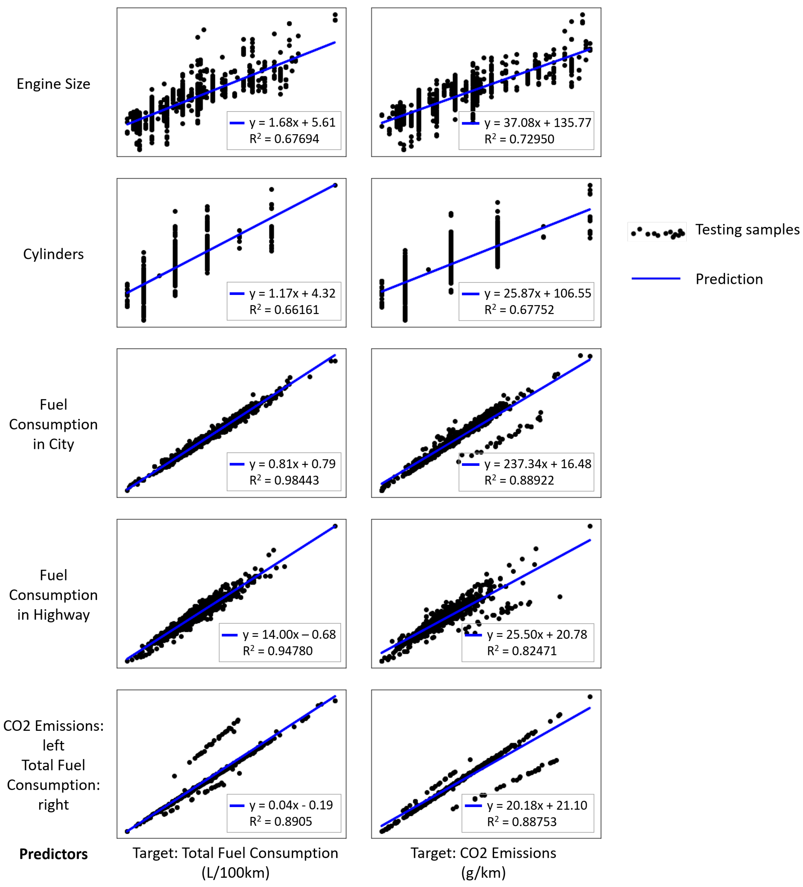
4.3.2. Linear Regression and Univariate Polynomial Regression

These methodologies have been applied to build models that predict total CO₂ emissions and fuel consumption of vehicles from a single input (engine size, or the number of cylinders, etc.), and the result is presented in

Table 12. Coefficient of determination (R squared) values of Linear Regression and Univariate Polynomial Regression models.

Predictor	Target	Linear Regression	Univariate Polynomial Regression
			Degree 1	Degree 2	Degree 3	Degree 4	Degree 5
Engine Size	Total	0.67694	0.67670	0.68466	0.68611	0.69022	0.69038
Cylinders	Fuel Con	0.66161	0.64166	0.65108	0.65165	0.65595	0.65596
Fuel Consumption in City	sumption	0.98443	0.98606	0.98606	0.98624	0.98626	0.98626
Fuel Consumption in Highway	(L/100	0.94780	0.94710	0.94778	0.94783	0.94790	0.94794
CO2 Emissions	km)	0.89053	0.88828	0.88851	0.88859	0.88894	0.88894
Engine Size	CO2	0.72950	0.70852	0.71446	0.72162	0.72480	0.72552
Cylinders	Emis-	0.67752	0.69280	0.69839	0.69962	0.70195	0.70195
Fuel Consumption in City	sions	0.88922	0.88654	0.89650	0.89724	0.90846	0.90886
Fuel Consumption in Highway	(g/km)	0.82471	0.82107	0.84835	0.84839	0.85369	0.85448
Total Fuel Consumption		0.88753	0.88828	0.90243	0.90289	0.91193	0.91215

and Figure 18.

The coefficient of determination is ranged from 1 to 10, from worst to perfect prediction.

It can be seen from Table 12 that the Univariate Polynomial Regression Degree 5 model achieves the highest coefficient of determination (R squared) in 7 out of 10 scenarios. Being insignificantly different from it, the Linear Regression almost attains the same R squared value and at the same time, obtains the highest in 3 out of 10 scenarios.

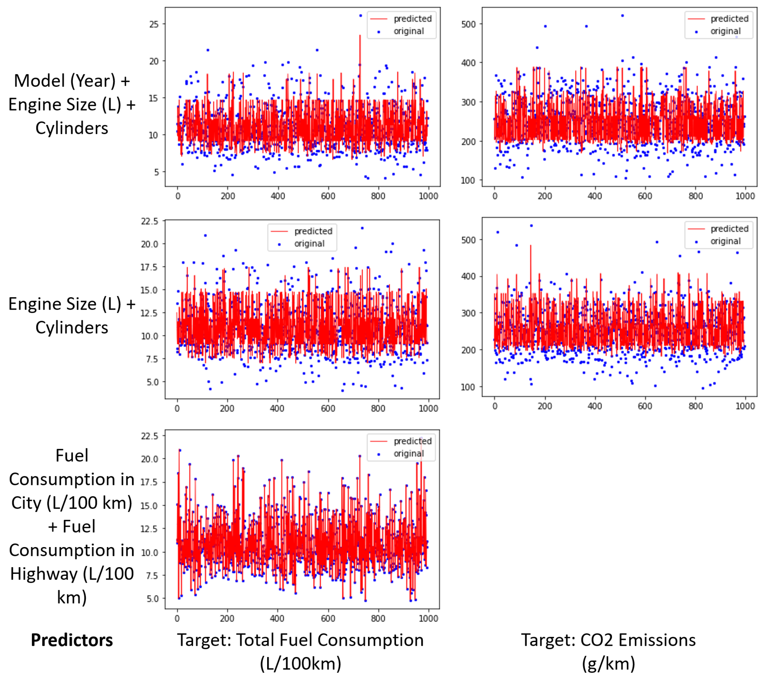
4.3.3. Multiple Linear Regression, Logarithmic Regression, Multivariate Polynomial Regression, Transformation of Data, and Exponential Regression

These models are selected to estimate total CO₂ emissions and fuel consumption of vehicles from multiple inputs, and the result is presented in

Table 13. Coefficient of determination (R squared) values of Multiple Linear Regression, Logarithmic Regression, Multivariate Polynomial Regression, Transformation of data, and Exponential Regression models.

Predictor	Target	Multiple Linear Regression	Logarithmic Regression		Univariate Polynomial Regression
			Log Transformation	Exponential Transformation	Degree 1	Degree 2	Degree 3	Degree 4	Degree 5
Model (Year) + Engine Size (L) + Cylinders	Total Fuel Consumption (L/100 km)	0.68184	0.61418	−0.31802	0.68658	0.69331	0.69174	0.70389	0.67582
Engine Size (L) + Cylinders		0.71549	0.62154	−0.31802	0.68728	0.69041	0.69018	0.70343	0.71083
Fuel Consumption in City (L/100 km) + Fuel Consumption in Highway (L/100 km)		0.99968	0.55998	−0.31802	0.99968	0.99968	0.99968	0.99968	0.99968
Model (Year) + Engine Size (L) + Cylinders	CO2 Emissions (g/km)	0.74119	0.49410	−0.04007	0.71355	0.71902	0.72576	0.72994	0.70450
Engine Size (L) + Cylinders		0.73955	0.42943	−0.04007	0.71247	0.71506	0.72388	0.72922	0.73300

.

Table 13 shows that in 3 out of 5 cases, the Multiple Linear Regression model has the largest coefficient of decision (R squared). Despite being insignificantly different from it, the Linear Regression comes close to attaining the same R squared value and also achieves the best score in 2 out of 5 scenarios (at Degree 2 and 5). On the other hand, the Logarithmic Regression with Log Transformation model receives lower determination scores in all scenarios. Notably, the Logarithmic Regression with Exponential Transformation model generates negative R squared values in all cases, implying that the goodness of fit level is worse than fitting the curve of the model.

In this subsection, different Machine Learning models are applied to use vehicle specifications data for fuel consumption and carbon dioxide emission estimation. It is recognized that Linear Regression, Multiple Linear Regression, Univariate Polynomial Regression, and Multivariate Polynomial Regression are very potential in this field, which answered the research question RQ3.2.

4.4. Level 4: Deep Learning

Convolutional Neural Network

To address RQ4.1, a Convolutional Neural Network (CNN) [41,42] has been employed in this study to estimate the total CO₂ emissions and fuel consumption of vehicles from multiple inputs. CNN is a form of deep neural network that is often used to explore visual imagery [37,43]. The deep learning model has been built using Google Collab and results are presented in Figure 19 and

Table 14. Coefficient of determination (R squared) values of Convolutional Neural Network.

Predictor	Target	Convolutional Neural Network
Model (Year) + Engine Size (L) + Cylinders	Total Fuel Consumption (L/100 km)	0.70061
Engine Size (L) + Cylinders		0.69482
Fuel Consumption in City (L/100 km) + Fuel Consumption in Highway (L/100 km)		0.99964
Model (Year) + Engine Size (L) + Cylinders	CO2 Emissions (g/km)	0.68912
Engine Size (L) + Cylinders		0.71746

.

It can be seen from Table 14 that the CNN model always delivers stable and high coefficient of determination values in all scenarios. Compared with Table 13, while the CNN model is yet to reach the highest R squared score, in any case, the model is likely to attain it with stable predictions. Moreover, Figure 19 demonstrates that the CNN model could predict with high accuracy.

5. Recommendations

Through a series of rigorous data analyses, the study has showcased the current trend and comparative analysis of fuel consumption and carbon dioxide emissions from different brands and vehicle features.

A list of recommendations for customers who currently wish to buy new vehicles is as follows:

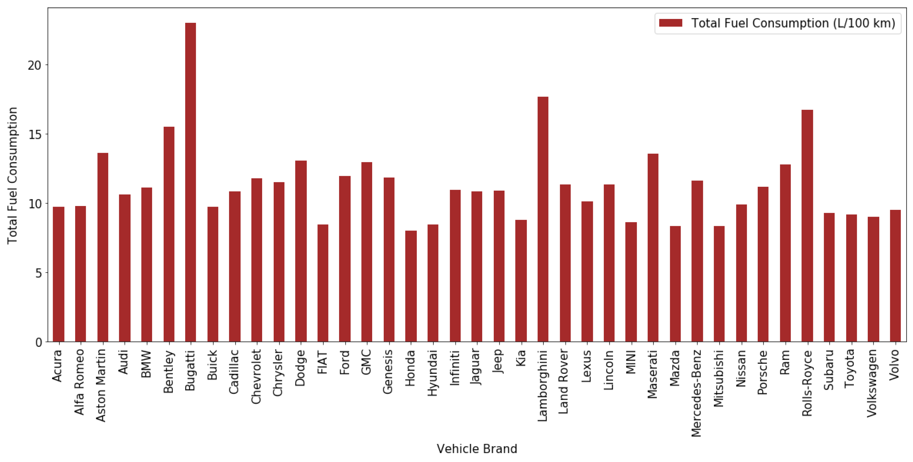
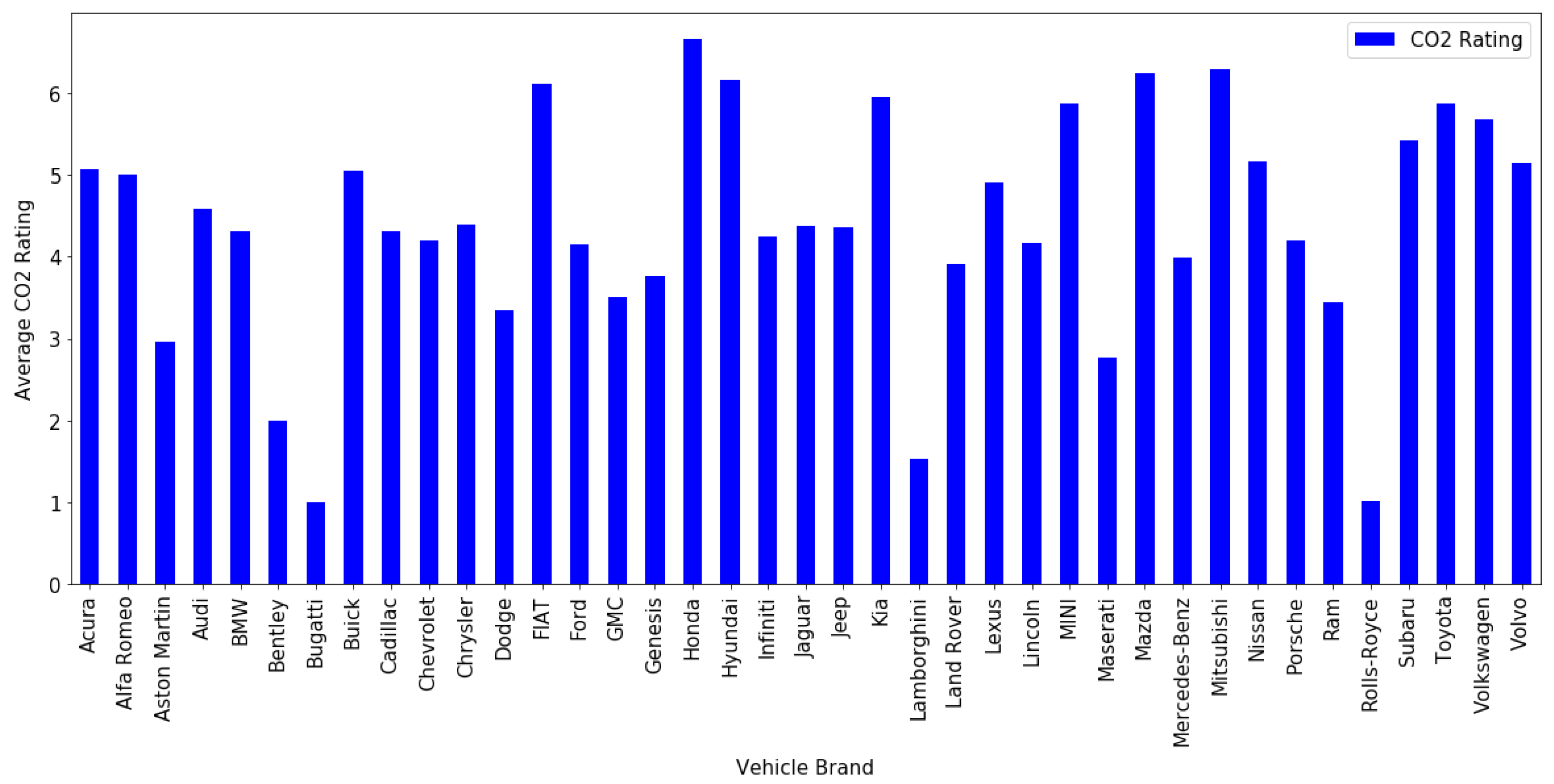
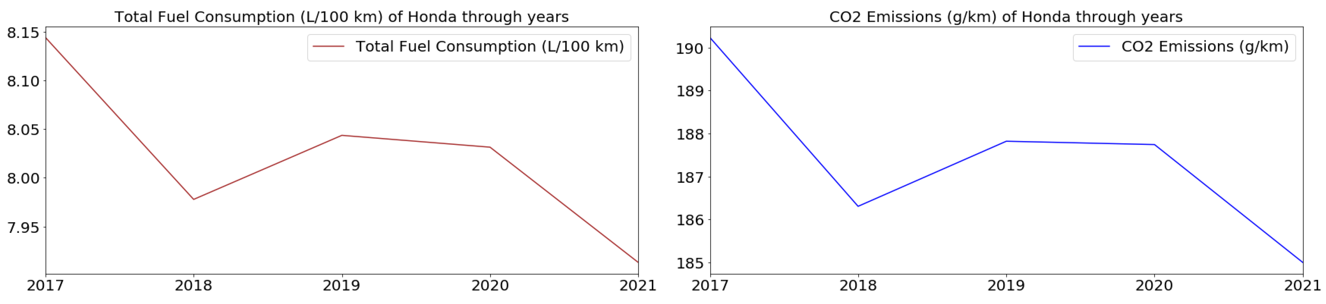
• Fuel-saver and environmental-friendly brands: Honda, Mitsubishi, Mazda, FIAT, Hyundai, MINI, Kia, and Volkswagen;
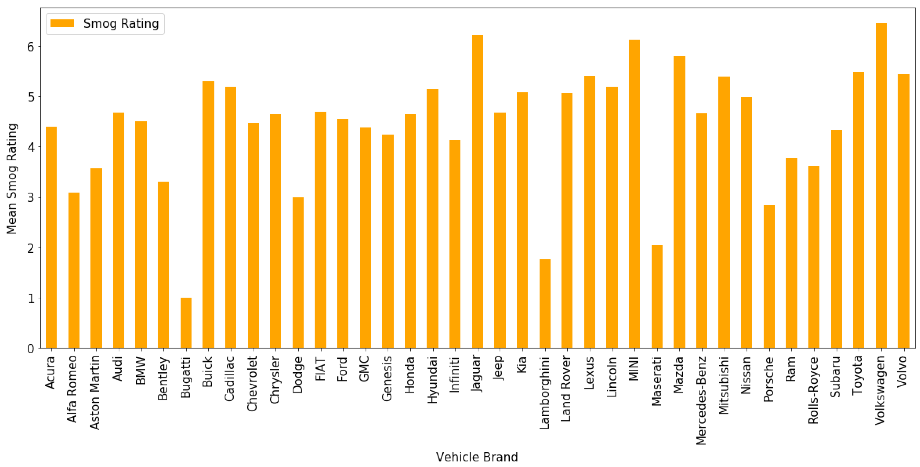
• Least smog-emitter brands: Volkswagen, Jaguar, MINI, Mazda, Toyota, Volvo, and Lexus.

Conversely, customers who are environmental friendly ought to reconsider the following brands:

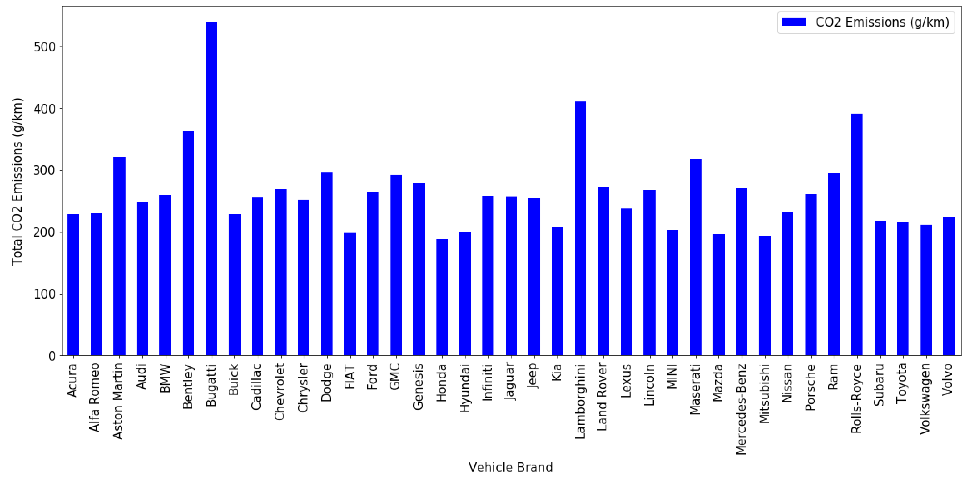
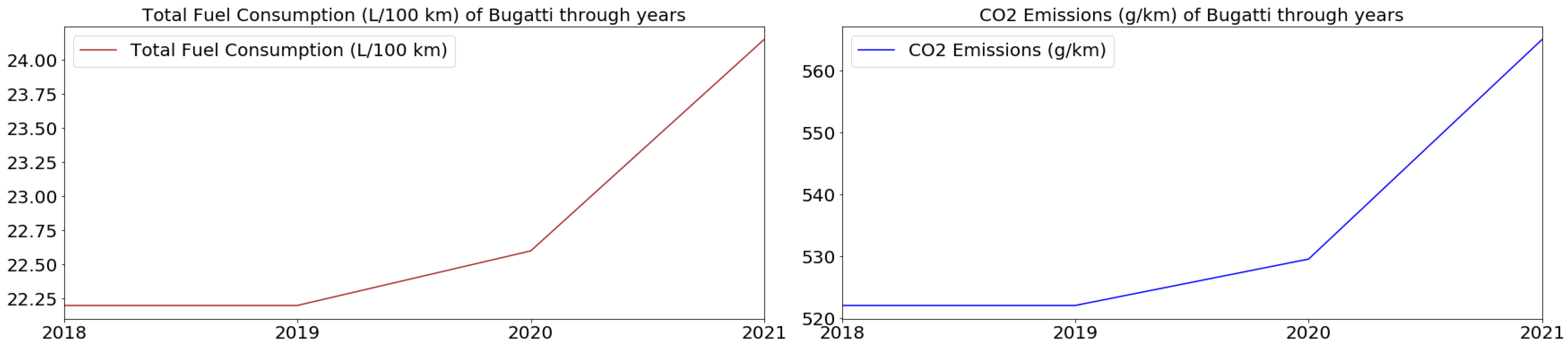
• Brands with high fuel consumption and CO₂ emissions: Bugatti, Lamborghini, Rolls-Royce, Bentley, Aston Martin, Maserati, and Dodge;
• Brands with high smog emissions: Bugatti, Lamborghini, Maserati, Porsche, Dodge, Alfa Romeo, and Bentley.

Recommendations for both vehicle producers and customers who strive to be green in their products are as follows:

• Engine models: IONIQ Blue, IONIQ, Prius, Corolla Hybrid, And Niro FE;
• Suggested Vehicle Classes: Station wagon (Small), Compact, Mid-size, and SUV (Small);
• For engine size and cylinder, the smaller, the better for fuel consumption and CO₂ emissions;
• Suggested transmission type: AV1, AV, AM6, AV10, and AV6;
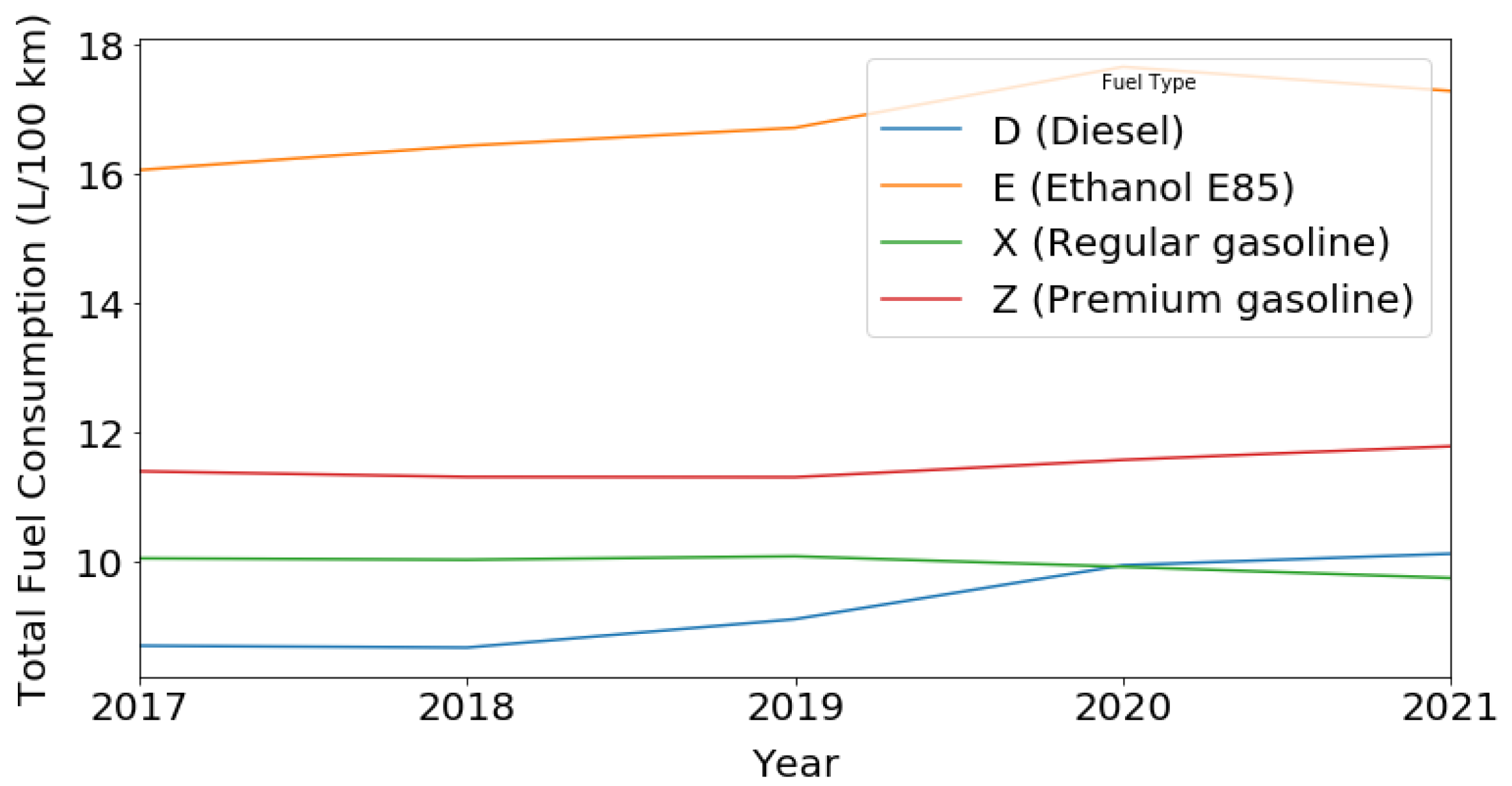
• About Fuel type, it is recommended to use fuel types D (Diesel) and X (Regular gasoline).

Due reconsideration has to be made regarding the following products in terms of their negative environmental impacts:

• Engine models: Chiron PUR Sport, Divo, Aventador Coupe S, Aventador Coupe SVJ, and Aventador Roadster S;
• Vehicle Classes that have high fuel consumption and CO₂ emission: Van (Passenger), Pickup truck: Standard, and SUV: Standard;
• For engine size, the bigger, the worse for fuel consumption and CO₂ emissions;
• Not recommended transmission type: A7, AS5, A10, A5, A6, and A8;
• About Fuel type, it is not recommended to use fuel types Z (Premium gasoline) and E (Ethanol E85).

From the findings of our in-depth statistics and analysis of different Machine Learning and Deep Learning model, there are several evidence-based recommendations. First, it is possible to use engine size and the number of cylinders to estimate CO₂ emissions and fuel consumption of future vehicle designs, with a relatively high determination coefficient, around 70%. Moreover, fuel consumption and CO₂ emission data can be used to predict each other, with every high accuracy in most cases, up to 91.22%. Secondly, different Machine Learning models, including Linear Regression, Multiple Linear Regression, Univariate Polynomial Regression, and Multivariate Polynomial Regression have potential to predict the CO₂ emission and fuel consumption of light-duty vehicles. However, it is suggested to apply Convolutional Neural Network for the prediction, which is proven to predict stably with relatively high accuracy of around 70%. Prediction results from the Machine Learning and Deep Learning models in this paper can be used as an index and a reference for relevant predictors, that can be used for different stakeholders in the upcoming actions. Moreover, the models can be applied to other air pollutants of the vehicle exhausts, including CO, NOx, SO2, PM, etc.

6. Conclusions and Future Work

In this research, an observational and predictive analysis has been performed using data from the Government of Canada, which includes 4973 light-duty vehicles observed between 2017 and 2021, to provide a comparative view of various brands and vehicle types in terms of fuel consumption and CO₂ emissions before making applicable recommendations. Despite significant efforts that have been developed in the past [10,19,27], this research analyzes different vehicle types and brands using vehicle measurements, providing a deeper understanding of the vehicle market and its environmental effects. The proposed vehicle features and recommended prediction models in this study can be further used as a reference for vehicle manufactures and users to make relevant actions for reducing their environmental impacts.

By using descriptive and inferential statistics methodologies, it is observed that the average total fuel consumption of light-duty vehicles is 10.86 L/100 km, and the average CO₂ emission is 251.44 g/km. Different brands and vehicle features have been included in a rigorous, as well as comprehensive, analysis. Based on the findings, relevant recommendations have been made. Over the study period, some vehicle brands have been working towards optimizing their products with environmental awareness (such as Honda), while some are doing conversely (including Bugatti).

Moreover, different machine learning and deep learning models have been built throughout this study for fuel consumption and CO₂ emission prediction. Firstly, this study reveals that the Persistence model has outperformed the autoregression and optimized autoregression models for predictions from one input variable with vector autoregression. Additionally, the Univariate Polynomial Regression model (degree 5) attains a higher coefficient of determination, compared to the model itself with lower degrees and Linear Regression model. Secondly, for estimating total fuel consumption and CO₂ emissions of vehicles from multiple inputs, the Multiple Linear Regression and Multivariate Polynomial Regression have been demonstrated to be the best models, compared to Logarithmic Regression (with Log and Exponential Transformation). Finally, it should be noted that Convolutional Neural Network is also promising for predicting in this field, with stable and high coverage of correct predicted values.

Future research may gear towards developing higher performance models for predicting fuel consumption and CO₂ emissions. Moreover, a larger dataset with more vehicle features should be studied for building a predictive model in vehicle design. Based on that, APIs and applications can be designed and constructed for predictions. Finally, vehicle consumers and producers can adopt the recommendations from the findings of this study to design, as well as implement appropriate action plans for reducing their environmental impacts.

References

1. De Vos, J.; Cheng, L.; Kamruzzaman, M.; Witlox, F. The indirect effect of the built environment on travel mode choice: A focus on recent movers. J. Transp. Geogr. 2021, 91, 102983. [Google Scholar] [CrossRef]
2. Straka, W.; Kondragunta, S.; Wei, Z.; Zhang, H.; Miller, S.D.; Watts, A. Examining the economic and environmental impacts of covid-19 using earth observation data. Remote Sens. 2021, 13, 5. [Google Scholar] [CrossRef]
3. Intergovernmental Panel on Climate Change. The Fifth Assessment Report of IPCC; IPCC: Geneva, Switzerland, 2019. [Google Scholar]
4. European Environment Agency. Final Energy Consumption by Sector and Fuel; European Environment Agency: Brussels, Belgium, 2015.
5. Yang, Z.; Bandivadekar, A. Light-Duty Vehicle Greenhouse Gas and Fuel Economy Standards; International Council on Clean Transportation: Washington, DC, USA, 2017; p. 16. [Google Scholar]
6. Guensler, R. Data Needs for Evolving Motor Vehicle Emission Modeling Approaches; The University of California Transportation Center: Berkeley, CA, USA, 1993; pp. 167–228. [Google Scholar]
7. Qi, Y.G.; Teng, H.H.; Yu, L. Microscale emission models incorporating acceleration and deceleration. J. Transp. Eng. 2004, 130, 348–359. [Google Scholar] [CrossRef]
8. Kan, Z.; Tang, L.; Kwan, M.P.; Zhang, X. Estimating vehicle fuel consumption and emissions using GPS big data. Int. J. Environ. Res. 2018, 15, 566. [Google Scholar] [CrossRef] [PubMed] [Green Version]
9. Zhao, Q.; Chen, Q.; Wang, L. Real-Time Prediction of Fuel Consumption Based on Digital Map API. Appl. Sci. 2019, 9, 1369. [Google Scholar] [CrossRef] [Green Version]
10. Yao, Y.; Zhao, X.; Liu, C.; Rong, J.; Zhang, Y.; Dong, Z.; Su, Y. Vehicle fuel consumption prediction method based on driving behavior data collected from smartphones. J. Adv. Transp. 2020, 2020, 9263605. [Google Scholar] [CrossRef]
11. Schoen, A.; Byerly, A.; Hendrix, B.; Bagwe, R.M.; dos Santos, E.C.; Miled, Z.B. A machine learning model for average fuel consumption in heavy vehicles. IEEE Veh. Technol. Mag. 2019, 68, 6343–6351. [Google Scholar] [CrossRef] [Green Version]
12. Ntziachristos, L.; Mellios, G.; Tsokolis, D.; Keller, M.; Hausberger, S.; Ligterink, N.; Dilara, P. In-use vs. type-approval fuel consumption of current passenger cars in Europe. Energy Policy 2014, 67, 403–411. [Google Scholar] [CrossRef]
13. UN Environment, Electric Light Duty Vehicles. UNEP. 2021. Available online: https://www.unep.org/explore-topics/transport/what-we-do/electric-mobility/electric-light-duty-vehicles (accessed on 30 November 2021).
14. European Commission. 2030 Climate and Energy Framework. Climate Action. 2022. Available online: https://ec.europa.eu/clima/eu-action/climate-strategies-targets/2030-climate-energy-frameworken (accessed on 30 November 2021).
15. European Commission. 2050 Long-Term Strategy. Climate Action. 2022. Available online: https://ec.europa.eu/clima/eu-action/climate-strategies-targets/2050-long-term-strategy_en (accessed on 30 November 2021).
16. Government of Canada. Net-Zero Emissions by 2050. 2021. Available online: https://www.canada.ca/en/services/environment/weather/climatechange/climate-plan/net-zero-emissions-2050.html (accessed on 30 November 2021).
17. Lederer, P.R. Analysis and Prediction of Individual Emissions-Producing Vehicle Activity for Light-Duty Vehicles and Light-Duty Trucks on Freeway Entrance Ramps; University of Louisville: Louisville, KY, USA, 2001. [Google Scholar]
18. Cappiello, A.; Chabini, I.; Nam, E.K.; Lue, A.; Abou Zeid, M. A statistical model of vehicle emissions and fuel consumption. In Proceedings of the IEEE 5th International Conference on Intelligent Transportation Systems, Singapore, 6 September 2002; pp. 801–809. [Google Scholar]
19. United States Environmental Protection Agency. Latest Version of MOtor Vehicle Emission Simulator (MOVES); Technical Report; EPA: Washington, DC, USA, 2020.
20. Rakha, H.; Ahn, K.; Moran, K.; Saerens, B.; Van den Bulck, E. Simple Comprehensive Fuel Consumption and CO2 Emissions Model Based on Instantaneous Vehicle Power; Technical Report; TRIB: Washington, DC, USA, 2011. [Google Scholar]
21. So, J.; Motamedidehkordi, N.; Wu, Y.; Busch, F.; Choi, K. Estimating emissions based on the integration of microscopic traffic simulation and vehicle dynamics model. Int. J. Sustain. Transp. 2018, 12, 286–298. [Google Scholar] [CrossRef]
22. Hung, W.T.; Tong, H.Y.; Cheung, C.S. A modal approach to vehicular emissions and fuel consumption model development. J. Air Waste Manag. Assoc. 2005, 55, 1431–1440. [Google Scholar] [CrossRef] [PubMed] [Green Version]
23. Fomunung, I.; Washington, S.; Guensler, R. Comparison of MEASURE and MOBILE5a predictions using laboratory measurements of vehicle emission factors. In Transportation Planning and Air Quality IV: Persistent Problems and Promising Solutions; American Society of Civil Engineers: Reston, VA, USA, 2000. [Google Scholar]
24. Ntziachristos, L.; Gkatzoflias, D.; Kouridis, C.; Samaras, Z. COPERT: A European road transport emission inventory model. In Information Technologies in Environmental Engineering; Springer: Berlin/Heidelberg, Germany, 2009; pp. 491–504. [Google Scholar]
25. Ntziachristos, L.; Samaras, Z.; Eggleston, S.; Gorissen, N.; Hassel, D.; Hickman, A. Copert iii. In Computer Programme to Calculate Emissions from Road Transport; Methodol. Emiss. Factors (Version 2.1), Eur. Energy Agency (EEA), Cph.; European Energy Agency: Copenhagen, Denamrk, 2000. [Google Scholar]
26. Tóth-Nagy, C.; Conley, J.J.; Jarrett, R.P.; Clark, N.N. Further validation of artificial neural network-based emissions simulation models for conventional and hybrid electric vehicles. J. Air Waste Manag. Assoc. 2006, 56, 898–910. [Google Scholar] [CrossRef] [PubMed] [Green Version]
27. Le Cornec, C.M.; Molden, N.; van Reeuwijk, M.; Stettler, M.E. Modelling of instantaneous emissions from diesel vehicles with a special focus on NOx: Insights from machine learning techniques. Sci. Total Environ. 2020, 737, 139625. [Google Scholar] [CrossRef] [PubMed]
28. Li, Q.; Qiao, F.; Yu, L. A machine learning approach for light-duty vehicle idling emission estimation based on real driving and environmental information. Climate 2016, 1, 1–7. [Google Scholar] [CrossRef]
29. Barth, M. The comprehensive modal emission model (CMEM) for predicting light-duty vehicle emissions. In Transportation Planning and Air Quality IV: Persistent Problems and Promising Solutions; ASCE: Reston, VA, USA, 2010; pp. 126–137. [Google Scholar]
30. Ben-Chaim, M.; Shmerling, E.; Kuperman, A. Analytic modeling of vehicle fuel consumption. Energies 2013, 6, 117–127. [Google Scholar] [CrossRef]
31. Xiang, Q.; Wang, W.; Lu, J. A methodology to develop macro-fuel consumption models for the urban transportation system. Civ. Eng. J. 2004, 37, 104–107. [Google Scholar]
32. Abukhalil, T.; AlMahafzah, H.; Alksasbeh, M.; Alqaralleh, B.A. Fuel consumption using OBD-II and support vector machine model. J. Robot. 2020, 2020. [Google Scholar] [CrossRef]
33. Services, E.E. Data Science and Big Data Analytics: Discovering, Analyzing, Visualizing and Presenting Data; Wiley: Hoboken, NJ, USA, 2015. [Google Scholar]
34. Government of Canada. Fuel Consumption Ratings. 2021. Available online: https://open.canada.ca/data/en/dataset/98f1a129-f628-4ce4-b24d-6f16bf24dd64 (accessed on 30 November 2021).
35. Government of Canada. Fuel Consumption Testing. 2021. Available online: https://www.nrcan.gc.ca/energy-efficiency/transportation-alternative-fuels/fuel-consumption-guide/understanding-fuel-consumption-ratings/fuel-consumption-testing/21008 (accessed on 30 November 2021).
36. Pounis, G. Analysis in Nutrition Research: Principles of Statistical Methodology and Interpretation of the Results; Academic Press: Cambridge, MA, USA, 2018. [Google Scholar]
37. Albawi, S.; Mohammed, T.A.; Al-Zawi, S. Understanding of a convolutional neural network. In Proceedings of the 2017 International Conference on Engineering and Technology (ICET), Antalya, Turkey, 21–23 August 2017; pp. 1–6. [Google Scholar]
38. Quality of Urban Air Review Group. Diesel Vehicle Emissions and Urban Air Quality; University of Birmingham, Institute of Public and Environmental Health, School of Biological Sciences: Birmingham, UK, 1993. [Google Scholar]
39. Benesty, J.; Chen, J.; Huang, Y.; Cohen, I. Pearson correlation coefficient. In Noise Reduction in Speech Processing; Springer: Berlin, Germany, 2009; pp. 1–4. [Google Scholar]
40. Tallarida, R.; Murray, R. Chi-Square Test. Manual of Pharmacologic Calculations; Springer: New York, NY, USA, 1987. [Google Scholar]
41. Van Hieu, N.; Hien, N.L.H. Automatic plant image identification of vietnamese species using deep learning models. Int. J. Eng. Trends Technol. 2020, 68, 25–31. [Google Scholar] [CrossRef]
42. Hien, N.L.H.; Van Huy, L.; Van Hieu, N. Artwork Style Transfer Model using Deep Learning Approach. Cybern. Phys. 2021, 10, 127–137. [Google Scholar] [CrossRef]
43. Hien, N.L.H.; Tien, T.Q.; Hieu, N.V. Web crawler: Design and implementation for extracting article-like contents. Cybern. Phys. 2020, 9, 144–151. [Google Scholar] [CrossRef]
Figure 1. The data analytics life cycle.
Applsci 12 00803 g001
Figure 2. Total fuel consumption (L/100 km) of each brand.
Applsci 12 00803 g002
Figure 3. CO2 emissions (g/km) of each brand.
Applsci 12 00803 g003
Figure 4. CO2 rating of each brand.
Applsci 12 00803 g004
Figure 5. Smog rating of each brand.
Applsci 12 00803 g005
Figure 6. CO2 emissions (g/km) and total fuel consumption (L/100 km) of Honda over time.
Applsci 12 00803 g006
Figure 7. CO2 emissions (g/km) and total fuel consumption (L/100 km) of Bugatti over time.
Applsci 12 00803 g007
Figure 8. Total fuel consumption (L/100 km) of each fuel type over time.
Applsci 12 00803 g008
Figure 9. Total fuel consumption distribution of vehicle classes over time.
Applsci 12 00803 g009
Figure 10. CO2 emissions of each vehicle class over time.
Applsci 12 00803 g010
Figure 11. Total fuel consumption and emissions of each fuel type over time.
Applsci 12 00803 g011
Figure 12. Heatmap of correlation between all dataset parameters.
Applsci 12 00803 g012
Figure 13. Importance of features on predicting total fuel consumption.
Applsci 12 00803 g013
Figure 14. Importance of features on predicting CO2 emissions.
Applsci 12 00803 g014
Figure 15. Heat map for Chi-square of Independence tests between all features.
Applsci 12 00803 g015
Figure 16. All input metrics over time.
Applsci 12 00803 g016
Figure 17. Prediction results of different regression models.
Applsci 12 00803 g017
Figure 18. Scatterplot of prediction outputs of Linear Regression model in different scenarios.
Applsci 12 00803 g018
Figure 19. Scatterplot of prediction outputs of Convolutional Neural Network model in different scenarios.
Applsci 12 00803 g019