Abstract
Power plants based on renewable sources offer environmental, technical and economic advantages. Of particular importance is the reduction in greenhouse gas emissions compared to conventional power plants. Despite the advantages, people are often opposed to the construction of these facilities due to their high visual impact, particularly if they are close to places with a great cultural and/or landscape value. This paper proposes a new methodology for identifying the most suitable geographical areas for the construction of new photovoltaic (PV) power plants in zones of special scenic or cultural interest, helping to keep the environment free from the visual intrusions caused by these facilities. From several repeated analyses, the degree of visibility of the new PV plant, the potential observation time of passing visitors, considering the route they follow and their speed, and the increase in visibility of the plants when seen totally or partially with the sky as background, are determined. The result obtained is a map showing the ranking of the geographical areas based on a variable calculated in such analyses: the Global Accumulated Perception Time (GAPT). The application of this methodology can help the different agents involved in the decision-making process for the installation of new PV plant by providing them with an objective visibility criterion.
1. Introduction
The integration of power plants based on renewable energies into the electrical grids has accelerated in recent years, primarily for environmental reasons, such as the effort to reduce greenhouse gas emissions from fossil fuels. Economic support from government authorities for these facilities, which are mainly wind and photovoltaic (PV) power generation plants, have led to their expansion throughout Europe [1]. For this expansion, finding the land available for building a new facility is the initial requirement. In the case of new wind farms or PV power plants, there are many factors involved in the decision to select the right location (wind or solar resources, distances to roads, distances to power lines, terrain orography, proximity to urban centres, visual impact, etc.) [2,3,4,5].
In areas where tourism is an important component of the local economy or in areas with a high landscape or cultural value, one of the most important factors in people accepting the installation of new power facilities is the visual impact. It is in the interest of local authorities and economic entities related to tourism that visitors or tourists perceive the landscape in its natural or original state [6] and as free from visual intrusions as possible. This dimension can cause projects to be suspended as a result of social rejection to the alteration or modification of the landscape [7]. In the field of power plants based on renewable energies, wind energy has the greatest negative impact on landscapes per unit of energy generation, followed by PV solar energy [8]. This has meant that the visual impact assessment of wind farms is more developed, although some of the proposed solutions can be applied to PV plants.
Cohen et al. in [9] seek to develop a conceptual definition of social acceptance, identifying and synthesizing the factors of discontent at play in the acceptance of wind farms, transmission lines and pumping groups for energy storage. In wind farm projects, the assessment of visual impact acquires great importance because of their lack of aesthetic integration into the landscape [10]: the authors assess the magnitude of the aesthetic impact on the landscape by means of a proposed indicator. Measurements of visibility, colour, fractality and continuity are taken from photographs and combined with each other. The results of the indicator are contrasted with the impact perceived by a sample of the local population. This perceived impact is found through surveys. In [11], the variables that can affect the visual impact are analysed, such as the visual magnitude and the overall colour difference, according to the author. From the analysis of images of the wind farm under study, parameters such as the difference in clarity, the difference in colour saturation and the difference in hue are obtained, which factor into the calculation of the overall difference in the colour represented by the visibility of the wind farm. The author analysed images of the wind farm at different times of the day and, using atmospheric visibility data, determined the temporal distribution of visual impacts in the area being studied. Other works use a method that quantifies the degree of visibility of an offshore wind farm from various observation points along the coast [12]. In this assessment of the degree of visibility, the authors introduce three indicators: the horizon occupation indicator (surface occupied by the wind farm on the horizon and defined by the area delimited by the convex envelope joining the turbine hubs), the distinguishable turbine indicator (defined as the relationship between the number of distinguishable turbines and the total number of turbines), and the aesthetic indicator (based on the alignment of the turbines).
PV power plants can bring about the transformation of a large area (land-use change, earthworks, vegetation removal), producing a significant alteration to the landscape. For assessing the aesthetic impact of PV plants, an indicator based on four parameters is proposed in [13], similar to the indicator presented in [10] for wind farms. In addition, in PV plants, there is a risk of glare from the reflection of sunlight on the surface of the PV modules, which makes them visible from great distances, producing a landscape alteration and negative visual impact on the environment [14].
Geographic information systems (GIS) are tools that make it possible to organize, analyse and model large amounts of spatial data, which facilitates the creation of maps for decision making in various types of projects. The scientific and technical literature includes many applications of GIS. Among other applications, they can be used to help in the assessment of renewable energy resources. For solar energy resources, Moser et al. [15] assess the PV potential in southern Tyrol, northern Italy, taking into account PV facilities on roofs and non-conventional surfaces. In a GIS, it is possible to perform a spatial analysis of the solar resource data together with other data from the area under survey, such as orography and distances to roads and power lines, or even take climatic data into consideration, which can help to locate the best sites for building PV plants [16]. A GIS system is also a good tool for visual impact assessment: it is possible to generate maps of the region under study that show those areas where the installation of PV power plants would have less impact, or areas where the installation of these facilities would not be suitable due to their high visual impact on the environment. Rodrigues et al. [17] address visual impact from spatial and perceptual points of view. From the spatial point of view, the result is a visibility map in which each cell (geographic position) has a Boolean value indicating whether an installation built in that position is seen from the observer’s location, and from the perceptual point of view, a visual perception map is obtained in which each cell is assigned the affected angle of vision. The parameters required by the model are the dimensions of the facility (height and width), the visual threshold (maximum distance from which a facility can be recognized), and the height of the observer’s position.
Manchado et al. [18] present a study that takes into account criteria of visibility and visual impact in the design stage of wind farms. The proposed methodology is based on two indices that describe the conditions of visual intrusion. The first index, called Magnitude of the Visual Effect (MVE), is the product of three visual indicators (visually affected area, visually affected population and visual exposure in linear sections), and the second one is an improved version of the Spanish Method index (SPM) proposed in [19]. Other authors take into account the visual capacity of the observer for visual impact assessment, using GIS tools to generate 3D maps [20]. For the assessment of the visual impact of wind turbines, other methods take into account the height of the visible part of the wind turbine and what percentage of it occupies the scene, for which GIS software together with 3D graphics generation software have been used [21]. Assessing the visual impact of PV plants using GIS-based tools helps to select geographic locations where the visual impact is lower. In [22], a relative visual impact index is defined, taking into account aspects such as the number of inhabitants in the surrounding area, the orography of the terrain and the height of the PV plants. From this index, visual impact maps are generated for two types of PV power facilities (with fixed panels or with trackers). Most of the GIS software have tools that make it possible to determine the visible geographic area (viewshed) from one or several observation points. Reference [23] proposes a methodology based on the fuzzy viewshed and the distance decay methods, which enables the calculation of the maximum number of hours in an average day in which a new PV plant can be seen by every possible observer. It takes into account all possible observers in motion (by roads) or in situ (urban centres), the orography of the terrain, the height of the observer and the size of the PV plant (height of panels, surface occupied). In urban areas, there is an increase in the use of solar PV technologies, which are mainly attached to building envelopes (roofs and facades). Florio et al. presents in [24] a methodology for assessing the visibility of building envelope surfaces exposed to solar radiation, which could host solar modules (thermal or photovoltaic) in urban areas and where public perception of this type of facility is not affected. The viewshed is determined on the cumulative viewing time from observation points, equidistantly arranged along urban roads, taking into account the height of the observer. The maximum visibility distance limit for calculations is 500 m, imposed by computational constraints.
As a consequence of population growth and industrial and socio-economic development, the need to build new infrastructure arises, which may have a direct impact on cultural and landscape heritage, the components of which may be seriously affected [25]. Therefore, the conflict between development policies and heritage conservation policies makes it necessary to propose and make use of tools that evaluate the effects produced by such infrastructures on cultural and landscape heritage, in order to maintain a balance between the two conflicting interests [26]. The methodology proposed in this work can help the agents involved to make decisions regarding the most suitable sites for the installation of new PV plants under an objective visibility criterion, keeping landscapes of special interest or unique cultural sites safe from the intrusion of these facilities, which could create a significant visual impact. The methodology helps to identify the most suitable sites for the construction of new PV plants using GIS tools on a digital surface model (DSM) and taking into account the possible observers who move through the paths of geographical areas that are especially protected by interest in their cultural and landscape value. These tools are integrated in the open-source software QGIS [27]. The proposed method considers the global visibility of future PV power plant elements, that is, the method evaluates what portion of the elements can be seen by the observers and also what part of the elements can be seen above the skyline. Facilities with the sky in the background have higher colour contrast and therefore greater visibility than facilities with the terrain in the background [28]. Variations in the visibility of PV facilities, caused by changes in colour contrasts during the day or by the weather, have not been considered in this work.
In the scientific literature, the issue of visual impact caused by PV facilities has generally been approached under subjective criteria, evaluating the visual perception people have of these types of facilities by means of surveys, photographs, 3D computer simulations, etc. To our knowledge, no published work proposes an objective method, based on visibility (total or partial), to identify locations where the construction of new PV facilities would produce a lower visual impact than elsewhere. Furthermore, there are not any published works related to site selection for new facilities in areas of special landscape and cultural protection, where the potential observers are visitors or tourists travelling in such environment. The methodology proposed in this paper aims to fill these gaps.
We define a variable called Global Accumulated Perception Time (GAPT), for the evaluation of the visibility of new PV facilities. This variable, which will be defined in detail in Section 2, is related to the cumulative total hours in a year in which a proposed PV plant can be seen by observers moving along the roads or paths in the area under study. The assessment of the GAPT variable in a geographical area makes it possible to obtain a set of GIS maps that help to visually identify the most suitable locations for the installation of new PV power plants in terms of their visibility.
In summary, the main objective of this work is the development of a new methodology based on GIS to determine, in an objective way, the places where future PV facilities will have a greater or lesser visibility for a set of potential observers in movement, and its application to places or geographical areas with special landscape or cultural protection.
The novel aspects covered in this work are:
- Assessment of the degree of visibility (total or partial) of the new PV plants;
- Assessment of the possible observation time of visitors or tourists, taking into account the route they follow and their speed;
- The proposed visibility enhancement factor for PV plants that may be fully or partially visible with the sky in the background.
The article is structured as follows: Section 2 presents the methodology used for the evaluation of the GAPT variable for all the areas surrounding the paths followed by the observers; Section 3 presents a case study with the application of the proposed methodology for the selection of suitable sites for the installation of two-axis PV trackers with an installed power capacity of 10 kW (the area under study corresponds to the area crossed by the Way of St. James in the region of La Rioja, Spain, declared a World Heritage Site by UNESCO) [29]; the results of the case study are shown and discussed in Section 4; finally, Section 5 presents the conclusions.
2. Methodology
The data on which a GIS runs are structured in layers containing information in vector or raster formats. Vector data represent geographic objects or entities such as points, nodes, lines or polygons. The values of the features of interest of such geographic objects are stored in the attribute table of the vector layer. Raster data are stored in an array of cells or pixels (each one representing an elementary geographic area) organized into rows and columns. The spatial resolution of a raster dataset determines the level of detail represented and depends on the size of the cell or geographic area it depicts. Both types of data are referenced to a geographic coordinate system.
In the proposed methodology, the main objective is to obtain a set of GIS maps that facilitate the identification of those places where the perception time of new PV power plants would be more reduced. The observers considered are visitors or tourists travelling on roads, paths or trails (we will refer to them as routes throughout the article) of the geographical area studied. GIS tools enable the creation of such maps working with data in raster format. These maps represent, for each geographic area or cell, the values of the variable called Global Accumulated Perception Time (GAPT). This variable corresponds to the accumulated value of the number of hours per year that a proposed PV plant can be seen by all possible observers in motion, considering all the observation points in the area under study. That is, the GAPT variable is the sum of the values of another variable, the Accumulated Perception Time (APT), for all the possible observation points. Considering a single observation point, the value of the variable APT in any cell represents the cumulative value of the possible hours per year in which the proposed PV plant, located in such a cell, can be seen by all observers passing through the observation point. It should be noted that, throughout this article, when we say that a PV plant is located in a particular cell, it really means that the PV plant is located in the elementary geographic area represented by that cell in a GIS.
2.1. Accumulated Perception Time
2.1.1. Required Data
The calculation of the hours per year, represented by the APT variable, takes into account increasing or decreasing factors. These factors include the distance between the observation point and the cell in which the proposed PV plant is located, the fraction of the PV plant that can be seen from the observation point, and the fraction that can be seen above the skyline. For the evaluation of the APT variable, it is necessary to consider aspects such as:
- Orography: Hills and depressions ensure that PV power plants remain hidden from the eyes of observers. In other areas, PV power plants can be fully or partially visible and some of their elements can be seen above the skyline, which increases their visibility. The orography is considered in a GIS using the digital elevation model (DEM) of the study area. The DEM is the digital representation of the elevation of the earth’s surface with respect to a reference. Specifically, DEMs are a set that include digital terrain models (DTMs) and digital surface models (DSMs). DTMs represent the elevation of bare ground, while DSMs represent the elevation of the land surface, including obstacles not exclusively associated with terrain orography such as trees, vegetation, buildings, and other natural or artificial objects [30]. In this work, in order to consider visual obstacles on the ground, we have used a DSM of the analysed area. Different DSMs could also be used, as the density of vegetation can change over the seasons;
- Observation points: These represent the places where potential observers in motion can be located at a given time. These points are represented in a vector layer and have an associated attribute table containing the following data: geographic coordinates, height of the observer’s eyes above the ground, height of the observed object above the ground, observation point elevation (z-coordinate), slope of the terrain in the direction of travel, and travel speed of the observers. From the speed value, it is possible to calculate the average observation time of the observers, as will be discussed in detail later in this section;
- Average annual number of observers travelling along the observation points of a given route;
- Colour contrast of the observed object with respect to the background. According to [31], objects with a higher colour contrast will have greater visibility than objects with a low contrast, therefore it is necessary to introduce a weighting factor as a function of this colour contrast of the facility;
- Distance between the observer and the observed object (proposed PV plant). According to [32], the visual acuity of the human being decreases with distance, therefore it is necessary to enter a weighting factor as a function of this distance.
Some works published in the scientific and technical literature consider this distance in models of viewshed analysis. Fisher in [33] proposes the use of fuzzy functions, the values of which decrease with the distance between observer and observed object. In the methodology used in this work, we have taken a similar approach, but we use a weighting function, shown in (1), with factors that have been adjusted taking into account both the height of the observed object and the loss of human visual acuity with distance, using logarithmic functions. This weighting function was used by Weigel in 2007 [34], improving the proposal of Paul in 2004 [35]. The weighting factors are limited by distance in three different perception zones as:
where w represents the weighting factor, which can take values between 0 and 0.3, and d represents the distance, in meters, between the observer and the observed object.
In this work, we have assumed that the potential observers are moving at the average speed of a walking human being. However, the methodology is also applicable to other types of observers who travel by other means of locomotion (land vehicles, horseback, etc.). It is just a case of using the appropriate values of average speed and height of the observer’s eyes above the ground when the observer is using these means of locomotion. The number of potential observers (NOY) corresponds to the annual number of walkers moving along a route (road, path or trail). NOY values can be obtained from local authorities, who can provide them for all of the routes included in the area studied.
2.1.2. Calculation Process
Suppose that along a given route, k, there are n nodes or arranged observation points. The value APTi,k corresponds to the sum of the values of the APT variable for all the n observation points of route k, considering a new PV plant placed in cell i. The stages that define the process of assessing the value of the APTi,k variable are described below:
- Generation of the set of positions of observation points. The positions of the observation points are generated by taking equidistant nodes along the route at a distance equal to the size of the cell selected to represent the values of the APT variable. The nodes, stored in a vector layer, have an associated attribute table containing the information required for each point: the geographical coordinates, the height of the eyes of the observer above the ground, the height of the observed object above the ground, the elevation of the observation point (z-coordinate), the slope of the terrain in the direction of travel, the average speed of the observer as he/she moves from one node to the next one, and the average observation time in each node. These last values are calculated in the next two stages;
- Evaluation of the walking speed of the observer. An observer walking along delimited routes over different types of terrain does not have a constant speed, as may occur when walking on flat terrain clear of obstacles. The observer’s speed will generally be slower when walking over rough terrain with steep slopes. In order to take into account the difficulty of walking routes in rough terrain, the Modified Tobler’s Function proposed by Márquez et al. in [36] has been used. It consists of an exponential function that provides the walking speed depending on the slope of the route section by which the potential observer is walking. This function is shown in (2), where wsn is the walking speed (km/h) in node n and δn is the angle of the terrain slope, in degrees, in the usual direction of the hiker, in that node.To determine the angles of the terrain slopes δn in the direction of travel associated with each node, the following steps are performed:
- To each node the value that collects the DTM cell with the same coordinates is assigned. Let us call this value the z-coordinate of the node, which is stored in the attribute table;
- Knowing the difference between the values of the z-coordinate of nodes n and n + 1 and the distance dn between them, it is easy to obtain the angle of the slope δn, when the observer moves from node n to n + 1. If δn has a positive value, it is an upward slope, while if it is negative, it is a downward slope. The value obtained is stored in the register corresponding to node n in the attribute table;
- All the nodes of route k are analysed in the direction of travel, obtaining the values δn of each node;
- The value of the real distance (Dn) separating nodes n and n + 1 is determined. The value of the distance dn corresponds to the projection on the horizontal plane of the real distance Dn;
- Then, applying the hiking function (2), the values of the observer’s velocity wsn at each node n are obtained and stored in the attribute table.
- Calculation of the average observation time tn in node n. This corresponds to the travel time used by the walker to travel from node n to node n + 1 along the route k. The time tn is calculated as the distance between consecutive nodes Dn divided by the velocity of observer wsn assigned to node n; tn = Dn/wsn. The value of tn obtained for each node n is stored in the attribute table;
- Determination of the distance between the new PV plant and the observation point. By using GIS tools, it is possible to determine the Euclidean distance di,n between the area represented by cell i and the observation point represented by node n of route k. Subsequently, the weighting factor wi,n is obtained for each cell i, as a function of the distance di,n, using the expression previously shown in (1);
- Determination of the visible height factor (). This represents the visible part (in terms of height) of the future PV plant, placed in the cell i, when the observer is in the observation point represented by node n. Previously, the maximum height (Hpv) of the PV plant was divided into segments of equal length (hseg). To determine , for each node n, several repeated analyses are performed, following the steps outlined below:
- To carry out a correct “visibility analysis” with a DSM, a new DSM must be generated in which the elevation of the observer in node n and of the PV plant placed in the cell i must correspond to the elevation values for bare ground in that position or cell, collected from the DTM;
- Let h be the analysed height of the PV plant. In each analysis, h is increased by one segment of length hseg, i.e., h ranges hseg to the total height Hpv of the PV facility;
- Using GIS tools, visibility analyses are performed to evaluate the visibility factor () of the PV plant with a height h, placed in the cell i, when the observer is in node n. The result obtained for will take the value 0, if from node n it is not possible to see the PV plant in cell i. On the contrary, will take the value 1, if from node n it is possible to see the PV facility with a height of h meters. The results, after applying the analysis to all the cells in the study area, are collected in a binary raster, which only stores ones and zeros;
- The value of h is increased by one segment and the visibility analysis is subsequently repeated from the same node n. The last analysis will be when h reaches the value of Hpv. As a result of each analysis for each value of h, a binary raster dataset of is obtained;
- The values of obtained for each value of h are then summed. The result corresponds to the portion in meters of the PV plant height placed in the area represented by cell i that can be seen by the observer in node n. Finally, it is multiplied by the term hseg/Hpv, as shown in expression (3), obtaining the visible height factor , which represents the value per unit of the height Hpv seen from the observation point n.
- Evaluation of the skyline index. Generally, facilities above the skyline (with the sky in the background) will have a higher colour contrast and, therefore, higher visibility than facilities below the skyline (with the terrain in the background) [37]. In order to take this aspect into account, a skyline index (Isk) is calculated. Considering a PV facility in cell i and an observer in node n, with the index it is possible to give more weight to the visibility of the facility which is seen partially or completely above the horizon. Therefore, it is necessary to determine what fraction, in terms of height, of the PV facility is visible from node n above the horizon line. This index is calculated using the expression shown in (4), where only positive values are considered:where is the angle of elevation of the line of sight [38] between the observation point represented by node n and the maximum height Hpv of the PV facility placed in the cell i, and corresponds to the angle of elevation of the line of sight connecting the position of the observer’s eyes in node n to the global horizon beyond cell i, as shown in Figure 1.
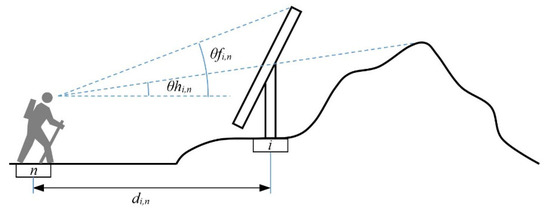 Figure 1. Lines of sight connecting the observer, in node n, to the PV facility and to the horizon.
The index can take values between 0 and 1, and represents the value per unit of the height Hpv above the skyline, as seen by an observer located at node n. When the whole facility (in terms of height) is below the skyline takes a value of 0, on the other hand, when the entire facility is above the skyline takes a value of 1. To evaluate it is necessary to determine the elevation angles and beforehand, as follows:
- First, we assume that observers can look in any direction, so it is necessary to determine the horizon line around each observation point or node n, whose geographical coordinates are known. That is, the horizon height must be evaluated for observer azimuth values from 0 to 360 sexagesimal degrees. The observer’s azimuth refers to the angle, measured on the horizontal plane, formed by the direction in which the observer is looking with respect to a reference direction. In our work, the azimuth value was 0 degrees when the observer was facing east and 90 degrees when facing north. After applying GIS tools, the result obtained, for each node n, is a raster dataset in which each cell i contains the value of the elevation angle of the line of sight connecting the observer’s eyes in node n to the global horizon beyond the area represented by the cell i. Consequently, all cells with the same azimuth value, will also take the same value of ;
- To obtain the elevation angle , visibility analysis GIS tools are applied at each node n. As result, a raster dataset is obtained in which each cell i contains the value of the elevation angle of the line of sight connecting the observer’s eyes in node n with the highest part of the possible PV facility placed in the cell i;
- Subsequently, by means of raster data layer processing techniques (map algebra) the index is determined using the expression (4).
For a single observer in node n, the value of APTi,n in cell i will take the value resulting from the product of the visibility height factor , the weighting factor wi,n as a function of distance di,n, the average observation time tn, and the term (1 + ). This last term has been introduced in order to give a higher degree of visibility to facilities that can be seen above the skyline. We have applied this methodology to routes that are mainly taken by walkers in periods of good weather with clear skies and high colour contrast (spring, summer and autumn seasons). Therefore, the visibility of the fraction of the PV plant that can be seen above the horizon line has received twice as much weight as the rest of the facility. The APTi,n calculation process is shown in Figure 2.
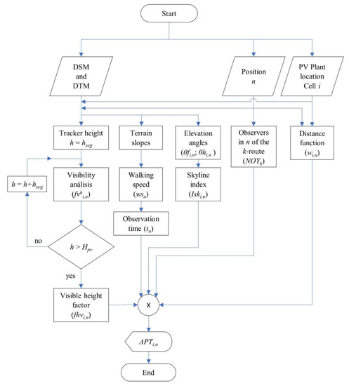
Figure 2.
APTi,n calculation flow-chart for PV plant placed in the area represented by cell i, and observers in the position represented by node n.
Taking into account the average annual number of observers that can circulate through node n of route k (NOYk), the cumulative value of APTi,n will be given by the expression (5).
2.2. Global Accumulated Perception Time
Finally, taking into account all the observation points or nodes n of route k and the number of observers NOYk travelling through each route, the cumulative value of APTi,k in cell i, will be given by the expression (6),
where Nn represents the total number of nodes or observation points on route k.
This process is repeated sequentially, analysing all possible routes (roads, path or trails used by the potential observers) in the area under study, so that for each cell i, the result of adding the APTi,k values of each route k is the global value of the accumulated perception time (GAPTi), as shown in (7),
where Nk represents the total number of routes in the study area.
The GAPTi values in each of the cells in the studied area are collected in a raster dataset, which can be visually analysed in the form of a map. In this way, it is possible to easily visualize those areas with a lower GAPT value which are therefore candidates for the installation of PV plants under an objective visibility criterion. Note that the purpose of the proposed methodology is to be able to choose the place within the study area where a new PV plant with certain characteristics can be built with the least observability by visitors who move along the routes in that area.
This methodology can be applied to tourist areas or areas with unique qualities where, due to their location or their relationship with the landscape, it is necessary to determine those sites where the presence of new PV plants would be less harmful in terms of the visual impact. A similar case is its application to areas close to historical sites and landmarks, since PV facilities visible from these locations can have a negative impact on the perception of their cultural value [39]. The visual impact in places with a great cultural heritage has become a controversial topic [40] and, in general, the methodology proposed in this work can be used for evaluating the construction of new PV plants in locations that, due to their cultural heritage and their cultural, historical or landscape value, have to be preserved [41].
3. Case Study
We have applied the proposed methodology to the region of La Rioja in northern Spain. Specifically, the selected area of study corresponds to the area crossed by the Way of St. James. Figure 3 shows, in the bottom right corner, the region of La Rioja, and the studied area. The Way of Saint James is a world-renowned pilgrimage route that runs through northern Spain, from the western range of the Pyrenees to the city of Santiago de Compostela, in the northwest of the country. In 1993 it was declared a World Heritage Site by UNESCO, forming part of the cultural legacy of Europe, one of the most varied in the world [42].
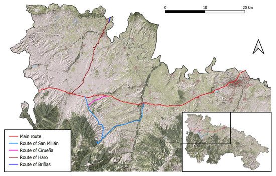
Figure 3.
Way of Saint James through La Rioja (Spain).
In the studied area, the Way of St. James does not have a single route, rather it has different variants or branches that run through different towns and places with great cultural richness close to the main route and where it is possible to visit sanctuaries, temples and other monuments that are part of the cultural heritage of the region. The main route crossing La Rioja was established at the beginning of the 11th century. In addition to the historical and cultural interest of the Way, the different routes in La Rioja cross through vineyards that constitute an environment of special landscape beauty. The five routes of the Way in La Rioja are shown in Figure 3 and these are: main route, route of San Millán, route of Cirueña, route of Haro, and route of Briñas.
In this work, the possible potential observers correspond to pilgrims walking along each of the five routes, while the inhabitants of the urban centres, included in the study area, have not been considered. Data related to pilgrimages have been taken from periodic statistical reports published by the Pilgrim’s Office in the city of Santiago de Compostela. For this work, data referring to pilgrimages during the year 2019 have been used [43]. In that year, about 190,000 pilgrims walked these routes of the Way.
A PV system with a two-axis tracker has been selected for the construction of new PV plants in this case study. Each system can support up to 10 kW of power, depending on the type of PV module installed. The height of such a tracker is not constant throughout the day and its value varies depending on the elevation angle of the sun (angle between the sun’s rays and the horizontal plane). The maximum height Hpv that can be reached by this facility is 6 m above the ground, mainly in the early and late hours of the day. This height was selected for this study because it is the most unfavourable value from the visibility criterion. The area occupied by a single tracker is approximately 625 m2, including the terrain corresponding to transit areas.
In the GIS tool the main input data are the DSM and the DTM of the area of study. According to data from the National Geographic Institute of Spain [44], the DSM was obtained from flights made during the summer of 2016. This geographic data is composed of a set of square cells with an initial size of 2.5 × 2.5 m. Using resampling techniques, the original DSM was converted to a DSM with a cell size of 25 × 25 m. We used the nearest neighbour interpolation as the resampling method, which is one of the fastest interpolation methods. With this method, each cell or pixel of the resampled raster data acquires the same value as its nearest neighbour in the original raster. Originally, the DTM had a cell size of 25 × 25 m; therefore, it was not necessary to apply sampling techniques. The final cell size was chosen according to the size occupied by a two-axis solar tracker with a capacity of 10 kW. In other words, each solar tracker would occupy the geographic area represented by a single cell in GIS.
4. Results and Discussion
In order to evaluate the values of the GAPT variable in the region under study, the stages described above in Section 2 have been followed:
- Using a GIS tool and considering the cell size of the DSM, equidistant nodes were generated every 25 m (dn = 25 m) along each route of the Way of St. James. The points corresponding to each of the five routes were collected in different vector data layers, in whose attribute tables, each node had associated data such as the average height above the ground of the observer’s eyes (1.61 m in this study), and the maximum height Hpv above the ground of the PV facility (Hpv = 6 m);
- GIS tools were used to obtain the value of the pilgrim’s walking speed wsn associated with each node n. This value was obtained applying expression (2). The value of walking speed was calculated for all the nodes of the five routes in the studied area;
- The average observation time, tn, was calculated for each node, dividing the real distance between consecutive nodes Dn by the value of the observer’s walking speed wsn at that node;
- With the suitable GIS tool, a Euclidean distance raster map was generated for each node n, what allows to generate a new raster dataset containing the weight factor wi,n;
- Several repeated visibility analyses were performed to calculate the visible height factor of the future PV plant placed in the cell i, following the methodology described in Section 2. Note that the length of the segment used in this case study was 1 m (hseg = 1 m) and, therefore, a set of six binary raster maps was obtained. Afterwards, using map algebra GIS tools, expression (3) was applied, obtaining a raster map with the values of the factor as a result, which represents the fraction of the PV facility located in the cell i, that can be seen from node n;
- The skyline index was evaluated using the expression (4). For each node n, two raster maps were obtained, each one storing the values of and , respectively, in cell i. Then, using map algebra techniques, the index was determined, which made it possible to give more weight to the visibility of future PV plants that could be seen above the skyline.
Next, taking into account the annual number of walkers traveling all the nodes of each of the five routes, NOYk, the expression (6) was applied, obtaining a raster map in which each cell i represented the value of the accumulated perception time APTi,k, achieved by the PV plant placed in that cell.
The volume of data in the raster format obtained in the calculation process was so high that R functions [45] were used to speed up this process and to automate access to the geo-algorithms integrated in QGIS from outside QGIS [46].
Finally, the expression (7) was applied to obtain the global value of accumulated perception time in each cell i (GAPTi). Applying the described methodology to the selected study area, the GAPT map shown in Figure 4 was obtained.
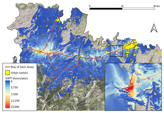
Figure 4.
GAPT map, in hours/year, of the study area.
In the area of study, the urban centres are represented by yellow polygons and the different routes of the Way of St James are represented by red lines. The cells that show the DEM as background (green and grey cells at the top and bottom of Figure 4) represent the areas that have a zero GAPT value and correspond to sites where the PV facilities are not visible from the routes, or to sites that are at a greater distance than the established limit of vision (10 km in our case study). These cells will be the best areas for the location of this type of solar facilities, from the point of view of their low observability from the routes of the Way of Saint James. The blue cells represent the lowest non-zero GAPT values, while the red cells represent the zones with the highest GAPT values and are therefore zones that should be avoided when it comes to the installation of PV plants. We can observe that the cells with higher GAPT values are relatively near the main route (route 1). The main reason is that it corresponds to the route most used by pilgrims traveling to Santiago de Compostela. The routes that generally cross geographic areas with gentle depressions and elevations do not have too many natural obstacles and PV plants in such areas can reach significant values of cumulative perception time.
The lower right corner of Figure 4 shows a zoom of the area marked by a black rectangle. It is an area with gentle mountains and low vegetation, therefore, there is a greater number of cells with high GAPT values. This is mainly due to the fact that a significant part of the facilities can be seen crossing the horizon line and having the sky as a background in these locations. Therefore, the observability of a PV plant such as the proposed one will be higher.
The results obtained provide accurate visibility maps with which it is easy to identify the locations where the installation of a future PV plant will have less visual impact for pilgrims walking along the Way of Saint James. The fundamental idea is to preserve the areas that surround and, above all, can be seen from the Way, so that they preserve its cultural legacy and previously held image.
In this case study, we have only analysed a 10 kW PV plant (each tracker occupies one cell of the map). Generally, the projected facilities will be much larger, and more cells will be required to cover the entire area occupied by the future facility. The solution to this problem is to select zones containing contiguous cells with low GAPT values.
5. Conclusions
The construction of new PV plants contributes to the reduction of CO2 emissions but does not have the support of all the parties involved. In areas that have a high landscape value or in tourist areas, this type of facility can be opposed by the population due to its visual impact. This work has presented a methodology, based on GIS, to determine the places where future PV facilities will have a greater or lesser visibility for a set of potential observers in movement, and its application to geographical areas with special landscape or cultural protection. The methodology is based on an objective measure: the accumulated perception time for all the potential observers.
The perception that observers have of this type of facility is estimated by means of a variable called Accumulated Perception Time, APTi,k. This variable represents the cumulative value of the possible hours per year in which the proposed PV plant, located in cell i, can be seen by observers travelling along all the observation points of route k. In order to make a more appropriate assessment of observability, two factors have been included in the calculation of APTi,k: the factor , which considers the visible part of the PV facility placed in the cell i, from observation point n, and the skyline index, , which takes into account the part of the facility that can be see above the horizon. This makes it possible to present a greater degree of visibility to facilities that can be seen partially or totally above the horizon.
By calculating the values obtained for the APTi,k variables of each route k in the area studied, the GAPTi variable is evaluated. This variable represents the global cumulative value of hours per year in which the future PV plant, placed in the cell i, can be seen by all observers travelling along all routes k in the area under study. It is possible to generate maps that graphically represent the value of the GAPT variable, by means of the use of GIS tools. With these maps, the agents involved in the construction of PV plants can easily identify those locations in the study area with lower GAPT values and which will therefore be more suitable for the installation of PV plants, based objectively on their observability.
As a case study, we have applied this methodology to one of the most famous pilgrimage routes. Specifically, the study area is the section of the Way of Saint James that crosses the region of La Rioja in northern Spain. The observers that have been considered correspond to the pilgrims that walk along all routes of the Way in this region. The result is a raster dataset that represents the value of the GAPT variable, in which it is possible to identify those places which have lower values and which, therefore, will be more suitable for the installation of PV plants based on their low observability from the Way of Saint James.
Some of the limitations of the proposed methodology, that will be addressed in future works, focus on the following issues:
- A high computational effort is required to achieve detailed results. Each visibility analysis for different heights of the PV facility produces a raster map.
- All the nodes of the routes have been considered as waypoints for the observers. In a more detailed analysis, a special treatment could be considered for some of these nodes corresponding to places on the Way of St. James where pilgrims usually stop on their way: viewpoints, fountains or rest areas. The APTi,n value for these nodes should be proportional to the average stopping time of pilgrims at such locations.
- The visual impact caused by glares from PV panels has not been taken into account.
The methodology described here is easily applicable to different routes, observers with different characteristics, and photovoltaic facilities with different dimensions, etc. In such cases, it would suffice to introduce the appropriate values of the factors that intervene in the calculation of the GAPT variable. The results obtained are easily interpretable and can be used by decision-makers (investors and local authorities) to plan new PV plants in areas with special cultural, historical or landscape value. The methodology can also be applied to other types of facilities (wind turbines, electricity pylons, communications antennas and buildings), taking appropriate values for the cell size and the maximum height of the projected facility.
Author Contributions
Conceptualization, L.A.F.-J. and E.Z.-A.; methodology, L.A.F.-J. and E.Z.-A.; software, E.Z.-A., P.J.Z.-S., M.M.-V., E.G.-G. and C.C.-V.; validation, P.J.Z.-S., M.M.-V., P.M.L.-S. and C.C.-V.; formal analysis, E.Z.-A., M.M.-V. and A.F.; investigation, P.J.Z.-S., P.M.L.-S., E.G.-G. and C.C.-V.; resources, P.M.L.-S., E.G.-G., A.F. and C.C.-V.; data curation, P.J.Z.-S., M.M.-V., P.M.L.-S., A.F. and C.C.-V.; writing—original draft preparation, E.Z.-A.; writing—review and editing, L.A.F.-J. and E.Z.-A.; visualization, L.A.F.-J., P.J.Z.-S., M.M.-V., P.M.L.-S., E.G.-G. and A.F.; supervision, L.A.F.-J.; project administration, L.A.F.-J.; funding acquisition, L.A.F.-J. All authors have read and agreed to the published version of the manuscript.
Funding
This research was funded by University of La Rioja and Banco Santander (REGI2020-28).
Institutional Review Board Statement
Not applicable.
Informed Consent Statement
Not applicable.
Data Availability Statement
Not applicable.
Conflicts of Interest
The authors declare no conflict of interest.
Abbreviations
| DEM | Digital Elevation Model |
| DSM | Digital Surface Model |
| DTM | Digital Terrain Model |
| GIS | Geographic Information System |
| PV | Photovoltaic |
| APTi,n | Accumulated perception time in cell i, with the observers located at node n (h/y) |
| APTi,k | Accumulated perception time in cell i by all observers moving along route k (h/y) |
| dn | Distance in the horizontal plane between nodes n and n + 1 (meters) |
| Dn | True distance between nodes n and n + 1 (meters) |
| di,n | Euclidean distance between cell i and node n (meters) |
| Visible height factor of a PV plant placed in cell i and viewed from node n | |
| Visibility factor of a PV plant of height h, placed in cell i and viewed from node n | |
| GAPTi | Global Accumulated Perception Time in cell i |
| h | Analysed height of the PV plant (meters) |
| Hpv | Maximum height of the PV plant (meters) |
| hseg | Segment length by which the height of the PV plant is increased in the visibility analysis |
| i | Geographic elemental area or cell with the possibility of housing a PV plant |
| Skyline index for a PV plant placed in cell i and viewed from node n | |
| k | Any route considered in the study area |
| n | Observation point or node contained in route k |
| Nk | Total number of routes in the study area |
| Nn | Total number of nodes on route k |
| NOYk | Annual number of potential observers moving along the route k |
| tn | Average observation time when the observer moves from node n to node n + 1 (hours) |
| Weighting factor calculated as a function of distance di,n | |
| Walking speed of the observer at node n (km/h) | |
| Angle of the terrain slope in the direction of travel of the observer | |
| Elevation angle of the line of sight between node n and the top of the PV plant in cell i | |
| Elevation angle of the line of sight connecting the observer’s eyes at n with the horizon, beyond cell i |
References
- Bachner, G.; Steininger, K.W.; Williges, K.; Tuerk, A. The economy-wide effects of large-scale renewable electricity expansion in Europe: The role of integration costs. Renew. Energy 2019, 134, 1369–1380. [Google Scholar] [CrossRef]
- Al Garni, H.Z.; Awasthi, A. Solar PV power plant site selection using a GIS-AHP based approach with application in Saudi Arabia. Appl. Energy 2017, 206, 1225–1240. [Google Scholar] [CrossRef]
- Carrión, J.A.; Estrella, A.E.; Dols, F.A.; Toro, M.Z.; Rodríguez, M.; Ridao, A.R. Environmental decision-support systems for evaluating the carrying capacity of land areas: Optimal site selection for grid-connected photovoltaic power plants. Renew. Sustain. Energy Rev. 2008, 12, 2358–2380. [Google Scholar] [CrossRef]
- Xu, Y.; Li, Y.; Zheng, L.; Cui, L.; Li, S.; Li, W.; Cai, Y. Site selection of wind farms using GIS and multi-criteria decision making method in Wafangdian, China. Energy 2020, 207, 118222. [Google Scholar] [CrossRef]
- Eroğlu, H. Multi-criteria decision analysis for wind power plant location selection based on fuzzy AHP and geographic information systems. Environ. Dev. Sustain. 2021, 23, 18278–18310. [Google Scholar] [CrossRef]
- Terkenli, T.; Skowronek, E.; Georgoula, V. Landscape and Tourism: European Expert Views on an Intricate Relationship. Land 2021, 10, 327. [Google Scholar] [CrossRef]
- Mouflis, G.D.; Gitas, I.Z.; Iliadou, S.; Mitri, G.H. Assessment of the visual impact of marble quarry expansion (1984–2000) on the landscape of Thasos island, NE Greece. Landsc. Urban Plan. 2008, 86, 92–102. [Google Scholar] [CrossRef]
- Ioannidis, R.; Koutsoyiannis, D. A review of land use, visibility and public perception of renewable energy in the context of landscape impact. Appl. Energy 2020, 276, 115367. [Google Scholar] [CrossRef]
- Cohen, J.J.; Reichl, J.; Schmidthaler, M. Re-focussing research efforts on the public acceptance of energy infrastructure: A critical review. Energy 2014, 76, 4–9. [Google Scholar] [CrossRef]
- Sibille, A.D.C.T.; Cloquell-Ballester, V.-A.; Cloquell-Ballester, V.-A.; Darton, R. Development and validation of a multicriteria indicator for the assessment of objective aesthetic impact of wind farms. Renew. Sustain. Energy Rev. 2009, 13, 40–66. [Google Scholar] [CrossRef]
- Bishop, I.D. The implications for visual simulation and analysis of temporal variation in the visibility of wind turbines. Landsc. Urban Plan. 2019, 184, 59–68. [Google Scholar] [CrossRef]
- Maslov, N.; Claramunt, C.; Wang, T.; Tang, T. Method to estimate the visual impact of an offshore wind farm. Appl. Energy 2017, 204, 1422–1430. [Google Scholar] [CrossRef]
- Torres-Sibille, A.d.C.; Cloquell-Ballester, V.A.; Cloquell-Ballester, V.A.; Artacho Ramírez, M.Á. Aesthetic impact assessment of solar power plants: An objective and a subjective approach. Renew. Sustain. Energy Rev. 2009, 13, 986–999. [Google Scholar] [CrossRef]
- Chiabrando, R.; Fabrizio, E.; Garnero, G. The territorial and landscape impacts of photovoltaic systems: Definition of impacts and assessment of the glare risk. Renew. Sustain. Energy Rev. 2009, 13, 2441–2451. [Google Scholar] [CrossRef]
- Moser, D.; Vettorato, D.; Vaccaro, R.; Del Buono, M.; Sparber, W. The PV Potential of South Tyrol: An Intelligent Use of Space. Energy Procedia 2014, 57, 1392–1400. [Google Scholar] [CrossRef] [Green Version]
- Munkhbat, U.; Choi, Y. GIS-Based Site Suitability Analysis for Solar Power Systems in Mongolia. Appl. Sci. 2021, 11, 3748. [Google Scholar] [CrossRef]
- Rodrigues, M.; Montañés, C.; Fueyo, N. A method for the assessment of the visual impact caused by the large-scale deployment of renewable-energy facilities. Environ. Impact Assess. Rev. 2010, 30, 240–246. [Google Scholar] [CrossRef]
- Manchado, C.; Gomez-Jauregui, V.; Lizcano, P.E.; Iglesias, A.; Galvez, A.; Otero, C. Wind farm repowering guided by visual impact criteria. Renew. Energy 2019, 135, 197–207. [Google Scholar] [CrossRef]
- Hurtado, J.; Fernández, J.; Parrondo, J.L.; Blanco, E. Spanish method of visual impact evaluation in wind farms. Renew. Sustain. Energy Rev. 2004, 8, 483–491. [Google Scholar] [CrossRef]
- Molina-Ruiz, J.; Sánchez, M.J.M.; Pérez-Sirvent, C.; Serrano, M.L.T.; Lorenzo, M.L.G. Developing and applying a GIS-assisted approach to evaluate visual impact in wind farms. Renew. Energy 2011, 36, 1125–1132. [Google Scholar] [CrossRef]
- Wróżyński, R.; Sojka, M.; Pyszny, K. The application of GIS and 3D graphic software to visual impact assessment of wind turbines. Renew. Energy 2016, 96, 625–635. [Google Scholar] [CrossRef]
- Garcia-Garrido, E.; Lara-Santillan, P.; Zorzano-Alba, E.; Mendoza-Villena, M.; Zorzano-Santamaria, P.; Fernandez-Jimenez, L.A.; Falces, A. Visual impact assessment for small and medium size PV plants. In Proceedings of the 12th WSEAS International Conference on Electric Power Systems, High Voltages, Electric Machines, Prague, Czech Republic, 24–26 September 2012; pp. 57–61. [Google Scholar]
- Fernandez-Jimenez, L.A.; Mendoza-Villena, M.; Zorzano-Santamaria, P.; Garcia-Garrido, E.; Lara-Santillan, P.; Zorzano-Alba, E.; Falces, A. Site selection for new PV power plants based on their observability. Renew. Energy 2015, 78, 7–15. [Google Scholar] [CrossRef]
- Florio, P.; Probst, M.C.M.; Schüler, A.; Roecker, C.; Scartezzini, J.-L. Assessing visibility in multi-scale urban planning: A contribution to a method enhancing social acceptability of solar energy in cities. Sol. Energy 2018, 173, 97–109. [Google Scholar] [CrossRef]
- Pham, V.-M.; Van Nghiem, S.; Van Pham, C.; Luu, M.P.T.; Bui, Q.-T. Urbanization impact on landscape patterns in cultural heritage preservation sites: A case study of the complex of Huế Monuments, Vietnam. Landsc. Ecol. 2021, 36, 1–26. [Google Scholar] [CrossRef]
- Ashrafi, B.; Kloos, M.; Neugebauer, C. Heritage Impact Assessment, beyond an Assessment Tool: A comparative analysis of urban development impact on visual integrity in four UNESCO World Heritage Properties. J. Cult. Herit. 2021, 47, 199–207. [Google Scholar] [CrossRef]
- QGIS. A Free and Open Source Geographic Information System. Available online: https://www.qgis.org/en/site/ (accessed on 28 January 2021).
- Fisher, P.F. Extending the applicability of viewsheds in landscape planning. Photogramm. Eng. Remote Sens. 1996, 62, 1297–1302. [Google Scholar]
- UNESCO. Routes of Santiago de Compostela: Camino Francés and Routes of Northern Spain. Available online: https://whc.unesco.org/en/list/669 (accessed on 10 September 2021).
- Polidori, L.; El Hage, M. Digital Elevation Model Quality Assessment Methods: A Critical Review. Remote. Sens. 2020, 12, 3522. [Google Scholar] [CrossRef]
- Bishop, I. Testing perceived landscape colour difference using the Internet. Landsc. Urban Plan. 1997, 37, 187–196. [Google Scholar] [CrossRef]
- Ogburn, D.E. Assessing the level of visibility of cultural objects in past landscapes. J. Archaeol. Sci. 2006, 33, 405–413. [Google Scholar] [CrossRef]
- Fisher, P.F. Probable and fuzzy models of the viewshed operation. In Innovations in GIS; CRC Press: Boca Raton, FL, USA, 1994; pp. 161–175. [Google Scholar]
- Weigel, J. Kompensationsflächenberechnung für Freileitungen. Available online: https://www.yumpu.com/de/document/read/6771445/kompensationsflachenberechnung-fur-freileitungen (accessed on 31 August 2021).
- Paul, H.-U.; Uther, D.; Neuhoff, M.; Winkler-Hartenstein, K.; Schmidtkunz, H.; Grossnick, J. GIS-gestütztes Verfahren zur Bewertung visueller Eingriffe durch Hochspannungsfreileitungen. Nat. Und Landschaftsplan. Z. Für Angew. Okol. 2004, 36, 139–144. [Google Scholar]
- Pérez, J.M.; Vallejo, I.; Álvarez-Francoso, J.I. Estimated travel time for walking trails in natural areas. Geogr. Tidsskr.-Danish J. Geogr. 2017, 117, 53–62. [Google Scholar] [CrossRef]
- Fontani, F. Application of the Fisher’s “Horizon Viewshed” to a proposed power transmission line in Nozzano (Italy). Trans. GIS 2016, 21, 835–843. [Google Scholar] [CrossRef]
- Caha, J.; Rášová, A. Line-of-Sight Derived Indices: Viewing Angle Difference to a Local Horizon and the Difference of Viewing Angle and the Slope of Line of Sight. Lect. Notes Geoinf. Cartogr. 2015, 211, 61–72. [Google Scholar] [CrossRef]
- Serra, J.; Llinares, C.; Iñarra, S.; Torres, A.; Llopis, J. Improvement of the integration of visually impacting architectures in historical urban scene, an application of semantic differencial method. Environ. Impact Assess. Rev. 2019, 81, 106353. [Google Scholar] [CrossRef]
- Jerpåsen, G.B.; Larsen, K.C. Visual impact of wind farms on cultural heritage: A Norwegian case study. Environ. Impact Assess. Rev. 2011, 31, 206–215. [Google Scholar] [CrossRef]
- CETS 199—Council of Europe Framework Convention on the Value of Cultural Heritage for Society. Available online: https://rm.coe.int/1680083746 (accessed on 6 September 2021).
- European Commission Directorate-General for Research and Innovation. Preserving our Heritage, Improving our Environment. Volume I, 20 Years of EU Research into Cultural Heritage; Chapuis, M., Ed.; Publications Office of the European Union: Luxembourg, 2009; Available online: https://data.europa.eu/doi/10.2777/17146 (accessed on 3 September 2021).
- Informe Estadístico. 2019. Available online: http://oficinadelperegrino.com/wp-content/uploads/2016/02/peregrinaciones2019.pdf (accessed on 24 August 2021).
- Instituto Geográfico Nacional. Available online: https://www.ign.es/web/ign/portal (accessed on 4 September 2021).
- R Development Core Team. The R project for statistical computing, R version 3.5.2. 2018. Available online: https://www.r-project.org (accessed on 2 September 2021).
- Lovelace, R.; Nowosad, J.; Muenchow, J. Geocomputation with R; Chapman and Hall/CRC: Boca Raton, FL, USA, 2019. [Google Scholar]
Publisher’s Note: MDPI stays neutral with regard to jurisdictional claims in published maps and institutional affiliations. |
© 2022 by the authors. Licensee MDPI, Basel, Switzerland. This article is an open access article distributed under the terms and conditions of the Creative Commons Attribution (CC BY) license (https://creativecommons.org/licenses/by/4.0/).