Article

Synchronized Assessment of Bridge Structural Damage and Moving Force via Truncated Load Shape Function

1
School of Traffic and Logistics Engineering, Wuhan University of Technology, Wuhan 430034, China
2
School of Transportation and Civil Engineering, Nantong University, Nantong 226019, China
3
MOE Key Lab of Disaster Forecast and Control in Engineering, Jinan University, Guangzhou 510632, China
4
State Key Laboratory for Health and Safety of Bridge Structures, Wuhan 430034, China
5
China Railway Bridge Science Research Institute, Ltd., Wuhan 430034, China
*
Author to whom correspondence should be addressed.
Appl. Sci. 2022, 12(2), 691; https://doi.org/10.3390/app12020691
Submission received: 18 November 2021 / Revised: 22 December 2021 / Accepted: 5 January 2022 / Published: 11 January 2022
(This article belongs to the Special Issue Advanced and Innovative Technologies for Structural Health Monitoring)

Abstract

:
Moving load and structural damage assessment has always been a crucial topic in bridge health monitoring, as it helps analyze the daily operating status of bridges and provides fundamental information for bridge safety evaluation. However, most studies and research consider these issues as two separate problems. In practice, unknown moving loads and damage usually coexist and influence the bridge vibration synergically. This paper proposes an innovative synchronized assessment method that determines structural damages and moving forces simultaneously. The method firstly improves the virtual distortion method, which shifts the structural damage into external virtual forces and hence transforms the damage assessment as well as the moving force identification to a multi-force reconstruction problem. Secondly, a truncated load shape function (TLSF) technique is developed to solve the forces in the time domain. As the technique smoothens the pulse function via a limited number of TLSF, the singularity and dimension of the system matrix in the force reconstruction is largely reduced. A continuous beam and a three-dimensional truss bridge are simulated as examples. Case studies show that the method can effectively identify various speeds and numbers of moving loads, as well as different levels of structural damages. The calculation efficiency and robustness to white noise are also impressive.

1. Introduction

Accurate statistics regarding moving loads and structural damage are two very significant factors for bridge health monitoring. Identified loads can provide a vital basis for traffic studies and traffic control, while the damage assessment can guide ongoing bridge maintenance and design code calibration. Many studies have been investigated to address both of these assessment problems. However, most of the previous studies consider the two problems separately: either the structural damage is determined with the load characteristic to be known, or the moving load is identified on a bridge with complete structural condition (damage information). In most practical cases, unknown structural damages and unknown moving loads coexist and simultaneously influence the responses of the bridge structure. The synchronized identification of moving load and structural damage hence becomes an interesting topic.
In the theoretical research, scholars have carried out extensive studies on the detection of structural damages and the identification of moving forces. Direct detection techniques are widely studied and used, such as the weight-in-motion [1] or bridge weight-in-motion system [2] to monitor moving loads, unmanned aerial vehicles [3], terrestrial laser scanning [4], and ultrasonic waves [5] etc. to detect surface and internal damages of bridges. The advantages of these types of technique are that they can intuitively reflect target information with incomplete structure information and have a good efficiency in evaluating localized damaged areas. On the other hand, the drawbacks are also obvious. As the detection is noncontinuous, it is unable to detect structural changes during the inspection interval. In addition, it is difficult to monitor overall structure statues. In comparison, indirect techniques take the vehicle–bridge interaction as an “excitations-structure-responses” vibrational system, where variation of excitations and structure characteristics leads to different dynamic responses [6]. In this way, structural damage and moving force can be identified via solving the first and second kind of structural dynamic inverse problem, respectively. Compared to direct detection techniques, these techniques provide continuous monitoring by attaching various types of vibrational sensors and are flexible in detecting the local and overall conditions of the structure.
For moving force identification (MFI), existing methods could be mainly categorized into four categories, namely, direct methods, regularization methods, basis function methods, and intelligence algorithms. The direct methods are essentially solving linear equations, which inevitably face the ill-conditioned problem. Regularization methods and basis function expansions are mostly used to improve this problem. The regularization method is used to introduce reasonable additional information as the constraint of the original problem, which is also known as the penalty function, to improve the ill-posed nature of the original problem such as L2 norm regularization [7] and sparse regularization [8]. The basis function expansions use a specific function system to expand the unknown load and then transform the MFI problem into the selection problem of the basis function coefficient, while the number of the basis function is regarded as the regularization parameter. Various types of basis functions have been proposed, including trigonometric functions [9], spline functions [10], wavelet functions [11] shape functions [12], etc. In the studies of intelligence algorithms, MFI is usually regarded as a mathematical optimization problem or a learning-application process. The former solves the problem by constructing appropriate objective functions and choosing efficient optimization algorithms, such as the Firefly algorithm [13] and particle swarm optimization [14]. The latter establishes the relationship between the moving force and response via neural network training; hence the force could be inversely determined via response once the network reaches a certain accuracy.
In terms of structural damage identification (SDI), dynamic fingerprint-based methods and dynamic signal-based methods have been studied. Since the dynamic fingerprints, such as frequencies, mode shapes, frequency response functions, will change when the structure is damaged, it is able to detect damages via monitoring the variation of the fingerprints. However, these parameters are not sensitive to minor damages. In order to effectively highlight the changes caused by minor damage, more types of fingerprints have been proposed on the basis of mode shapes, such as the modal confidence factor, curvature mode, modal strain energy etc. [15,16,17,18]. However, errors in modal parameter measurement and noise pollution may inevitably make the change in these features difficult to evaluate. On the other hand, signal-based methods detect damages via distinguishing different dynamic responses. As the structural response is the result of the combined action of excitation and structural attribute, the variation of response only comes from the structural parameter change under similar excitation. The response signal can be processed in the time domain, frequency domain and frequency–time domain. The corresponding techniques include time series analysis techniques [19], power spectral density estimation [20], wavelet transformation [21] etc. It is worth noting that for signal-based methods, the environmental influence should not be overlooked; temperature changes, especially in long-term monitoring, seriously affect the accuracy of identification. Huang et al. [22] proposed an autoregressive (AR) time series model with a two-step artificial neural network (ANN) to determine damage under temperature variations, which extracted the first three-order coefficients of the AR model as damage feature and utilized ANN models to compensate the detrimental temperature changes.
It is apparent that most of the reviewed MFI methods require determined structure information to establish the correspondence between moving force and structural response, while the signal-based SDI methods need a similar excitation in order to guarantee the response variation solely caused by structural damage. These methods could be difficult to practice on bridges where unknown moving forces and structural damage coexist. The synchronized detection of both moving forces and structural damages has become vital. Zhu and Law [23] presented a method for damage detection of a simply supported bridge, in which the vehicles–bridge interaction forces and the structural damages were identified from the measured responses in a sequence of iteration without prior moving loads knowledge. Zhang and Law [24] assessed the condition of structures under unknown support excitation, which modeled the excitation as orthogonal polynomial approximations. A simultaneous identification method of moving masses and damages was presented via the virtual distortion method (VDM) [25], in which the damage was modified to virtual distortions and identified with moving load. Compared to other methods, the biggest advantage of VDM is that it unifies the solving path of SDI and MFI, which immensely simplifies the complexity of the method and greatly improves the computational efficiency [26].
Taking this advantage into account, an efficacious synchronized assessment method of moving force and structural damages is presented in this paper. Based on VDM, the synchronized identification of damage and moving forces are transformed to multiple forces identification and is solved using the Duhamel Integral. In order to reduce the singularity, a truncated load-shape function (TLSF) is developed to enhance the Duhamel Integral. Two numerical examples are presented to validate the proposed method. Various cases that consider the influence of force, velocity, number, damage severity, location, sensor position, and noise measurement to the identification accuracy and efficiency have been studied.

2. Synchronized Assessment Method

2.1. Forward Problem

VDM is a quick reanalysis method [27]. When the response of the original structure is given, the VDM allows the response of the modified structure to be quickly calculated without a time-consuming full structural simulation. Instead, this is conducted by adding the response caused by this modification-related virtual distortion. Theoretically, the modification in a finite element is represented by the equivalent pseudo-loads that are applied in its DOFs. In this way, a stiffness-related modification, such as structural damage, can be performed in the form of equivalent virtual forces or virtual distortions of the affected element. As a result, instead of considering a modified structure subjected to external excitation, the VDM considers the original structure subjected to certain virtual forces and the same external excitation, respectively, and both of these systems share the same dynamic responses.
Assuming the damage as linear stiffness decreasing, we can define ζ i as the damage ratio of the i t h element:
ζ i = k i d / k i o
where k i o   and   k i d represent the stiffness matrixes of the i t h element before and after damage. Hence, using the nodal displacement vector of the i t h element v i , it can express the nodal force vectors before and after damage p i o   and   p i d , respectively:
p i d = k i d v i = ζ i k i o v i = ζ i p i o
Therefore, the nodal force variation of the damaged and intact elements, namely the virtual force vector p i e yields:
p i e = p i o p i d = ( 1 ζ i ) k i o v i = ( 1 ζ i ) p i o
Assuming ϕ i j as the j t h basic distortion vector of the i t h element, there is p i o = j k i o ϕ i j = j λ i j o according to the Eigen equation of k i o , where λ i j o is the basic nodal force vector of the intact element. Equation (3) is also performed to:
p i e = j ( 1 ζ i ) k i o ϕ i j = j λ i j e
where λ i j e is the basic virtual force vector of the damaged element. This equation reveals the physical meaning of virtual force, which is determined by the basic distortion of the element. For example, a two-dimensional beam element has three situations of distortion: axial compression or tension, pure bending and bending, plus shearing. Accordingly, its virtual force contains axial force, shear force, and bending moment.
Expanding Equation (4) to global coordinate, if the coordinate transformation matrix of the i t h   element is named as T i , the i t h virtual force vector p i e can be performed in the global coordinate as the product of p i e and the transpose of T i . Hence the global virtual force vector containing multiple damages is obtained:
P e = i T i T p i e = i j T i T λ i j e
Similarly, the global nodal force vectors of the damaged structure P d and intact structures P o are i T i T p i d   and   i T i T p i o , respectively. It is not difficult to find the relationship between P d ,   P o   and   P e :
P d = P o P e
Therefore, the motion equation of a damaged bridge subjected to a moving force is
M V ¨ + C V ˙ + K d V = F
where M ,   C ,   and   K d are the global mass, damping, and stiffness matrices, F is the excitation force vector, V , V ˙ ,   and   V ¨ are the global displacement, velocity, and acceleration vectors, respectively. It is worth noting that the term K d V actually presents the global nodal forces P d . After being substituted by Equation (6) and transposition, Equation (7) is transformed to:
M V ¨ + C V ˙ + P o = F + P e
where P o donates the global nodal forces K V of the intact structure, as stated before. Therefore, Equation (7) can be turned into the motion equation of the intact bridge subjected to the same moving force as well as the global virtual force:
M V ¨ + C V ˙ + K V = F + P e
In this way, the assessment of structural damage and unknown moving force is transformed to the identification problem of the unknown moving force and the virtual force of the damaged element. This transformation has improved the identification mechanism, unifying the first and second inverse problems to the second inverse problem.

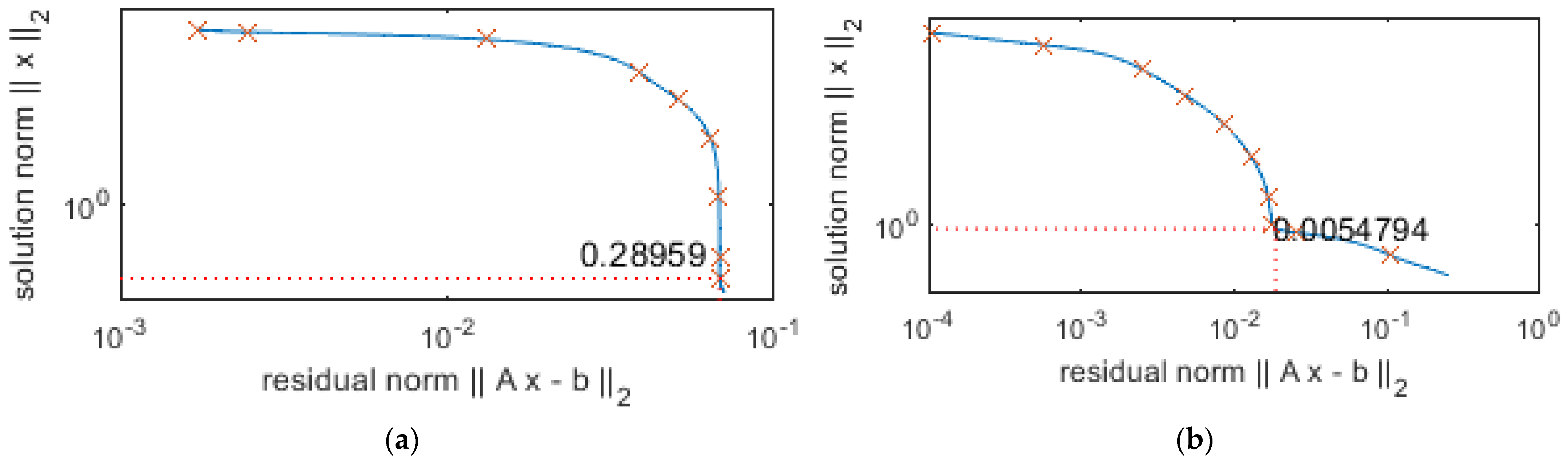
2.2. Inverse Problem

Considering the bridge as a linear system, the dynamic response of the bridge can be generated from the Duhamel Integral if the initial condition is zero [28]. Using the discrete form of the Duhamel Integral, the response vector Y caused by the moving force and global virtual force is:
Y = I F F + I e P e = I [ F P e ]
The first term refers to the response of the intact bridge subjected to the moving force, I F is the impulse response matrix of F . The second term is the response of the intact bridge subjected to the global virtual force, I e is the impulse response matrix caused by P e . Substituting Equation (5), Equation (10) is elaborated as:
[ Y 1 Y n ] = [ I F 1 I 11 1 I i j 1 I F 2 I 11 2 I i j 2 I F n I i j n ] [ F λ 11 e λ i j e ]
where Y = [ Y 1 Y n ] T is the response vector of the damaged structure, including n measured Y n . I is a partitioned matrix constituted by Toeplitz matrices I F n and I i j n , which represent the impulse response of the n t h measure point of the intact structure subjected to the impulse force of F and λ i j e , respectively. To guarantee the unique solution of this equation, n i × j + 1 . Therefore, the unknowns can be calculated from the inversion of Equation (11).
[ F λ 11 e λ i j e ] = I 1 Y
However, in practical cases I is very sensitive to noise, the metering noise is likely to cause an ill-conditioned problem in Equation (12). In addition, the dimension of I is huge when dealing high sampling rate or long-term measurement, which makes it difficult to be calculated.
Introducing a truncated load shape function (TLSF) can significantly restrain the influences caused by the problems above. TLSF compares the time history of excitation force to the span of a ‘finite element beam’. Consulting the concept of the shape function in the finite element method, the amplitude of the moving force F is regarded as the displacement of the beam, which can be calculated via the load shape function.
F = N γ F
where N is the load shape function matrix and γ F is the fitting coefficient vector. Similarly, λ i j e could also be expressed as:
λ i j e = N γ i j
Substituting Equations (13) and (14) to Equation (12), the identification of an unknown moving force and virtual forces is turned into the identification of a fitting coefficient:
Y = I [ N N N N ] [ F λ 11 e λ i j e ] = [ R F 1 R 11 1 R i j 1 R F 2 R 11 2 R i j 2 R F n R i j n ] [ γ F γ 11 γ i j ] = R Γ
The product of the impulse response matrix I as well as the load shape function matrix N could be collectively called influence matrix R . Its physical meaning is defined as the impulse response of intact structure caused by the shape function. Γ = [ γ F γ i j ] T is the coefficient vector. In practice, this response attenuates rapidly due to the influence of structural damping, and its effective value only takes a small proportion in the whole sampling time. Therefore, defining a truncated value μ :
μ = s t s t + δ R i j n ( : , h ) 1 T R i j n ( : , h )
which represents the ratio of the sum of the effective elements of each column of R i j n to the sum of all elements of the column. R i j n ( : , h ) represents the element in the hth column of R i j n , st is the first non-zero element in the column, and δ is defined as the effective length. Generally, μ is set as 90%~95% according to the decay rate of the impulse response. Then the matrices R are simplified and reconstituted into a diagonal matrix, which is called the TLSF matrix Λ . Substituting the TLSF matrix to Equation (15), the fitting coefficients can be easily obtained:
Γ = Λ 1 Y
Comparing the impulse response matrix I , influence matrix R , and TLSF   matrix   Λ , their dimensions are ( s n × s n ) ,   ( s α × 2 m n ) ,   a n d   ( s n × 2 m n ) ,   respectively , where s is the sampling number, n is the number of sensors, and m is the number of TLSFs. By using TLSF, the number of columns in I is reduced from s α to 2 m α . Besides, TLSF can extract the effective values of R and decrease the load steps during calculating Λ , hence further lowering the computing cost. Furthermore, because smooth TLSF is used to fit the pulse response, the singularity values in Λ are more balanced than those in I , which makes Equation (17) have higher robustness in the face of noise and need no further regularization.

2.3. Reconstruction of Moving Force and Structural Damage

Once the TLSF coefficient vector Γ is obtained, the moving force and basic virtual forces are able to be reconstructed via Equations (13) and (14).
Furthermore, the damage ratio could be calculated by the ratio of λ i j 0 λ i j e and λ i j o :
ζ i = λ i j 0 λ i j e λ i j o
Herein, the basic nodal force of the intact element λ i j o can also be calculated from the flexible use of the Duhamel Integral:
λ i j o = I i j i b f F
where I i j i b f represents the impulse response matrix of the j t h basic nodal force of the i t h intact element respected to the moving force F .

3. Numerical Validations

Two numerical examples are presented in this paper. The first example is a two-span continuous beam subjected to a fixed force, which is proposed to validate the efficiency and robustness of TLSF. The second example is a 3D truss bridge with damage in the hanger, subjected to 2-axle moving forces, which is used to validate the stability of the proposed synchronized assessment method.

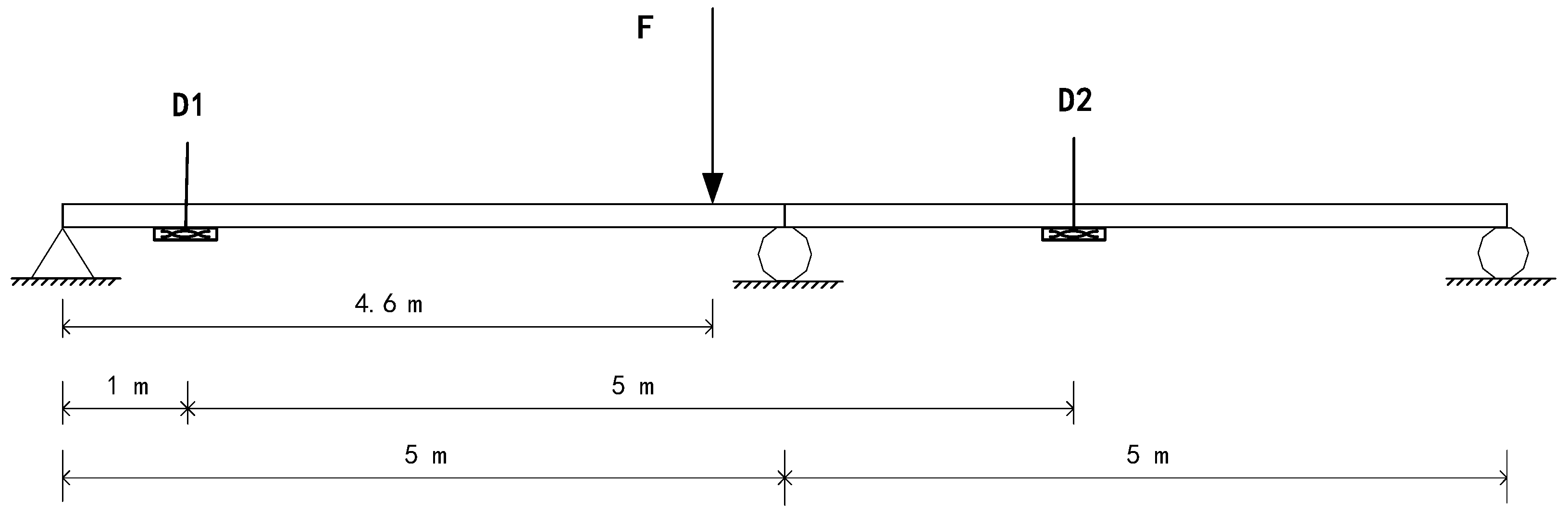
3.1. Continuous Beam Example

A two-span continuous beam is established, as shown in Figure 1. The span length is 5 m. The cross-section is an I-section with an area of 1.2 × 10 3   mm 2 and an inertia moment of 1.94 × 10 6   mm 4 . The Elastic modulus is 210 GPa, and the density is 7800   kg / m 3 . A fixed periodic load is applied at 4.6 m from the left end. The displacement responses are obtained from D1 and D2, respectively. The Rayleigh damping coefficients are set as 0.0822 and 0.0046.
A harmonic force and a square wave force is applied, respectively, and the responses of D1 and D2 are polluted by 5% white noises [8]:
Y n o i s e = Y + l e v e l × 1 χ i = 1 χ | Y | × r a n d o m
where Y n o i s e is the responses with noise, l e v e l is the noise level, χ   is   the   element   number   of   Y .   r a n d o m is a standard normal distribution vector. The time history of the force and responses are shown in Figure 2. The total measuring time is 5 s, and the sampling rate is 200 Hz.
As described before, the excitation force should be fitted by the TLSF according to Equation (13). Defining the frequency of LSF f L S F as:
f L S F = f s / 2 l
where f s is the sampling rate. l is the length of each TLSF. During the total measuring time T, there will be m TLSFs:
T × f s = l × m
f L S F is required to not be smaller than the main range of frequency of the unknown force in order to simulate all its details. In forced vibration, the frequency of unknown excitation closes to the frequency of the structural responses. Using the fast Fourier transformation of the response, the main frequency of the structural response is determined below 5 Hz. Hence f L S F is defined as 5 Hz in this case, l and m are calculated as 20 and 50, respectively. Therefore, the dimension of the influence matrix R is 1000 × 100 , which is 10 times smaller than the dimension of impulse response matrix I ( 1000 × 1000 ) . It is worth noting that the physical meaning of influence matrix R is the structural response due to LSF, which is usually obtained by finite element simulation. In this case, the time step that should be calculated is 1000. By introducing TLSF, defining the truncated value μ as 90% according to the damping effect, the effective length δ is calculated as 64. In this way, the calculation time step can be reduced to 64, and the affective dimension of TLSF matrix Λ can be decreased to 64 × 100 . In addition, because the TLSF smooth the impulse response, the singularity of Λ is small. Figure 3 show the L-curve of Λ   a n d   I with respect to the displacement response with noise. It is obvious that with the improvement of TLSF, no typical corner is found in the L-curve, even with 5% white noise in the measurement. This proves that TLSF can significantly enhance the condition of the matrix without a regularization procedure.
The determined results are presented in Figure 4. The relative percentage error (RPE) is defined in Equation (23), the results are listed in Table 1.
RPE = i | F i d e n t i f i e d F t r u e | F t r u e × 100 %
Generally, all the cases have been identified. No ill-conditioned problem is found even without regularization. The following is the discussion on different influencing factors.
(1)
The relative position of the response
The results of both types of forces illustrate that the recognition via D1 presents better accuracy than that via D2. Observing the relative position of D1 and D2, it can be found that D1 is on the same span with force, while D2 is on the other span. The error is caused by the restraining effect of the mid-span support to small forces. Due to the TLSF response matrix, Λ is constituted of the responses excited by the small TLSFs, the inhibition of mid-span support is amplified. This results in a distortion in Λ , and hence leads to a large error in determination during the inversion of Equation (17).
(2)
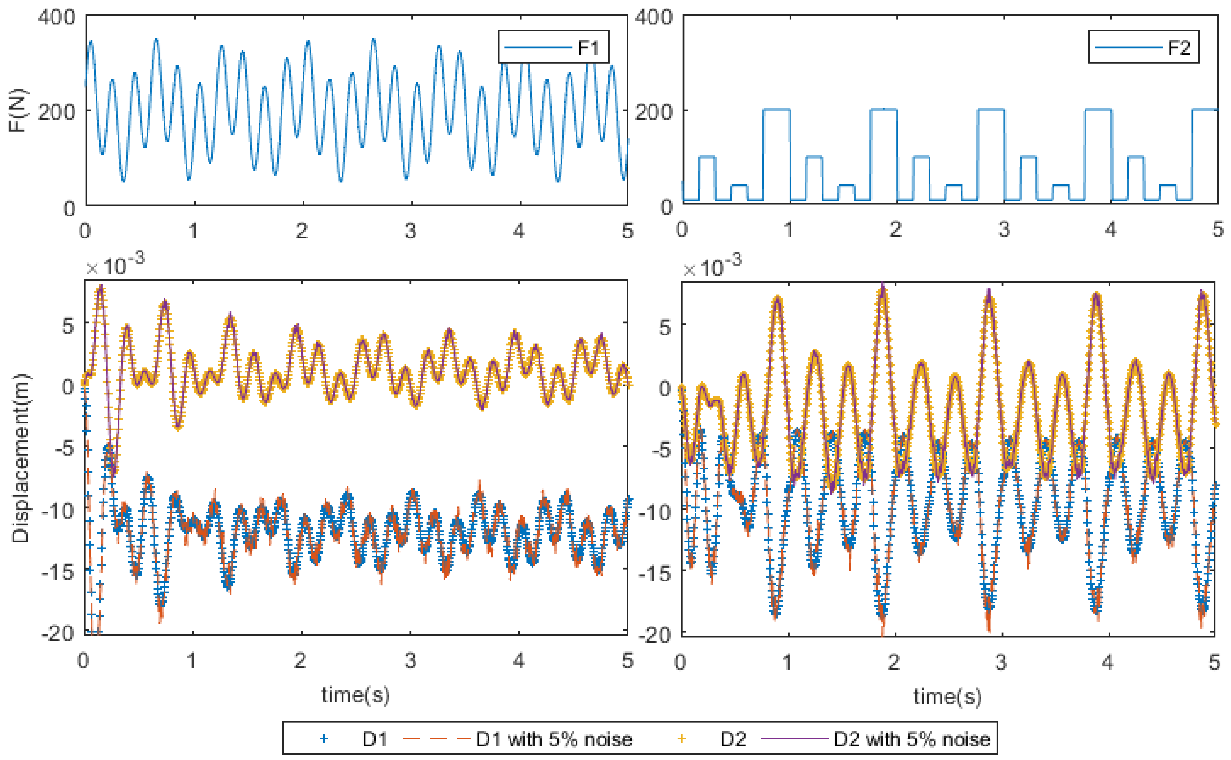
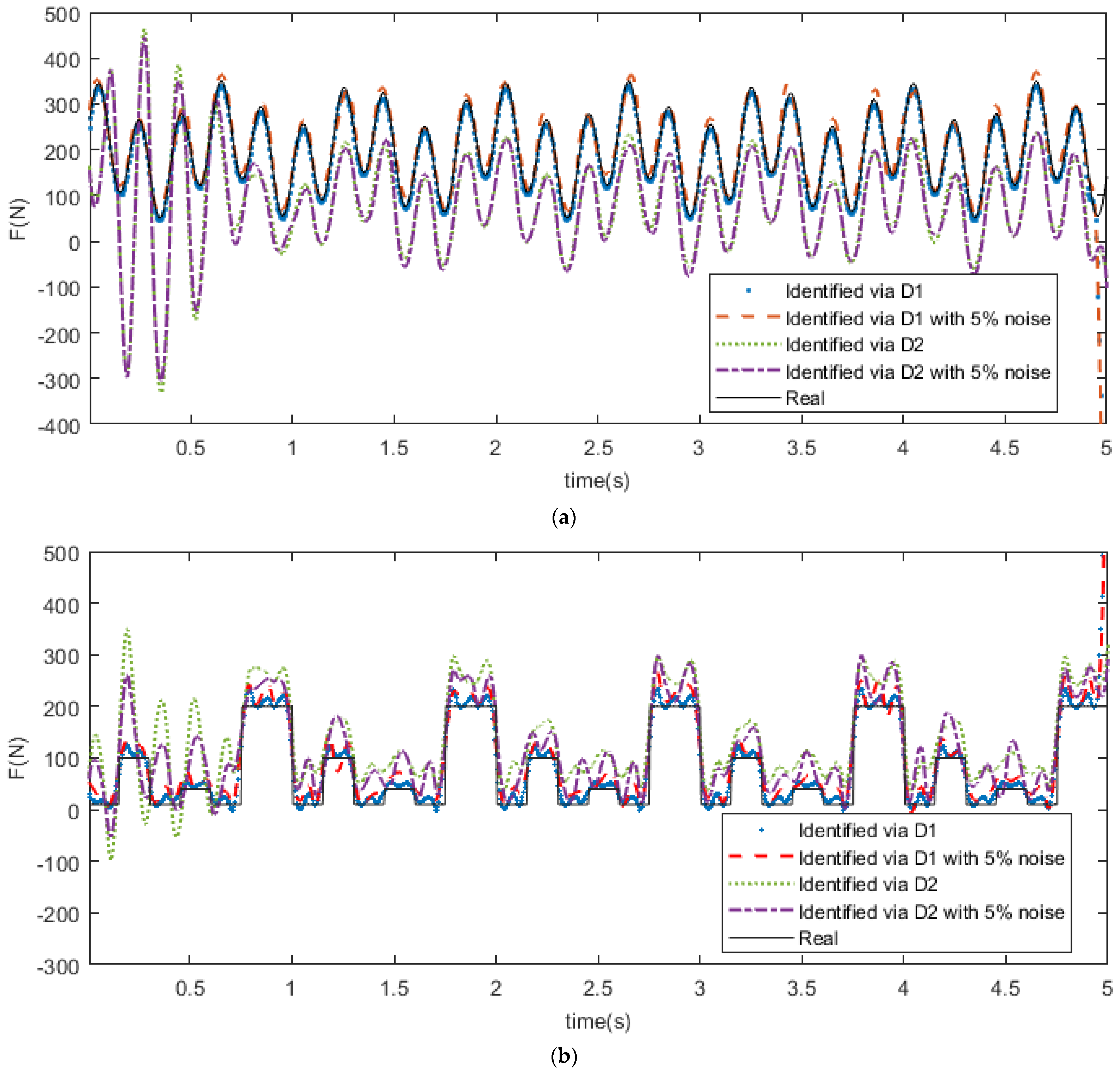
The type of the excitation force
Comparing Figure 4a,b, it is found that both the harmonic and square wave forces can be determined, and the accuracy of harmonic force is better. Taking the results through D1 as an example, the curve of the identified harmonic force closely follows the true force, while the curve of identified square wave force has visible fluctuations around the true force, especially at the corner when the force rapidly changes. This is because the large difference and discontinuity of the square wave force misled the method to determine the force as an ‘impulse force’ and hence produce a mutation at the corner.
(3)
The measurement noises
The cases containing noises have shown that measurement noises only affect the accuracy of the peak recognition in a small amplitude, and the impact on the overall curvature is negligible. The robustness of the proposed method to noise is further proved.

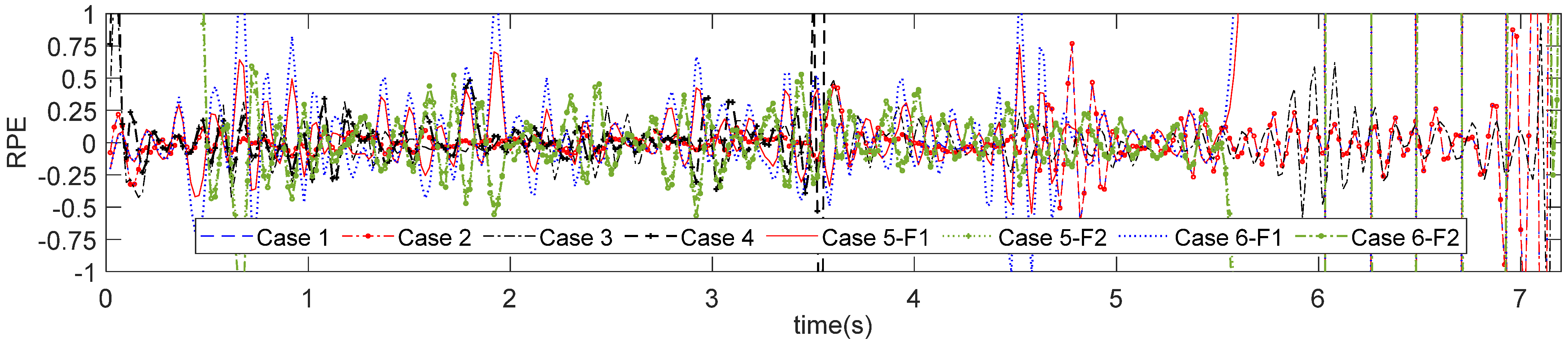
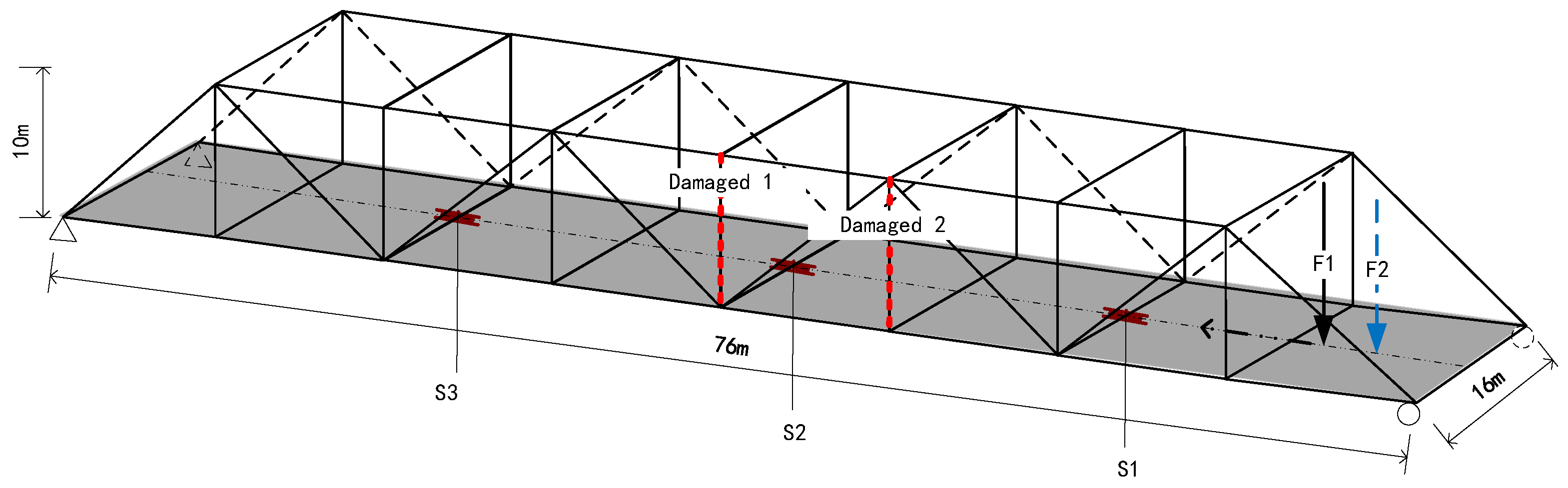
3.2. Truss Bridge Example

A three-dimensional truss bridge is established, as shown in Figure 5. The following parameters are designed: the main girders are a 32 b steel I-beam, the truss members are 50 mm diameter steel rods, the bridge deck is a 400 mm thick concrete slab. The Young’s modulus of steel and concrete are 210 GPa and 35 GPa; the densities are 7850   kg / m 3   and   2500   kg / m 3 . Structural damages are simulated by the decay of Young’s modulus in the hangers. Three displacement sensors, S1–S3, are utilized on the middle and quartile of the span.
In order to simulate a 2-axle vehicle, two moving loads F 1 = 30 + 2 sin ( 10 π t ) + 4 cos ( 15 π t ) + cos ( 3 π t + π 5 )   kN   and F 2 = 80 6 sin ( 10 π t ) 10 cos ( 15 π t ) 2 cos ( 3 π t + π 5 )   kN   are applied with the same speed, and the interval distance is 4 m. The sampling rate is set as 50 Hz.
Regarding real-word scenarios, the aspects of force speed, damage severity, measurement noise, sensor arrangement, and damage location are considered in the case setting (shown in Table 2) [29].
Based on the mechanical property of the truss bar, there is only one basic nodal force, the axial force, in the member. Hence the virtual force of the damaged hanger p e is dominated by the axial virtual force λ 11 e according to Equation (4). Therefore, three unknowns F 1 ,   F 2 ,   and   λ 11 e should be solved in the identification Equation (17). Following the TLSF procedure that is shown in Section 3.1, the corresponding TLSF coefficients are calculated. Finally, the moving force is reconstructed by Equation (13), while the damage severity 1 ζ 1 is calculated via Equation (18). The synchronized identification results and discussion are presented as follow.
(1)
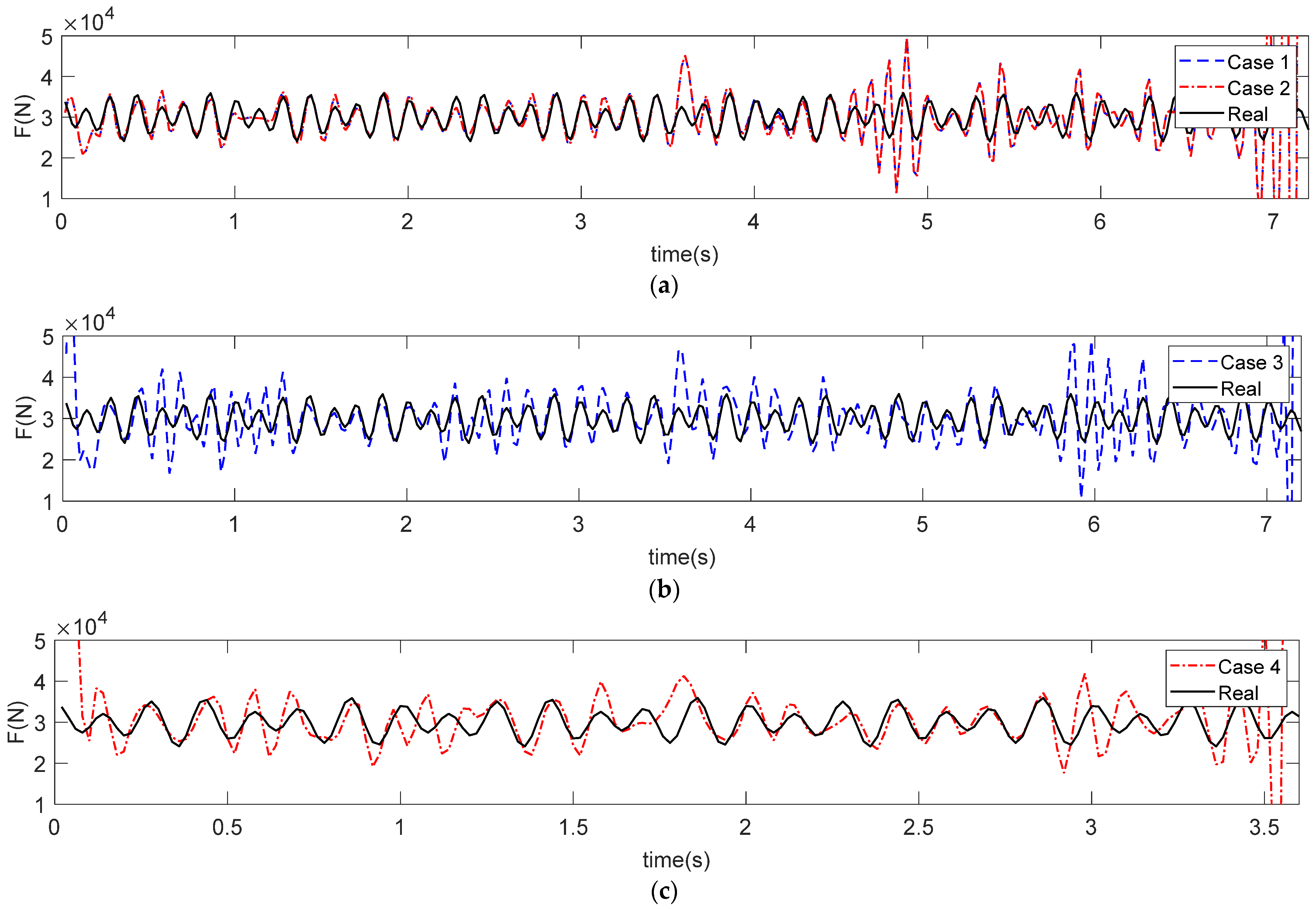
Result discussion for MFI
The moving load identification results are shown in Figure 6. The RPEs are shown in Figure 7.
  • Influence of damage severity and location
Comparing the results of Cases 1 and 2 in Figure 6a, it is apparent that the change of damage severity has little effect on the determined accuracy. It is because that small local damage has limited influence on the global stiffness of the bridge, so the dynamic behaviors of intact and damaged are similar. This minor difference is optimized by TLSF and hence does not affect the results. On the other hand, local interference is observed at the damage location. Visible increase is found around 3.6 s when the force passes Damage 1. A similar situation is also found in Cases 5 and 6 (Figure 6d,e). The results show large variation when the forces move through Damage 2, which proves that the damage changes the local stiffness.
  • Effects of force speed and number
In Cases 3, 4, and 6, the effects of load velocity and number are studied. It can be seen from Figure 6b,c that the change of velocity does not greatly influence the identification precision. The RPEs in Figure 7 also agree that both cases are determined with good accuracy. It is worth noting that significant error occurs at the beginning and end of the time period; it is a typical problem in MFI caused by the vibration instability when the load enters or exits the bridge [30].
When 2-axle forces are applied in Cases 5 and 6, a distinct error is discovered at the wave crest; phase difference is also partially found in the curve. This is mainly due to the similarity of the forces, namely the value, frequency, and, especially, their close position. The bridge–force interactions generated by these forces interfere each other and make the forces difficult to be distinguished by the method. This influence is also enlarged by the vibration instability when the forces leave the bridge and then causes identification failure. Nevertheless, it is important to state that the error basically meet the characteristic of normal distribution, so it could be decreased by averaging. It is predictable that this method will have good performance in determining axle loads of vehicles during practical application.
  • Influence of measurement noise and sensor location
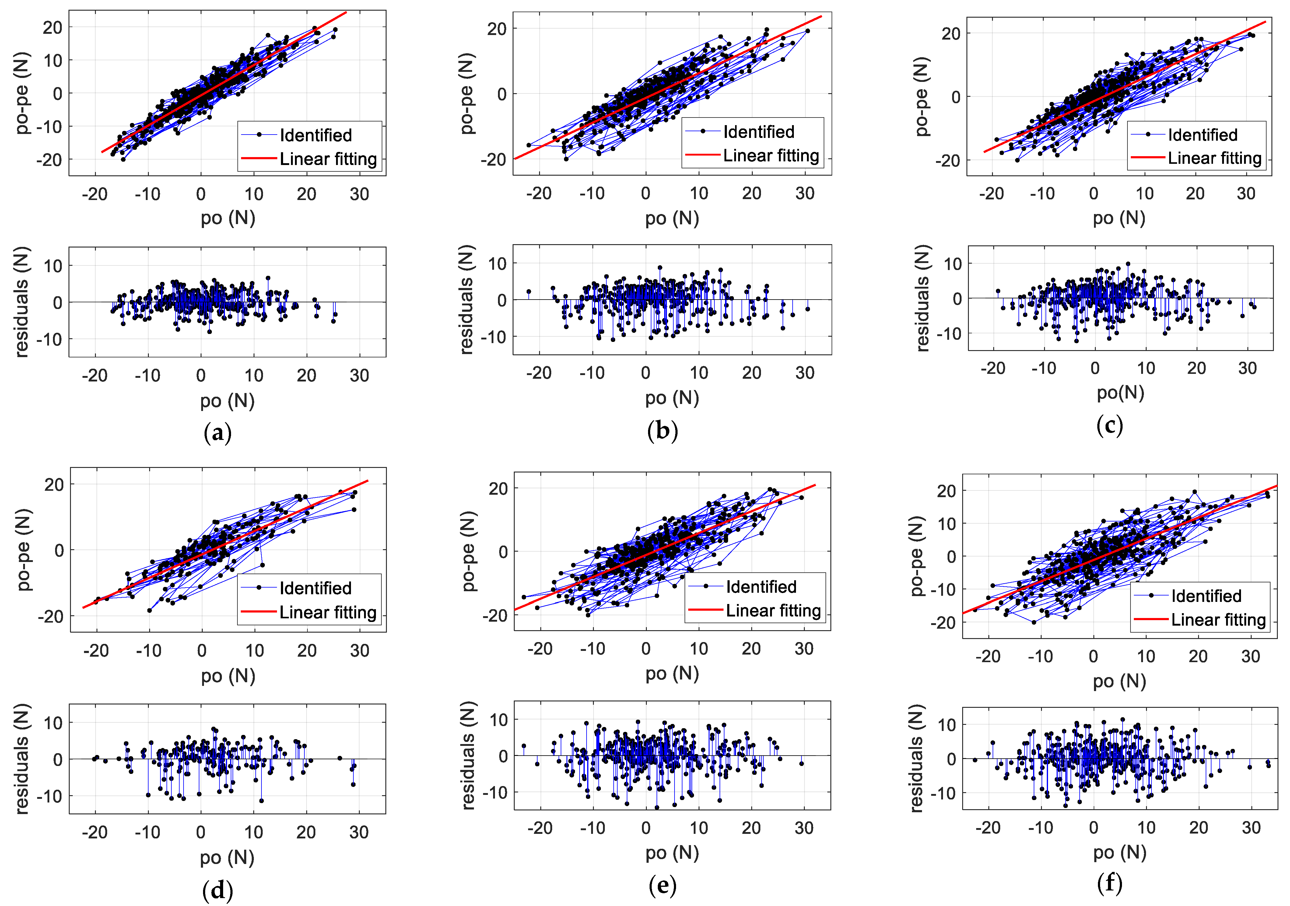
Looking into Figure 6d,e, with the growth of noise, only a slight increase of the peak values are found in the results; the frequency-phase characteristics remain unchanged. This shows good robustness of the proposed method to measure noise. Analyzing the results of Cases 2–4 (Figure 6a,b), which use different sensors, it is illustrated that forces are determined with better accuracy around the sensors. As the system matrix in the identification Equation (17), namely the TLSF response matrix Λ , is constituted of the responses excited by the small TLSFs, the details in responses captured by the sensor reduce when the TLSFs get away and hence produces a larger error. Therefore, in real-world practice, it is recommended to utilize the sensors evenly on the bridge.
(2)
Result discussion for SDI
The identified virtual force p e (equals to λ 11 e ) and calculated nodal force p o (equals to λ 11 o ) are presented in Figure 8 according to Equation (18), and the fitted damage severity 1 ζ 1 and R-squared values are listed in Table 3.
  • Influence of damage severity and measurement noise
Figure 8a,b illustrate the damage ratios determined in Cases 1 and 2. It is found that both 5% and 20% of damages are estimated. The errors are around 4%. However, if we look at the RPE, it reaches 94.6% in Case 1 while it is only 21.25% in Case 2. It deduces that the damage determination accuracy of this method is low correlated with the damage severity. It is because when the damage is transformed to external virtual force, its identification accuracy is dominated by the precision of the TLSF matrix, not the magnitude of the force itself. In this aspect, it is an advantage of this method, but it also makes the method insensitive to small damage. This drawback could be developed by introducing an appropriate objective function [31], which should be studied further.
Comparing Cases 2 and 3, the influence of measurement noise mainly reflects the confidence of the fitting curves, while the effect on results is relatively low.
  • Influence of moving force
Observing the fitted damage severity results of Cases 3 and 4, it is determined that the force-velocity has a minor effect on the SDI accuracy, which is similar to the MFI results. Conversely, the 2-axle force cases show that increasing the number of unknowns significantly impacts the precision of damage detection and the confidence of fitting. The response of a damaged structure is the superposition of an intact structure subjected to the moving force and virtual force, respectively. Therefore, the synchronized inversion of moving force and virtual force will interfere with each other. Hence the reason for the accuracy loss is not the number of moving forces, but the error produced during the method distinguishing the forces. This drawback may be improved by utilizing more sensors and optimizing the precision of the TLSF matrix.

4. Conclusions

This paper develops a synchronized assessment method on bridge structural damage and moving force. Through transforming structural damage to virtual force, this method unifies the SDI and MFI to a multi-force identification problem. Then the TLSF technique is proposed to improve the calculation efficiency and stability of the inverse problem. A continuous beam and a truss bridge are simulated as examples to validate the proposed method. The effectiveness in respect to the aspects of force type, velocity, number, as well as damage severity, location, and measurement noise are studied. The conclusions are presented as follow:
1. A harmonic force and a square wave impulse force are identified via the TLSF in the continuous beam example. Both of them are determined with good accuracy. With the enhancement of TLSF, the dimension of the system matrix has been reduced from ( 1000 × 1000 ) to ( 64 × 100 ) , which significantly improves the efficiency. In addition, the L-curves of the TLSF matrix is smooth and contains little residual even in the case of considering 5% white noise, which proves the outstanding robustness of this method to noise. However, a visible error is shown in the result calculated from the response of the right span (the force is applied on the left span). This is because the restrain of the mid-support disturbs the TLSF matrix. Therefore, the optimization of sensor arrangement should be further studied.
2. The structural damage and 2-axle moving load are synchronized and identified in the truss bridge example. For the MFI, the velocity, damage severity, sensor position, and noise only cause local interference in the results, the RPEs in these cases are kept within tolerable limits. However, in the 2-axle forces cases, the error is increased due to the interplay of bridge–force interactions. Despite this, the error obeys normal distribution, which could be reduced by a certain optimization method. In terms of SDI, results find that the accuracy is low correlated to damage severity and location but is dominated by the precision of the TLSF matrix and is interfered with the singularity generated from multi-force identification. These drawbacks could be improved by choosing appropriate objective functions and optimization algorithms.
The numerical studies prove the potential of this method in real-world application. The essential problem is to establish an accurate TLSF matrix, which makes a finite element model of the intact bridge necessary. Due to this, the method is better applied on new bridges with complete structure information and the maintenance of subsequent damages. In addition, many factors should be considered before the method is applied. The influences of road profile, multilane, and the vehicle–bridge coupling effect will be studied in the future.

Author Contributions

Conceptualization, methodology, and validation, J.Z. and Z.X.; resources and data curation, C.L.; writing, Z.X. All authors have read and agreed to the published version of the manuscript.

Funding

The authors gratefully acknowledge the support provided by the National Science Foundation of the Jiangsu Higher Education Institution of China (Grant No. 20KJD560002) and the Nantong Science and Technology Plan Project (Grant No. JC2020124).

Data Availability Statement

Data is contained within the article.

Conflicts of Interest

The authors declare no conflict of interest.

References

  1. Brouste, A. Testing the accuracy of WIM systems: Application to a B-WIM case. Measurement 2021, 185, 110068. [Google Scholar] [CrossRef]
  2. Yu, Y.; Cai, C.S.; Deng, L. Vehicle axle identification using wavelet analysis of bridge global responses. J. Vib. Control 2017, 23, 2830–2840. [Google Scholar] [CrossRef]
  3. Outay, F.; Mengash, H.A.; Adnan, M. Applications of unmanned aerial vehicle (UAV) in road safety, traffic and highway infrastructure management: Recent advances and challenges. Transp. Res. Part A Policy Pract. 2020, 141, 116–129. [Google Scholar] [CrossRef]
  4. Pitkänen, T.P.; Piri, T.; Lehtonen, A.; Peltoniemi, M. Detecting structural changes induced by Heterobasidion root rot on Scots pines using terrestrial laser scanning. For. Ecol. Manag. 2021, 492, 119239. [Google Scholar] [CrossRef]
  5. Lee, H.; Koo, B.; Chattopadhyay, A.; Neerukatti, R.K.; Liu, K.C. Damage detection technique using ultrasonic guided waves and outlier detection: Application to interface delamination diagnosis of integrated circuit package. Mech. Syst. Signal Process. 2021, 160, 107884. [Google Scholar] [CrossRef]
  6. Chan, T.H.T.; Yu, L.; Law, S.S.; Yung, T.H. Moving force identification studies, I: Theory. J. Sound Vib. 2001, 247, 59–76. [Google Scholar] [CrossRef]
  7. Law, S.S.; Chan, T.H.T.; Zhu, Q.X.; Zeng, Q.H. Regularization in Moving Force Identification. J. Eng. Mech. 2001, 127, 136–148. [Google Scholar] [CrossRef]
  8. Pan, C.D.; Yu, L.; Liu, H.L.; Chen, Z.P.; Luo, W.F.J.M.S.; Processing, S. Moving force identification based on redundant concatenated dictionary and weighted l1-norm regularization. Mech. Syst. Signal Process. 2018, 98, 32–49. [Google Scholar] [CrossRef]
  9. Ren, Y.; Cheng, W.; Wang, Y.; Wang, B. Analysis of flexural behavior of a simple supported thin beam under concentrated multiloads using trigonometric series method. Thin-Walled Struct. 2017, 120, 124–137. [Google Scholar] [CrossRef]
  10. Huang, C.; Ji, H.; Qiu, J.; Wang, L.; Wang, X. TwIST sparse regularization method using cubic B-spline dual scaling functions for impact force identification. Mech. Syst. Signal Process. 2022, 167, 108451. [Google Scholar] [CrossRef]
  11. Nguyen, T.Q.; Vuong, L.C.; Le, C.M.; Ngo, N.K.; Nguyen- Xuan, H. A data-driven approach based on wavelet analysis and deep learning for identification of multiple-cracked beam structures under moving load. Measurement 2020, 162, 107862. [Google Scholar] [CrossRef]
  12. Liu, J.; Sun, X.; Han, X.; Jiang, C.; Yu, D. A novel computational inverse technique for load identification using the shape function method of moving least square fitting. Comput. Struct. 2014, 144, 127–137. [Google Scholar] [CrossRef]
  13. Pan, C.D.; Yu, L. Moving Force Identification Based on Firefly Algorithm. J. Adv. Mater. Res. 2014, 3149, 329–333. [Google Scholar] [CrossRef]
  14. Boubaker, S. Identification of monthly municipal water demand system based on autoregressive integrated moving average model tuned by particle swarm optimization. J. Hydroinform. 2017, 19, 261–281. [Google Scholar] [CrossRef]
  15. Avci, O.; Abdeljaber, O.; Kiranyaz, S.; Hussein, M.; Gabbouj, M.; Inman, D.J. A review of vibration-based damage detection in civil structures: From traditional methods to Machine Learning and Deep Learning applications. Mech. Syst. Signal Process. 2021, 147, 107077. [Google Scholar] [CrossRef]
  16. Roy, K.; Ray-Chaudhuri, S. Fundamental mode shape and its derivatives in structural damage localization. J. Sound Vib. 2013, 332, 5584–5593. [Google Scholar] [CrossRef]
  17. Huang, M.; Li, X.; Lei, Y.; Gu, J. Structural damage identification based on modal frequency strain energy assurance criterion and flexibility using enhanced Moth-Flame optimization. Structures 2020, 28, 1119–1136. [Google Scholar] [CrossRef]
  18. Wang, Y.; Xiang, Z.; Gu, Z.; Zhu, C.; Qian, W. Damage Detection in Different Types of 3D Asymmetric Buildings Using Vibration Characteristics. Shock. Vib. 2021, 2021, 6004283. [Google Scholar] [CrossRef]
  19. Farahani, R.V.; Penumadu, D. Damage identification of a full-scale five-girder bridge using time-series analysis of vibration data. J. Eng. Struct. 2016, 115, 129–139. [Google Scholar] [CrossRef]
  20. Lee, E.-T.; Eun, H.-C.; Elahinia, M. Structural Damage Detection by Power Spectral Density Estimation Using Output-Only Measurement. J. Shock. Vib. 2016, 2016, 8761249. [Google Scholar] [CrossRef] [Green Version]
  21. Andrzej, K.; Viriato, A.d.S.J.; Hernâni, L. Damage identification by wavelet analysis of modal rotation differences. J. Struct. 2021, 30, 1–10. [Google Scholar]
  22. Minshui, H.; Wei, Z.; Jianfeng, G.; Yongzhi, L. Damage Identification of a Steel Frame Based on Integration of Time Series and Neural Network under Varying Temperatures. J. Adv. Civ. Eng. 2020, 2020, 4284381. [Google Scholar]
  23. Zhu, X.; Law, S. Damage detection in simply supported concrete bridge structure under moving vehicular loads. J. Vib. Acoust. 2007, 129, 58–65. [Google Scholar] [CrossRef]
  24. Zhang, K.; Law, S.; Duan, Z. Condition assessment of structures under unknown support excitation. Earthq. Eng. Eng. Vib. 2009, 8, 103–114. [Google Scholar] [CrossRef]
  25. Zhang, Q.; Jankowski, Ł.; Duan, Z. Simultaneous identification of moving masses and structural damage. Struct. Multidiscip. Optim. 2010, 42, 907–922. [Google Scholar] [CrossRef] [Green Version]
  26. Xiang, Z.; Chan, T.H.; Thambiratnam, D.P.; Nguyen, A. Prestress and excitation force identification in a prestressed concrete box-girder bridge. Comput. Concr. 2017, 20, 617–625. [Google Scholar]
  27. Kołakowski, P.; Wikło, M.; Holnicki-Szulc, J. The virtual distortion method—A versatile reanalysis tool for structures and systems. Struct. Multidiscip. Optim. 2008, 36, 217–234. [Google Scholar] [CrossRef]
  28. Clough, R.; Penzien, J. Dynamics of Structures, 1st ed.; McGraw-Hill Companies: New York, NY, USA, 1975; pp. 87–89. [Google Scholar]
  29. Chen, Z.; Chan, T.H.T. A truncated generalized singular value decomposition algorithm for moving force identification with ill-posed problems. J. Sound Vib. 2017, 401, 297–310. [Google Scholar] [CrossRef]
  30. Chan, T.H.T.; Yu, L.; Law, S.S.; Yung, T.H. Moving force identification studies, II: Comparative studies. J. Sound Vib. 2001, 247, 77–95. [Google Scholar] [CrossRef]
  31. Huang, M.S.; Cheng, X.; Lei, Y.Z. Structural Damage Identification Based on Substructure Method and Improved Whale Optimization Algorithm. J. Civil. Struct. Health Monit. 2021, 11, 351–380. [Google Scholar] [CrossRef]
Figure 1. Continuous beam model.
Applsci 12 00691 g001
Figure 2. Excitations and corresponding responses.
Applsci 12 00691 g002
Figure 3. L-curves of TLSF response matrix and Impulse response matrix with respect to D1 with 5% noise. (a) L-curve of Λ ; (b) L-curve of I.
Applsci 12 00691 g003
Figure 4. Fixed force identification results. (a) Harmonic force identification results; (b) Square wave force identification results.
Applsci 12 00691 g004
Figure 5. A simply supported truss beam under moving load.
Applsci 12 00691 g005
Figure 6. Moving force determination results in the synchronized assessment. (a) Cases 1 and 2; (b) Case 3; (c) Case 4; (d) Case 5; (e) Case 6.
Applsci 12 00691 g006aApplsci 12 00691 g006b
Figure 7. RPEs of moving force identification.
Applsci 12 00691 g007
Figure 8. Identified and fitted results of ζ 1 . (a) Case 1; (b) Case 2; (c) Case 3; (d) Case 4; (e) Case 5; (f) Case 6.
Applsci 12 00691 g008
Table 1. RPE of fixed periodic load identification.
RPE (%)Harmonic ForceSquare Wave Force
via D1 response1.56.72
via D1 response with 5% noise5.739.42
via D2 response−48.113.41
via D2 response with 5% noise−49.122.85
Table 2. Case setting.
Case No.Velocity (m/s)Damage SeverityDamage LocationForce No.Noise LevelUsed Sensor
1105%Damage 1F15%S1 and S2
220%
31020%Damage 1F110%S1 and S3
420S2 and S3
51020%Damage 2F1 and F25%S1, S2 and S3
610%
Table 3. Fitted damage severity 1 ζ 1 and R-squared value.
Case No.Damage SeverityR-Squared ValueCase No.Damage SeverityR-Squared Value
19.73%0.8692428.72%0.7556
224.25%0.7938530.96%0.6723
325.83%0.7429634.28%0.6311
Publisher’s Note: MDPI stays neutral with regard to jurisdictional claims in published maps and institutional affiliations.

