Abstract
We consider the use of remote sensing for large-scale monitoring of agricultural land use, focusing on classification of tillage and vegetation cover for individual field parcels across large spatial areas. From the perspective of remote sensing and modelling, field parcels are challenging as objects of interest due to highly varying shape and size but relatively uniform pixel content and texture. To model such areas we need representations that can be reliably estimated already for small parcels and that are invariant to the size of the parcel. We propose representing the parcels using density estimates of remote imaging pixels and provide a computational pipeline that combines the representation with arbitrary supervised learning algorithms, while allowing easy integration of multiple imaging sources. We demonstrate the method in the task of the automatic monitoring of autumn tillage method and vegetation cover of Finnish crop fields, based on the integrated analysis of intensity of Synthetic Aperture Radar (SAR) polarity bands of the Sentinel-1 satellite and spectral indices calculated from Sentinel-2 multispectral image data. We use a collection of 127,757 field parcels monitored in April 2018 and annotated to six tillage method and vegetation cover classes, reaching 70% classification accuracy for test parcels when using both SAR and multispectral data. Besides this task, the method could also directly be applied for other agricultural monitoring tasks, such as crop yield prediction.
1. Introduction
Remote sensing offers a cost-efficient approach for large-scale agricultural land use monitoring for administrative and research purposes, especially when combined with machine learning (ML) methods for estimating land use characteristics for individual crop field parcels [1,2,3] or other small spatial regions. These methods require a representation for each parcel derived from its pixels, either an explicitly engineered collection of features or an internal representation learnt in a data-driven fashion as in popular deep learning methods such as Convolutional Neural Networks (CNN) [4,5,6,7]. Our work is about learning good representations for crop field parcels that are often small and vary in shape. We also provide a practical computational pipeline for large-scale agricultural monitoring that can efficiently integrate information provided by multiple raster images captured at different resolutions, demonstrating it for the case of off-season soil tillage monitoring in Finland.
Previous studies have indicated object-level classification to be preferable over pixel-level information in agricultural tasks [8,9], but typically very high-level aggregate information such as the mean of individual pixel values has been used for representing parcels, making discrimination between similar classes difficult. Even though spatial features as extracted by CNNs are nowadays routinely used in remote sensing, crop field parcels have several characteristics that motivate representations focusing on the spectral distribution of sensor values instead. First of all, image content within each parcel is nearly homogeneous since the parcels are managed in a uniform way within the parcel boundaries. Hence, the prior value of spatial information at the pixel level is low. Spatial statistics are also difficult to estimate for parcels of irregular shape and with large differences in size, especially for noisy imaging sources like Synthetic Aperture Radar (SAR) as well as for cloud-occluded multispectral images (MSI). Distributional information about sensor values can, however, be reliably estimated for objects of any size and shape also in the presence of occlusion and noise. Consequently, we propose using probability density estimates (DE) of pixel values as a general purpose representation for such objects and formalize a practical computational pipeline around these representations, described in Section 2.2.
We assume the pixels of a given raster image area to be drawn from a probability distribution of pixel band values. Rough aggregate summaries, such as mean and median of the pixel values are still in active use in remote sensing due to simplicity and robustness [10,11,12,13], but our interest lies in the advantages of characterising subtle differences in the whole distribution. Histograms of pixel values have a long history as a natural representation of spectral distribution in computer vision [14,15,16], and they have also been considered in remote sensing [17,18,19]. Normalized object histograms are easy to compute but suffer from poor sample efficiency and objects with different pixel counts are not directly comparable: a small object’s histogram is likely to have gaps whereas larger ones appear to be more continuous. Hence, histograms work best at a coarse bin resolution. We prefer direct modelling of the joint density using multivariate DEs [20,21], so that for each object we learn a continuous probability density over multi-band pixel values. To use the estimate as representation for subsequent processing, we collapse the density to bins resemblant of a histogram, with the advantage of inter- and extrapolation over observation gaps and reduced noise in pixel values, especially for parcels of varying size. We also consider Bayesian estimators [22] to account for uncertainty stemming from small pixel counts; in our data the field parcel size varies from tens to hundreds of pixels.
We apply the proposed method to a case of off-season soil tillage monitoring in Finland. From the standpoint of environmentally and economically sustainable agriculture, soil erosion and nutrient runoff from crop fields to surface waters is a long-standing challenge, to which soil tillage operations are a contributing factor [23,24]. Large-scale information on annual off-season tillage status of arable land is of interest for agro-environmental monitoring administration, policy makers as well as wide range of academic domains from terrestrial carbon studies to hydrological research. The problem is made challenging by the irregular shapes and small sizes of the parcels in Finland, and the limited amount of labeled training data within a single country. Furthermore, the annual off-season observation time window is limited and must take place during a relatively cloudy time of the year in Finland. The proposed computational pipeline can address all of these challenges.
Previous remote sensing studies of soil tillage detection have focused on spectral reflectance characteristics [25,26,27] or radar response [28,29,30] of soils, green vegetation, and crop residues. SAR signal penetrates cloud cover and is inherently sensitive to target 3D structure affecting backscatter mechanisms and angle. On the other hand, optical, for example. multispectral reflectance from satellite images can be fully exploited only at cloudless moments, but it can characterize a wide range of chemical and physical properties of matter as well as reveal dynamics of organic phenomena. The differences in the physical processes involved in radar backscatter and optical reflectance signals allow them to respond complementarily to the phenomena being interpreted, which results in enhanced accuracy of classification and regression for a range of remote sensing applications, for example, in agricultural or land cover contexts [31,32,33,34,35], or recently in soil tillage detection [36,37]. Our contribution to the topic is a practical, effort-reducing SAR-MSI data fusion technique. We use Copernicus Sentinel-1 (S1) SAR data with dimensions of two polarity bands, overlaid with polygon data of crop fields as provided by the Finnish Food Authority. Similarly to SAR bands, we construct density estimates over two spectral indices calculated from a Sentinel-2 (S2) MSI for the same fields during a suitably narrow time window. Both sources are then merged to estimate the soil tillage category. Besides the Sentinel data used here, we expect the approach to be applicable to other SAR and MSI data sources, such as Radarsat-2, Landsat, or Modis.
To summarize, as the main contributions of this work we:
- Present a method for off-season tillage and vegetation cover detection on crop field parcels, which is a challenging task due to the heterogeneous size of the objects and a limited amount of training observations;
- Propose a representation of a free-form raster image object as a non-parametric probability density estimate, to be used for increasing robustness to variability in object size, count and missing pixel data;
- Introduce an easy-to-use framework for multi-sensor raster data fusion for sources of varying spatial resolution, applicable also outside the specific task considered here.
2. Materials and Methods
2.1. Materials
We use polygon-delineated boundaries of Finnish crop field parcels illustrated in Figure 1, collocated with mosaics of SAR and MSI satellite images over a time period from 11–23 April 2018 from Copernicus Sentinel-1 and Sentinel-2 missions, where the parcels are classified to one of multiple crop field tillage operations that affect, for example, soil properties and nutrient runoff to surface waters. The illustration reveals that the parcels have complex shapes and varying sizes, and that many of the parcels are small.
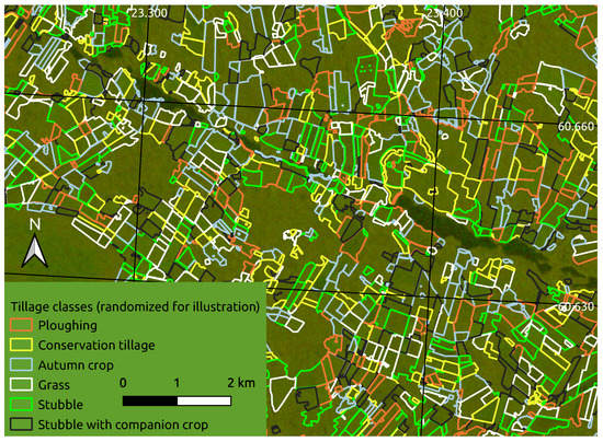
Figure 1.
Foreground polygons: Autumn tillage operations annotated to six classes (colors). Background raster: Red-green rendering of a VH+VV dual polarization Sentinel-1 SAR image. Note: Due to data protection regulations, the polygons are from publicly open similar data from 2016 instead of our actual data, and the classes are randomized.
2.1.1. Crop Field Parcels and Annotations
We are interested in six categories to gauge the variety of land use and management over winter. The first class of conventional ploughing means mould-board ploughing in autumn to a depth of 20–25 cm. The second class of conservation tillage comprises tilling methods that mechanically disturb the soil to a depth less than 15 cm while retaining most of the crop residues on the surface. The last four classes include cases where the soil is either covered with crop residues (stubble), or with vegetation (autumn crop, grass). Soil with autumn crop has typically sparse plant cover before the growing season, and the soil surface is rough after seedbed preparation, whereas grass vegetation is typically rather thick, and the soil is covered. Stubble fields are covered with stalks and crop residues. In autumn spontaneous regrowth and weeds typically start to re-vegetate the soil. A special category of stubble field growing catch crops means crop fields where a companion crop (catch crop) re-vegetates the soil after the harvest of the main crop.
The region of interest (ROI) is illustrated in Figure 2 and was chosen on agrometeorological grounds: autumn tillage operations can span over many autumn months depending on the soil moisture conditions up until the soil is frozen and covered with snow. Therefore, the optimal time window to acquire images to monitor winter-time tillage status is shortly after snowmelt and before seedbed preparation in the spring. This time window is typically quite short; from two to four weeks. During this time, the soil dries out fast, but also there may occur sudden snow showers. To select the ROI, we used the regional starting dates of the thermal growing season in 2018. In this region, by mid April, the mean daily temperature permanently exceeded 5 °C, and snow had melted from open areas. The ROI was used to mask the underlying field parcels for reference data.
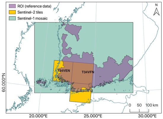
Figure 2.
The region of interest (ROI) and raster data extent over southern Finland.
Reference data were annotated as follows. Information on agricultural land use in agricultural registers from two preceding growing seasons—2017 and 2018—were compared. The soil cover class was decided based on the variables of the winter-time vegetation cover related parcel-wise agri-environmental measures declared by farmers. Conservation tillage and vegetation cover are subsidised and subscribed to parcels. The different types of vegetation and crop residue cover were inferred from comparing the preceding years crop types with expertise in crop management. If a parcel was not subscribed to any measure, it was considered ploughed.
The intersection of the area of the satellite images shown in Figure 2 and of the parcel polygons yields a total of 127,757 annotated parcels. Annotations across the six classes are distributed as follows:
Conventional tillage, that is, ploughing 46,765; Conservation tillage 15,211; Autumn crop 2681; Grass 24,503; Stubble with no tillage 37,750; and Stubble with companion crop 847. We assigned each parcel exclusively to training and test sets by random sampling in a proportion of 80% for training and 20% for testing, resulting in total of 102,206 samples available for training and 25,551 for testing. However, in the computational experiments we mostly used considerably smaller subsets for studying the accuracy of models trained on less data.
2.1.2. Satellite Imagery
As the first raster component, we use polarimetric SAR intensity data (Ground Range Detected, GRD) from the Copernicus Sentinel-1 mission. Due to highly dynamic soil moisture and even plausible short-lived snow cover conditions during the time window, it is advantageous to use a mean-valued mosaic image composed of several images over the time period. The Finnish Meteorological Institute (FMI) publishes a preprocessed 11-day Sentinel-1 mean gamma-nought mosaic product [38]. See Supplement S1 for additional information and availability of the mosaic. We use an instance of a VV and VH polarity dataset from April 2018 (11th to 21st). Although the underlying spatial resolution of a Sentinel-1 Interferometric Wide Swath image is 5 × 20 m for an image of a 250 km swath [39], FMI mosaic preprocessing [38] resamples the data to 20 m spatial resolution. As a restriction, measurements prior to 2019 were quantized to 1 dB intensity intervals by the FMI data pipeline, posing a hard limit to discretization, that is, the binning of the measurements for the density estimators. Individual Sentinel-1 images that coincide with the time period and location of the mosaic and our ROI are listed in Supplement S1.
As a second raster component, we spatially mosaic three Sentinel-2 multispectral images selected from as close to the time period and ROI of the Sentinel-1 mosaic as possible (see Supplement S2 for the image identifiers), resampled to 10 m spatial resolution. An additional criterion for this image selection was a relatively low overall (<10%) percentage of pixels containing cloud or snow in the quality indicator (QI) metadata of the images. We also filter out individual pixels with a cloud or snow confidence value of ≥10%. This reduces the amount of pixel observations per parcel and makes the pixel sets discontinuous, but these properties do not cause problems for the proposed approach.
From the Sentinel-2 spectral channels, we calculate relevant basic spectral indices—the Normalized Differential Vegetation Index () [40] and Normalized Differential Tillage Index () [41,42]—as features for our density estimates. Consequently, we have for MSI images. The formulas for the indices in the context of Sentinel-2 bands are:
and
where the Sentinel-2 band center wavelengths are: (Red): 670 nm, (NIR): 830 nm, (SWIR): 1610 nm, and (SWIR): 2200 nm.
The SAR VH/VV bands and the two optical spectral indices per pixel represent two disparate data sources at different resolutions and image extents (as seen in Figure 2). In Section 2.2 below we combine these to a common representation per parcel by extracting the pixels that coincide with the parcel delineation polygons.
2.2. Methods
2.2.1. Problem Formulation
The agricultural land monitoring task can be formulated as a machine learning problem, where we learn to predict a label for a previously unseen object (field parcel) given a collection of training observations . For notational simplicity, we present the details for classification problems (y are discrete and mutually exclusive categories) although the representation could also be used for regression (continuous y, such as crop yield) or structured output problems.
Our focus here is on learning a suitable representation for objects that are pixel subsets of raster images. We denote individual pixels by column vectors where the individual elements correspond to different channels (e.g., spectral bands of MSI or polarization channels of SAR). Each object o is defined by some subset of the pixels of an image captured within a geospatial region of interest A, and hence can be represented by a matrix storing the pixels for this object as its columns. Note that this formulation can be generalized in various ways; see Section 4.2.
Even though the focus of this work is on SAR and MSI data for soil tillage applications, we note that the approach is applicable to any task that satisfies the requirements of: (1) multi-banded raster data on a region of interest; (2) objects defined in terms of pixel segments of the images with a (3) class annotation on each object, using a shared coordinate reference system between the segment annotations and the rasters.
2.2.2. Data Flow: From Objects to Representations and Classification
Figure 3 shows a full data flow from raw images to predictions for the case of two remote sensing image sources. After sensor- and application-specific preprocessing and pixel-wise feature engineering of the images , we extract for each object these resulting pixels from each type of image. We associate with each object an unordered pixel set per image type from within the geometric boundaries of the object shape. In the following, we represent these data from two data sources of different resolutions and extents using a shared representation of a multidimensional probability distribution per parcel.
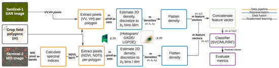
Figure 3.
Process diagram with data flow from left to right.
From the object-wise pixel sets we form density estimates for each object separately using a selected density estimation method, and then evaluate the density along a regular grid G to form the representation . For practical computation, this representation is formatted as a vector, which we normalize for additional robustness so that the norm is one, but this normalization is not a critical part of the pipeline. This vector then becomes the representation for the supervised learning algorithm. For Bayesian density estimators, we can also consider an alternative representation that also captures the uncertainty of the estimate, explained later after describing the Logistic Gaussian Process Density Estimation (LGPDE) method.
Since our main focus is on the representation itself, we use standard classifiers readily available as a program library and in frequent use in the research field: the scikit-learn library’s implementation of the Random Forest (RF), Support Vector Machine classifier (SVC) and a shallow feed-forward neural network (Multi-Layer Perceptron; MLP).
2.2.3. Density Estimate as a Representation
A desirable object representation should condense relevant information into a similar form whether the object is spatially small or large. Put more generally, objects should be commensurately represented for an arbitrary count of observations in the measurement space. All density estimates and normalized histograms formally fulfill this requirement and we can use them to represent the object, but as discussed next, practical methods differ in terms of comparability given different amounts of pixels.
We consider a fixed-dimensional representation suitable as an input for any classifier, where the are center points of elements (bins) in an equally spaced grid G overlaid on the density’s support dimensions (pixel bands), so that G has B discretization intervals in each of the D dimensions, with a total of elements. is a probability density that we learn based on the object’s pixel collection X and then evaluate the density at the points of G to form the representation. We consider only cases with , where the channels are two SAR polarisations or the two vegetation indices for MSI, so that we can directly model the joint density. For higher-dimensional cases, an alternative approach is to estimate a marginal density for each channel separately and evaluate it along a grid of B elements, resulting in a representation for each band separately. A combined representation can then be obtained by concatenating these as .
The representation can be computed for all density estimators, and next we discuss three practical alternatives and their properties.
Multivariate Histogram
As the elementary density estimate, we consider the multivariate histogram. For common notation with the other estimators, we formulate the normalized multivariate density histogram in the style of the univariate definition in [21] as a discretized function over G and multivariate observations with a total count of n:
where is the number of observations falling into the multivariate interval whose index is denoted by g. These intervals are defined as symmetric hybercubes around the center points of the grid.
Histograms are broadly used as representations, but are problematic for small objects with few pixels. We either need to use very small B, losing most of the resolution, or accept that the bin estimates are increasingly noisy. For large B we will typically have a significant proportion of bins with no observations at all and the non-zero bins will include only one pixel observation, and this effect becomes more severe with large D. If the pixel observations have noise comparable to or larger than the bin width , a pixel often falls into one of the neighboring bins (or even further), and direct comparison of two histograms computed for two noisy realizations of the same object would indicate no similarity. Histograms also ignore uncertainty completely, which makes them poorly suited for the comparison of objects of varying size; histograms estimated from fewer pixels are noisier but this information is not captured by the estimate, and subsequent learning algorithms would falsely attribute the same amount of confidence for both.
Kernel Density Estimation
Parzen [43] formulated univariate kernel density estimation (KDE) in its modern form including the smoothing parameter, that is, bandwidth h, as:
where the kernel K is a non-negative function and are the n data points. We use an analogously defined multivariate version of KDE [20,44] with a bandwidth matrix as:
with the standard Gaussian kernel and a diagonal bandwidth matrix as the covariance matrix determined by Scott’s rule [21]. Note that for small objects the estimator is smoothed more, due to an inverse relationship between n and . We refer to this estimate as Gaussian KDE (GKDE).
GKDE is an effective, lightweight method of providing smoothed probability density estimates for point samples independently of discretization interval or data point count. However, GKDE provides no measure of uncertainty relative to its suggested point estimate, and hence, similarly to histograms, loses information about the relative reliability of different objects.
Logistic Gaussian Process Density Estimation
For objects with only a few pixels, it becomes important to explicitly quantify the uncertainty of the density estimate itself, which neither of the above methods can achieve. For instance, for the extreme case of just one pixel, the histogram becomes a delta distribution, and while GKDE provides a smoother estimate it still suggests this single noisy pixel alone to be highly informative of the content. Bayesian estimators, instead, have the ability to explicitly model uncertainty, and in the following we describe one practical alternative building on Gaussian Processes (GP).
LGPDE, originally proposed by Leonard et al. [45], assigns a GP prior for the unnormalized logarithmic density so that for any , where C is a constant required for normalizing the density. The GP assigns a prior over the functions directly, so that for any finite collection of inputs their joint distribution is a multivariate normal, and conditioning on some pixel observations X we can then obtain the posterior distribution that captures the uncertainty of the estimator. Due to the logistic transform, there is no closed-form analytic expression for the posterior, but both Markov Chain Monte Carlo (MCMC) sampling [46] and Laplace approximation [22] can be used for inference. We will later evaluate both the Laplace approximation as well as an MCMC implementation using the No-U-Turn Hamiltonian Monte Carlo algorithm as provided in the Stan probabilistic programming environment [47].
We use the formulation of Riihimäki et al. [22] with explicit enumeration over discretized support axes for computing the normalization term C. A prior term results from the logistic transform:
where is a latent function representing the density estimate surface being evaluated at points of the discretization grid G, denotes the hyperparameters of the prior and the GP kernel, and is a basis function that modulates the density to achieve finite support. For 2D densities we use the basis function . For a weakly informative prior, we parametrize a covariance adjustment of and a zero mean of . The kernel determines a covariance matrix based on a given covariance function and a chosen multivariate bin discretization expressed by G. The posterior is formed using the likelihood
where is a histogram-like vector of observation counts. In the multidimensional case, and are vectorized to a single vector with elements. The model induces a density over arbitrary , but the construction is already in a form explicitly represented over the grid G. Hence the representation is formed simply as the exponent of the log density.
Rather than a fixed representation , we now have a set of S posterior samples , either as produced by the MCMC algorithm or obtained by sampling from the Laplace approximation. They can be used within the proposed pipeline in two ways. The simplest alternative is to collapse the posterior to a point estimate as , to be used similarly as the results of other estimators. We call this Point Estimate Classification (PE-C). The other alternative, here called Posterior Predictive Classification (PP-C), is to pass all posterior samples of separately to the classifier, for each object being classified. For testing, we evaluate the classifier similarly for all posterior samples and compute the posterior predictive class distribution using standard Monte Carlo approximation. This allows an end-to-end probabilistic approach for classification even if the classifier itself is designed to only produce point predictions .
3. Results
We report results for two types of experiments: Technical experiments validating the computational pipeline (Section 3.1), and evaluation of the method for the soil tillage task (Section 3.2).
3.1. Technical Validation
The core assumptions of our method are that a probability density of pixel values represents useful information about the classes of interest, and that we can learn reliable estimates of those based on individual parcels. We first validate these visually in Figure 4 for the SAR data. The top row shows that estimates computed from all pixels of a given class are visually distinct, whereas the bottom row shows that estimates computed based on pixels of individual parcels resemble the class-level information. The figure also illustrates the difficulty of the problem; the densities are distinct but highly similar in the sense that simpler representations like mean pixel value are unlikely to be sufficient for separating the classes.
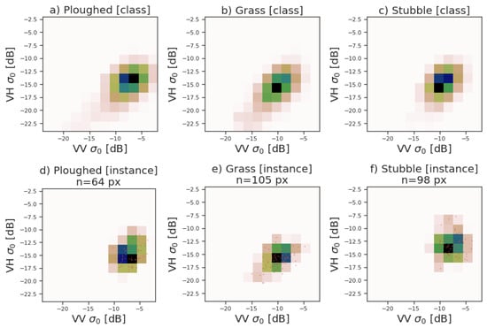
Figure 4.
Gaussian kernel density estimate representations of polarimetric SAR intensity measurements for ploughed, grass- and stubble-covered fields. (a–c): Class-level density estimates from a large random sample of all pixels of all field parcels of a class. (d–f): Density estimates for single parcels of each class. The small red dots indicate individual pixels, with small jitter so multiple pixels with identical values are also visible.
For accuracy evaluation between the method variants, we use balanced subsets of parcel data described in Section 2.1.1 to make the results easier to interpret. We consider only balanced classification problems with equally many observations for each class so that classification accuracy can directly be interpreted as quality of the method, and we only consider the classes ploughed, grass and stubble to avoid issues with classification of the three minor classes that are difficult to separate from each other. For all of the technical experiments we use a fixed randomly chosen subset of 300 parcels per class (900 samples in total) for testing, whereas the size of the used subset of training data is a parameter for many of the experiments, seen on the horizontal axis as “Number of training samples/class”. This is to investigate model performance with respect to data size.
3.1.1. Comparison of Representations
To demonstrate the effect of object representation on classifier accuracy, we compare three computationally efficient representations for three classifiers in Figure 5. The experiment was done on MSI data with NDVI and NDTI indices as image bands on data consisting of relatively small parcels (20...50 px) with bins per band. The parameter B controls both the amount of information we can capture and the reliability of the estimate; with small B the estimation task is easy but a majority of discriminative information is lost, whereas with large B we retain all information but can no longer reliably estimate the density from small samples. The choice of (resulting in 2500 bins in total) is motivated by Figure 6a, which shows the accuracy as a function of the discretization level for the case of 50 training samples per class.
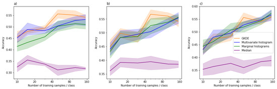
Figure 5.
Density estimates, histograms and the median as representations for multispectral NDVI/NDTI data across three different classifiers. (a) SVC (b) MLP (c) RF. Each color corresponds to a representation, the line indicates the average over five random training sets evaluated on a single test set, and the shaded areas represent 95% bootstrapping-based confidence intervals.
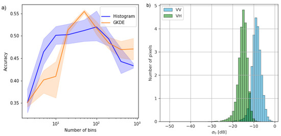
Figure 6.
Choice of the discretization bins. (a) Accuracy as function of the number of bins for S2 MSI data. (b) S1 SAR intensity (sigma nought, ) in crop field pixels concentrate within bounds of −30...0 dB.
Figure 5 reports the accuracy for varying sizes of training data for three different classifiers. The main observations for our MSI dataset are: (i) All forms of density estimates outperform naive summary statistics. The baseline of using an aggregate summary of all pixels, the median of NDVI and NDTI values, barely beats the random baseline of 33% classification accuracy, whereas all density estimates achieve accuracies between 40% and 60% depending on the case; (ii) direct multivariate estimates are at least as good as histograms and for some cases (SVC) better; (iii) GKDE performs as well as the multivariate histogram and sometimes (SVC and MLP for some training set sizes) marginally better. In summary, the results show that proper density estimators were preferable over both multivariate and marginal histograms as general representations. Even though there was no clear difference for one of the classifiers (RF), there were no cases where using GKDE would hurt.
3.1.2. Effects of Object Size
Next, we detail the performance of density-based representations under challenging training conditions with very few training instances, highly varying object size, or both. We do this on SAR data, using bins over the range dB, to keep computational complexity manageable for extensive experimentation on all estimators.
We compare three proper density estimators, GKDE and LGPDE, with two inference algorithms (MCMC and Laplace approximation) and restrict to a single choice of the classifier to streamline the results; the observations are similar for the other classifiers. Figure 7 shows the accuracies for these estimators as function of the size of the training data for three scenarios: small parcels that only uses parcels of pixels for training and evaluation, large parcels that only uses parcels of pixels for training and evalution, and variable parcels that uses both small and larger parcels (range of px). The main results are: (i) The problem is considerably easier if the objects are larger but already for the small parcels of only tens of pixels we comfortably beat the random baseline; (ii) The accuracy naturally improves when we get more training instances, but already relatively small number of approximately 30 parcels per class is enough for good accuracy; (iii) The representations are robust over parcels of varying size, shown by relatively high accuracy for the case that contains both small and large parcels; (iv) There are no clear differences between the three density estimators in terms of accuracy.
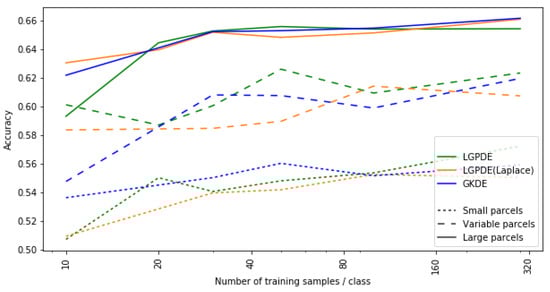
Figure 7.
Effect of field parcel size (line style) on MLP accuracy for different estimators (line color). Confidence intervals omitted for visual clarity.
Even though we did not observe a direct improvement in classification accuracy for the more advanced density estimator LGPDE, it has the advantage of explicitly modeling the uncertainty of the estimate and we can propagate it through the classification process for any classifier as explained in Section 2.2.2. To demonstrate this, Figure 8 shows the classification accuracy for the three different classifiers for a dataset of small parcels ( px), for both PE-C and PP-C. We observe that the PP-C approach that models the uncertainty offers a small but consistent improvement. Figure 9 shows that the resulting class probability distributions behave as expected—for small fields the uncertainty is better captured in the final class distributions.
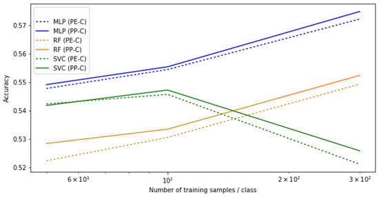
Figure 8.
Accuracy for smaller parcels increases using posterior predictive LGPDE classification.
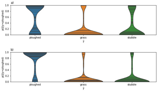
Figure 9.
Confidence of small (a) vs. large (b) ploughed fields being classified as ploughed from a probabilistic perspective, with higher uncertainty for small fields, as expected.
3.1.3. Data Fusion
By learning separate representations for each image modality (capture method or sensor) , we can perform easy data integration by simply concatenating the representations . In experiments Section 3.1.1 and Section 3.1.2 we showed that both MSI and SAR are valuable sources of information for this task, and Figure 10 shows that by further combining them we get a significant improvement in overall accuracy: The combined solution outperforms MSI, which has the higher accuracy of the single-source capturing methods, on average by approximately 8 percentage points. We show the results on 1500 test parcels for the MLP classifier; the other classifiers followed a similar pattern.
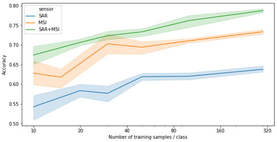
Figure 10.
Data integration vs single-source classification on a Random Forest classifier. The integrated solution clearly outperforms both MSI and SAR alone for all training set sizes.
We also evaluated the final accuracy of the data fusion solution for even larger training data to provide a baseline with ample data. With 6500 training parcels per class we reached an accuracy of 82%, validating that the accuracy can be further improved by utilising more data, as expected. However, the improvement over the 78% accuracy obtained already with 160 parcels per class is only modest. On one hand, this implies that the method can be reliably estimated already from small data and does not require access to thousands of or tens of thousands of training instances. On the other hand, it suggests the problem itself is challenging; as shown in Figure 4 and discussed in the next section, some of the classes are highly similar in appearance, which sets natural upper bounds on classification accuracy.
3.2. Soil Tillage Detection
Based on the technical validations above, we made the following choices for solving the soil tillage classification problem: (a) We use both SAR and MSI images; (b) we use RF as the classifier observed to be the most robust one; and (c) we use GKDE as computationally efficient and accurate representation. We use for MSI and B = 30 for SAR within the range of dB in alignment with [48,49,50]. Motivation for these choices is illustrated in Figure 6.
We now use all six classes described in Section 2.1.1: ploughed, conservation tillage, autumn crop, grass, stubble and stubble with companion crop. We train the model in total on 43,299 parcels with the number of samples per class ranging from 169 to 15,885, and evaluate the accuracy on 10,666 parcels not used for training. Together these form the full set of parcels we find at the intersecting area of the SAR and MSI images in our data. The overall classification accuracy, evaluated on the test parcels, was 70% and Figure 11 shows the confusion matrix for the test parcels. The largest classes ploughed, grass and stubble are classified with high accuracy, whereas the smaller classes conservation tillage, autumn crop and stubble with companion crop are more difficult to classify correctly.
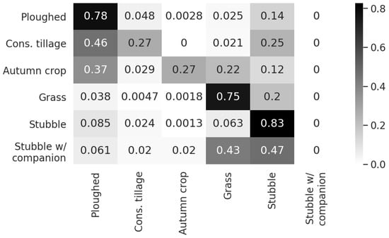
Figure 11.
Normalized confusion matrix for classification of fused SAR + MSI image objects for the full set of annotated classes.
4. Discussion
4.1. Soil Tillage Detection
Our main goal was detecting autumn tillage and vegetation cover from earth observations for large-scale agricultural monitoring. Several previous studies such as [26,28,36] on tillage detection with SAR imagery alone or fusion of SAR and MSI have concentrated on tillage intensity classification. However, few studies have detected off-season land cover classes on broader scale including also vegetation covered land cover types [37,51,52]. Shortage of studies on higher granularity of winter-time land cover classes indicates that the task is difficult.
We observed significant and consistent improvement in classification accuracy by combining SAR and MSI data. The result is well in line with those obtained both in crop tillage classification [36,37] as well as in other EO tasks [34,48,53,54,55]. Since data fusion is easy with the proposed object representations, only requiring georeferencing and simple early fusion, we strongly recommend routinely using both sources for this task. When using a single image capture method, MSI was here clearly more accurate than SAR, but this observation needs to be interpreted with care because our experiment was carried out on images with at most 10% occlusion. During a normal year, the time window for making observations on tillage operations is short and typically cloudy across Southern Finland, and MSI alone could not be trusted.
Somewhat low classification accuracy for the classes conservation tillage, autumn crop and stubble with companion crop is explained by three main reasons: (a) the amount of data for these classes is smaller compared to the other three, (b) under certain conditions some of the classes are virtually indistinguishable, and (c) the ground truth data is imperfect due to mislabeling. Regarding the difficulty of the problem, the autumn crop, stubble and stubble with companion crop all have variable amounts of plant growth that makes the classes highly similar in terms of all EO sources. Also, ploughed and conservation tillage may resemble each other after snow melt in April on certain soil types, especially where stalks have been highly decomposed.
Regarding mislabeling, the reference data were prepared with automatic rule-based labeling, which is inherently error-prone. Whereas contradictory examples (duplicates) can be removed, mislabeling remains a practical challenge due to inevitable simplifications when building the rules. Imperfections in the underlying information on agricultural practices imply that each class membership has different reliability. For example, planting of autumn crop is explicitly declared by the farmer, thus having really high reliability, whereas ploughing is merely inferred by applying a long classifying set of rules to the information. Conservation tillage is an example of low reliability. Farmers explicitly declare to apply conservation tillage in October as it is subsidized, but if weather conditions are not suitable for tilling after the declaration date, fields may remain covered by vegetation. As vegetation cover is considered the more sustainable option, “no-till” is not subject to a penalty. As a result, probability of stubble field samples mislabeled as conservation tillage is high.
For improving the quality of the reference data, one could consider unsupervised clustering techniques as in [56] to discover structure and compare with supervised techniques and the assumed labels. During data exploration we performed an initial trial with spectral and K-nearest neighbor clustering on the density representation of the objects, the results of which did suggest some internal structure within the given classes of the dataset. Additionally, specific geospatial properties such as latitude can be significant in Finland with varying microclimates affecting vegetation cover and could be used as additional features to improve the accuracy.
4.2. Modelling Aspects
The proposed computational method is applicable also for other agricultural monitoring tasks besides the specific task of tillage and vegetation cover classification, such as crop yield prediction. Furthermore, it can be applied to object-based remote sensing tasks also beyond agricultural monitoring. Hence, we also provide a brief discussion of the method itself. All forms of multivariate density estimates were observed to outperform simple object representations of aggregate summaries and marginal histograms for supervised classification of small and variably sized objects, even though the latter are easier to estimate. Proper density estimators outperformed multivariate histograms in some cases, but not in all and the difference was in general unexpectedly small. We believe this is primarily because evaluation is extremely noisy for the scenarios (the smallest datasets with the smallest objects) that would most benefit from smoothing and uncertainty quantification; more direct measures of representation quality could be considered for stronger conclusions.
Regarding the representations, GKDE [57,58] has only negligible computational overhead compared to histograms and no additional tuning parameters (due to the automatic rule for selecting the bandwidths ), and hence works as general plug-in replacement for histograms—we did not observe any reasons to prefer using histograms over GKDE. LGPDE [22] was demonstrated to further slightly improve accuracy while facilitating uncertainty propagation for arbitrary classifiers, but this comes with a significant computational overhead, even when using the more efficient Laplace approximation. Our results indicate that there is value in explicitly modeling the uncertainty of the density estimate itself but we do not yet provide a practical approach for arbitrary problems; to proceed towards computationally efficient but still accurate LGPDE, one could use sparse variational approximations [59]. Besides LGPDE, we could also consider other Bayesian density estimators, for instance, Dirichlet process mixtures [60].
In this work we only considered non-parametric density estimators as representations, since they are generally applicable for all imaging modalities. For SAR specifically, an alternative would be to consider parametric distribution estimates [61]. For instance, a Gamma distribution model can be used for pixel intensities [62], and complex-valued SAR backscatter data can modeled using a complex Wishart distribution [63,64,65]. However, actual observed signal can display behaviors that require increasingly sophisticated distributions to decrease model bias [61].
Finally, we make three generalizing notes on the method. First, it can be applied directly to representing time series of the observations, either by promoting time to an additional feature dimension of the density or by concatenating the representations for the individual time points. Second, the raster images may represent multiple sources with different spatial resolutions, multiple bands and features. Third, an object’s pixel set X can be conventionally defined by a geospatial vector polygon, but does not necessarily need to be contiguous or of any regular shape. For instance, it could be a scattered set of individual pixels occluded by atmospheric haze in a cloud detection application.
5. Conclusions
Remote sensing tasks related to agricultural land use frequently involve delineated areas of crop fields, for example, field parcels, as bounded objects of interest that have similarly distributed pixel content with varying degrees of texture. We provided a practical computational pipeline for large-scale agricultural monitoring tasks, combining robust distributional representations computed for individual parcels with standard classifiers. The approach is compatible with arbitrary remote sensing images. We demonstrated the approach here on Sentinel data, using VH and VV polarities of SAR and for NDVI and NDTI spectral indices of MSI, but the computational pipeline is compatible with other EO data sources and indices. Importantly, our approach is amenable for easy data fusion as each source can be processed independently and in parallel. We described and evaluated alternative density estimators for forming the representation, ranging from simple histograms to a non-parametric Bayesian density estimator of LGPDE, and showed that both provide robust and reliable representations. The advantage of using proper estimators is bigger for small training sets consisting of small and varying-sized objects, but we also observed standard multivariate histograms to perform well in most cases. A simple parametric multivariate density estimator GKDE was found to provide the best compromise between computational complexity and accuracy, but for end-to-end uncertainty quantification the LGPDE may offer further advantages.
The approach was demonstrated in the task of off-season soil tillage classification in Southern Finland for the purpose of administrative monitoring. We used a collection of 127,757 field parcels monitored in April 2018 and annotated to six tillage method and vegetation cover classes. The task is challenging due to the small size of many of the individual parcels, unequal distribution of classes, and in particular because of highly similar classes and mislabeling of both training and evaluation instances. By combining MSI and SAR data using the representations that can be estimated already from small parcels, we reached 70% accuracy with six classes and 82% accuracy for a simplified problem considering only the three most important classes. This is already sufficient for partial automation of large-scale tillage monitoring. Furthermore, we showed that, for the three-class problem, we can reach 78% accuracy already on a very small training set of less than 500 parcels. The proposed computational method is applicable also for other agricultural monitoring tasks, such as crop yield prediction. We expect the proposed method to generalize from polygonal annotations of crop fields to other formats of segment annotation and types of human-regulated land use.
Supplementary Materials
The following supporting information can be downloaded at: https://www.mdpi.com/article/10.3390/app12020679/s1, S1. Sentinel-1 data. S2. Sentinel-2 data.
Author Contributions
Conceptualization, M.L., M.Y.-H. and A.K.; methodology, M.L., M.Y.-H. and A.K.; software, M.L. and M.Y.-H.; data curation, M.Y.-H.; writing, M.L., M.Y.-H. and A.K.; supervision, A.K. All authors have read and agreed to the published version of the manuscript.
Funding
This work was supported by the European Union (grant 101033957) and Academy of Finland Flagship programme: Finnish Center for Artificial Intelligence, FCAI.
Data Availability Statement
The parcel delineation data used for the study is not currently publicly available and the authors do not have permission to publish any identifying details. However, we publish a high-level preprocessed and anonymized dataset that does not reveal geometry or geographical location of individual parcels to protect the individual private small farmers that own them. The software for the data flow, the computational methods, the data and instructions for easy execution as a public Docker container are available at: https://github.com/luotsi/vegcover-manuscript-12_2021.
Acknowledgments
Data from Sentinel-1 and Sentinel-2 originates from the European Copernicus Sentinel Program. We thank Mikko Strahlendorff of the Finnish Meteorological Institute for processing the Sentinel-1 mosaics and his valuable comments concerning environmental monitoring with Sentinel-1 and also would like to acknowledge the CSC-IT Center for Science, Finland, for computational resources and user support. Open access funding provided by University of Helsinki.
Conflicts of Interest
The authors declare no conflict of interest. The funders had no role in the design of the study; in the collection, analyses, or interpretation of data; in the writing of the manuscript, or in the decision to publish the results.
References
- Orynbaikyzy, A.; Gessner, U.; Conrad, C. Crop type classification using a combination of optical and radar remote sensing data: A review. Int. J. Remote Sens. 2019, 40, 6553–6595. [Google Scholar] [CrossRef]
- Felegari, S.; Sharifi, A.; Moravej, K.; Amin, M.; Golchin, A.; Muzirafuti, A.; Tariq, A.; Zhao, N. Integration of Sentinel 1 and Sentinel 2 Satellite Images for Crop Mapping. Appl. Sci. 2021, 11, 10104. [Google Scholar] [CrossRef]
- Garioud, A.; Valero, S.; Giordano, S.; Mallet, C. Recurrent-based regression of Sentinel time series for continuous vegetation monitoring. Remote Sens. Environ. 2021, 263, 112419. [Google Scholar] [CrossRef]
- Mateo-García, G.; Gómez-Chova, L.; Camps-Valls, G. Convolutional neural networks for multispectral image cloud masking. In Proceedings of the 2017 IEEE International Geoscience and Remote Sensing Symposium, Fort Worth, TX, USA, 23–28 July 2017; pp. 2255–2258. [Google Scholar]
- Kussul, N.; Lavreniuk, M.; Skakun, S.; Shelestov, A. Deep learning classification of land cover and crop types using remote sensing data. IEEE Geosci. Remote Sens. Lett. 2017, 14, 778–782. [Google Scholar] [CrossRef]
- Luotamo, M.; Metsämäki, S.; Klami, A. Multiscale Cloud Detection in Remote Sensing Images Using a Dual Convolutional Neural Network. IEEE Trans. Geosci. Remote Sens. 2021, 59, 4972–4983. [Google Scholar] [CrossRef]
- Fu, G.; Liu, C.; Zhou, R.; Sun, T.; Zhang, Q. Classification for high resolution remote sensing imagery using a fully convolutional network. Remote Sens. 2017, 9, 498. [Google Scholar] [CrossRef] [Green Version]
- Salehi, B.; Daneshfar, B.; Davidson, A.M. Accurate crop-type classification using multi-temporal optical and multi-polarization SAR data in an object-based image analysis framework. Int. J. Remote Sens. 2017, 38, 4130–4155. [Google Scholar] [CrossRef]
- McNairn, H.; Ellis, J.; Van Der Sanden, J.; Hirose, T.; Brown, R. Providing crop information using RADARSAT-1 and satellite optical imagery. Int. J. Remote Sens. 2002, 23, 851–870. [Google Scholar] [CrossRef]
- Rußwurm, M.; Körner, M. Self-attention for raw optical Satellite Time Series Classification. ISPRS J. Photogramm. Remote Sens. 2020, 169, 421–435. [Google Scholar] [CrossRef]
- Voormansik, K.; Zalite, K.; Sünter, I.; Tamm, T.; Koppel, K.; Verro, T.; Brauns, A.; Jakovels, D.; Praks, J. Separability of Mowing and Ploughing Events on Short Temporal Baseline Sentinel-1 Coherence Time Series. Remote Sens. 2020, 12, 3784. [Google Scholar] [CrossRef]
- De Vroey, M.; Radoux, J.; Defourny, P. Grassland Mowing Detection Using Sentinel-1 Time Series: Potential and Limitations. Remote Sens. 2021, 13, 348. [Google Scholar] [CrossRef]
- Planque, C.; Lucas, R.; Punalekar, S.; Chognard, S.; Hurford, C.; Owers, C.; Horton, C.; Guest, P.; King, S.; Williams, S.; et al. National Crop Mapping Using Sentinel-1 Time Series: A Knowledge-Based Descriptive Algorithm. Remote Sens. 2021, 13, 846. [Google Scholar] [CrossRef]
- Swain, M.J.; Ballard, D.H. Color indexing. Int. J. Comput. Vis. 1991, 7, 11–32. [Google Scholar] [CrossRef]
- Schiele, B.; Crowley, J.L. Probabilistic object recognition using multidimensional receptive field histograms. In Proceedings of the IEEE 13th International Conference on Pattern Recognition, Washington, DC, USA, 25–29 August 1996; Volume 2, pp. 50–54. [Google Scholar]
- Barla, A.; Odone, F.; Verri, A. Histogram intersection kernel for image classification. In Proceedings of the IEEE 2003 International Conference on Image Processing, Barcelona, Spain, 14–18 September 2003; Volume 3, pp. 3–513. [Google Scholar]
- Zhang, G.; Jia, X.; Kwok, N.M. Super pixel based remote sensing image classification with histogram descriptors on spectral and spatial data. In Proceedings of the 2012 IEEE International Geoscience and Remote Sensing Symposium, Munich, Germany, 22–27 July 2012; pp. 4335–4338. [Google Scholar]
- Yang, W.; Hou, K.; Liu, B.; Yu, F.; Lin, L. Two-stage clustering technique based on the neighboring union histogram for hyperspectral remote sensing images. IEEE Access 2017, 5, 5640–5647. [Google Scholar] [CrossRef]
- Demir, B.; Bruzzone, L. Histogram-based attribute profiles for classification of very high resolution remote sensing images. IEEE Trans. Geosci. Remote Sens. 2015, 54, 2096–2107. [Google Scholar] [CrossRef]
- Simonoff, J.S. Smoothing Methods in Statistics; Springer Science & Business Media: Berlin/Heidelberg, Germany, 2012. [Google Scholar]
- Scott, D.W. Multivariate Density Estimation: Theory, Practice, and Visualization; John Wiley & Sons: Hoboken, NJ, USA, 2015. [Google Scholar]
- Riihimäki, J.; Vehtari, A. Laplace approximation for logistic Gaussian process density estimation and regression. Bayesian Anal. 2014, 9, 425–448. [Google Scholar] [CrossRef]
- Baker, J.; Laflen, J. Water quality consequences of conservation tillage: New technology is needed to improve the water quality advantages of conservation tillage. J. Soil Water Conserv. 1983, 38, 186–193. [Google Scholar]
- Bechmann, M.E.; Bøe, F. Soil tillage and crop growth effects on surface and subsurface runoff, loss of soil, phosphorus and nitrogen in a cold climate. Land 2021, 10, 77. [Google Scholar] [CrossRef]
- Daughtry, C. Discriminating Crop Residues from Soil by Shortwave Infrared Reflectance. Agron. J. 2001, 93, 125–131. [Google Scholar] [CrossRef]
- Daughtry, C.; Doraiswamy, P.; Hunt, E.; Stern, A.; McMurtrey, J.; Prueger, J. Remote sensing of crop residue cover and soil tillage intensity. Soil Tillage Res. 2006, 91, 101–108. [Google Scholar] [CrossRef]
- Quemada, M.; Daughtry, C.S.T. Spectral Indices to Improve Crop Residue Cover Estimation under Varying Moisture Conditions. Remote Sens. 2016, 8, 660. [Google Scholar] [CrossRef] [Green Version]
- McNairn, H.; Boisvert, J.; Major, D.; Gwyn, Q.; Brown, R.; Smith, A. Identification of Agricultural Tillage Practices from C-Band Radar Backscatter. Can. J. Remote Sens. 1996, 22, 154–162. [Google Scholar] [CrossRef]
- McNairn, H.; Duguay, C.; Boisvert, J.; Huffman, E.; Brisco, B. Defining the Sensitivity of Multi-Frequency and Multi-Polarized Radar Backscatter to Post-Harvest Crop Residue. Can. J. Remote Sens. 2001, 27, 247–263. [Google Scholar] [CrossRef]
- McNairn, H.; Duguay, C.; Brisco, B.; Pultz, T. The effect of soil and crop residue characteristics on polarimetric radar response. Remote Sens. Environ. 2002, 80, 308–320. [Google Scholar] [CrossRef]
- Zhang, J. Multi-source remote sensing data fusion: Status and trends. Int. J. Image Data Fusion 2010, 1, 5–24. [Google Scholar] [CrossRef] [Green Version]
- Haas, J.; Ban, Y. Sentinel-1A SAR and Sentinel-2A MSI data fusion for urban ecosystem service mapping. Remote Sens. Appl. Soc. Environ. 2017, 8, 41–53. [Google Scholar] [CrossRef]
- Ban, Y.; Jacob, A. Object-based fusion of multitemporal multiangle ENVISAT ASAR and HJ-1B multispectral data for urban land-cover mapping. IEEE Trans. Geosci. Remote Sens. 2013, 51, 1998–2006. [Google Scholar] [CrossRef]
- Veloso, A.; Mermoz, S.; Bouvet, A.; Le Toan, T.; Planells, M.; Dejoux, J.F.; Ceschia, E. Understanding the temporal behavior of crops using Sentinel-1 and Sentinel-2-like data for agricultural applications. Remote Sens. Environ. 2017, 199, 415–426. [Google Scholar] [CrossRef]
- Orynbaikyzy, A.; Gessner, U.; Mack, B.; Conrad, C. Crop type classification using fusion of Sentinel-1 and Sentinel-2 data: Assessing the impact of feature selection, optical data availability, and parcel sizes on the accuracies. Remote Sens. 2020, 12, 2779. [Google Scholar] [CrossRef]
- Azzari, G.; Grassini, P.; Edreira, J.I.R.; Conley, S.; Mourtzinis, S.; Lobell, D.B. Satellite mapping of tillage practices in the North Central US region from 2005 to 2016. Remote Sens. Environ. 2019, 221, 417–429. [Google Scholar] [CrossRef]
- Denize, J.; Hubert-Moy, L.; Betbeder, J.; Corgne, S.; Baudry, J.; Pottier, E. Evaluation of Using Sentinel-1 and -2 Time-Series to Identify Winter Land Use in Agricultural Landscapes. Remote Sens. 2019, 11, 37. [Google Scholar] [CrossRef] [Green Version]
- Finnish Meteorological Institute. Sentinel-1 SAR-Image Mosaic (S1sar). Available online: https://ckan.ymparisto.fi/dataset/sentinel-1-sar-image-mosaic-s1sar-sentinel-1-sar-kuvamosaiikki-s1sar (accessed on 8 February 2021).
- European Space Agency. Sentinel-1 SAR Interferometric Wide Swath. Available online: https://sentinels.copernicus.eu/web/sentinel/user-guides/sentinel-1-sar/acquisition-modes/interferometric-wide-swath (accessed on 8 February 2021).
- European Space Agency. Level-2A Algorithm Overview/NDVI. Available online: https://sentinels.copernicus.eu/web/sentinel/technical-guides/sentinel-2-msi/level-2a/algorithm (accessed on 26 March 2021).
- Van Deventer, A.; Ward, A.; Gowda, P.; Lyon, J. Using thematic mapper data to identify contrasting soil plains and tillage practices. Photogramm. Eng. Remote Sens. 1997, 63, 87–93. [Google Scholar]
- Zhang, H.; Kang, J.; Xu, X.; Zhang, L. Accessing the temporal and spectral features in crop type mapping using multi-temporal Sentinel-2 imagery: A case study of Yi’an County, Heilongjiang province, China. Comput. Electron. Agric. 2020, 176, 105618. [Google Scholar] [CrossRef]
- Parzen, E. On estimation of a probability density function and mode. Ann. Math. Stat. 1962, 33, 1065–1076. [Google Scholar] [CrossRef]
- O’Brien, T.A.; Kashinath, K.; Cavanaugh, N.R.; Collins, W.D.; O’Brien, J.P. A fast and objective multidimensional kernel density estimation method: FastKDE. Comput. Stat. Data Anal. 2016, 101, 148–160. [Google Scholar] [CrossRef] [Green Version]
- Leonard, T. Density estimation, stochastic processes and prior information. J. R. Stat. Soc. Ser. B (Methodol.) 1978, 40, 113–132. [Google Scholar] [CrossRef]
- Tokdar, S.T. Towards a faster implementation of density estimation with logistic Gaussian process priors. J. Comput. Graph. Stat. 2007, 16, 633–655. [Google Scholar] [CrossRef]
- Carpenter, B.; Gelman, A.; Hoffman, M.D.; Lee, D.; Goodrich, B.; Betancourt, M.; Brubaker, M.A.; Guo, J.; Li, P.; Riddell, A. Stan: A probabilistic programming language. J. Stat. Softw. 2017, 76, 1–32. [Google Scholar] [CrossRef] [Green Version]
- Van Tricht, K.; Gobin, A.; Gilliams, S.; Piccard, I. Synergistic Use of Radar Sentinel-1 and Optical Sentinel-2 Imagery for Crop Mapping: A Case Study for Belgium. Remote Sens. 2018, 10, 1642. [Google Scholar] [CrossRef] [Green Version]
- Vreugdenhil, M.; Wagner, W.; Bauer-Marschallinger, B.; Pfeil, I.; Teubner, I.; Rüdiger, C.; Strauss, P. Sensitivity of Sentinel-1 Backscatter to Vegetation Dynamics: An Austrian Case Study. Remote Sens. 2018, 10, 1396. [Google Scholar] [CrossRef] [Green Version]
- Vreugdenhil, M.; Navacchi, C.; Bauer-Marschallinger, B.; Hahn, S.; Steele-Dunne, S.; Pfeil, I.; Dorigo, W.; Wagner, W. Sentinel-1 Cross Ratio and Vegetation Optical Depth: A Comparison over Europe. Remote Sens. 2020, 12, 3404. [Google Scholar] [CrossRef]
- Ho Tong Minh, D.; Ienco, D.; Gaetano, R.; Lalande, N.; Ndikumana, E.; Osman, F.; Maurel, P. Deep Recurrent Neural Networks for Winter Vegetation Quality Mapping via Multitemporal SAR Sentinel-1. IEEE Geosci. Remote Sens. Lett. 2018, 15, 464–468. [Google Scholar] [CrossRef]
- Denize, J.; Hubert-Moy, L.; Pottier, E. Polarimetric SAR Time-Series for Identification of Winter Land Use. Sensors 2019, 19, 5574. [Google Scholar] [CrossRef] [Green Version]
- McNairn, H.; Champagne, C.; Shang, J.; Holmstrom, D.; Reichert, G. Integration of optical and Synthetic Aperture Radar (SAR) imagery for delivering operational annual crop inventories. ISPRS J. Photogramm. Remote Sens. 2009, 64, 434–449. [Google Scholar] [CrossRef]
- Inglada, J.; Vincent, A.; Arias, M.; Marais-Sicre, C. Improved Early Crop Type Identification By Joint Use of High Temporal Resolution SAR And Optical Image Time Series. Remote Sens. 2016, 8, 362. [Google Scholar] [CrossRef] [Green Version]
- Torbick, N.; Huang, X.; Ziniti, B.; Johnson, D.; Masek, J.; Reba, M. Fusion of Moderate Resolution Earth Observations for Operational Crop Type Mapping. Remote Sens. 2018, 10, 1058. [Google Scholar] [CrossRef] [Green Version]
- Wang, S.; Azzari, G.; Lobell, D.B. Crop type mapping without field-level labels: Random forest transfer and unsupervised clustering techniques. Remote Sens. Environ. 2019, 222, 303–317. [Google Scholar] [CrossRef]
- John, G.H.; Langley, P. Estimating continuous distributions in Bayesian classifiers (orig. 1995). arXiv 2013, arXiv:1302.4964. [Google Scholar]
- Gramacki, A. Nonparametric Kernel Density Estimation and Its Computational Aspects; Springer: Berlin/Heidelberg, Germany, 2018. [Google Scholar]
- Titsias, M.K. Variational Learning of Inducing Variables in Sparse Gaussian Processes. In Proceedings of the 12th International Conference on Artificial Intelligence and Statistics, Clearwater Beach, FL, USA, 16–18 April 2009; pp. 567–574. [Google Scholar]
- Escobar, M.D.; West, M. Bayesian density estimation and inference using mixtures. J. Am. Stat. Assoc. 1995, 90, 577–588. [Google Scholar] [CrossRef]
- Deng, X.; López-Martínez, C.; Chen, J.; Han, P. Statistical Modeling of Polarimetric SAR Data: A Survey and Challenges. Remote Sens. 2017, 9, 348. [Google Scholar] [CrossRef] [Green Version]
- Shuai, Y.; Sun, H.; Xu, G. SAR image segmentation based on level set with stationary global minimum. IEEE Geosci. Remote Sens. Lett. 2008, 5, 644–648. [Google Scholar] [CrossRef]
- Nielsen, A.A.; Skriver, H.; Conradsen, K. Complex Wishart Distribution Based Analysis of Polarimetric Synthetic Aperture Radar Data. In Proceedings of the IEEE 2007 International Workshop on the Analysis of Multi-temporal Remote Sensing Images, Leuven, Belgium, 18–20 July 2007; pp. 1–6. [Google Scholar]
- Sánchez, S.; Marpu, P.R.; Plaza, A.; Paz-Gallardo, A. Parallel implementation of polarimetric synthetic aperture radar data processing for unsupervised classification using the complex Wishart classifier. IEEE J. Sel. Top. Appl. Earth Obs. Remote Sens. 2015, 8, 5376–5387. [Google Scholar] [CrossRef]
- Goumehei, E.; Tolpekin, V.; Stein, A.; Yan, W. Surface water body detection in polarimetric SAR data using contextual complex Wishart classification. Water Resour. Res. 2019, 55, 7047–7059. [Google Scholar] [CrossRef] [Green Version]
Publisher’s Note: MDPI stays neutral with regard to jurisdictional claims in published maps and institutional affiliations. |
© 2022 by the authors. Licensee MDPI, Basel, Switzerland. This article is an open access article distributed under the terms and conditions of the Creative Commons Attribution (CC BY) license (https://creativecommons.org/licenses/by/4.0/).