Article

Airspace Geofencing and Flight Planning for Low-Altitude, Urban, Small Unmanned Aircraft Systems

1
Robotics Institute, University of Michigan, Ann Arbor, MI 48109-2106, USA
2
Department of Aerospace Engineering, Robotics Institute, University of Michigan, Ann Arbor, MI 48109-2106, USA
*
Author to whom correspondence should be addressed.
Appl. Sci. 2022, 12(2), 576; https://doi.org/10.3390/app12020576
Submission received: 17 November 2021 / Revised: 30 December 2021 / Accepted: 3 January 2022 / Published: 7 January 2022
(This article belongs to the Special Issue Unmanned Aerial Vehicles)

Abstract

:
Airspace geofencing is a key capability for low-altitude Unmanned Aircraft System (UAS) Traffic Management (UTM). Geofenced airspace volumes can be allocated to safely contain compatible UAS flight operations within a fly-zone (keep-in geofence) and ensure the avoidance of no-fly zones (keep-out geofences). This paper presents the application of three-dimensional flight volumization algorithms to support airspace geofence management for UTM. Layered polygon geofence volumes enclose user-input waypoint-based 3-D flight trajectories, and a family of flight trajectory solutions designed to avoid keep-out geofence volumes is proposed using computational geometry. Geofencing and path planning solutions are analyzed in an accurately mapped urban environment. Urban map data processing algorithms are presented. Monte Carlo simulations statistically validate our algorithms, and runtime statistics are tabulated. Benchmark evaluation results in a Manhattan, New York City low-altitude environment compare our geofenced dynamic path planning solutions against a fixed airway corridor design. A case study with UAS route deconfliction is presented, illustrating how the proposed geofencing pipeline supports multi-vehicle deconfliction. This paper contributes to the nascent theory and the practice of dynamic airspace geofencing in support of UTM.

1. Introduction

Small Unmanned Aircraft System (UAS) operations are expected to proliferate [1,2] for applications such as small package delivery, surveillance, and the visual inspection of assets including wind turbines, construction sites, bridges, and agricultural products. Several challenges must be overcome to enable routine small UAS operations. The aviation community has proposed UAS Traffic Management (UTM) [3,4,5] to safely and efficiently manage low-altitude airspace where small UAS are expected to operate. UTM services are expected to be based on web apps and datalinks which facilitate the efficient definition and coordination of UAS flight plans.
Airspace geofencing is one of the key capabilities required for UTM [3]. The envisioned geofencing system will enable safe flight operations by dividing airspace into available fly-zone (keep-in geofence) and no-fly zone (keep-out geofence) volumes with statically and dynamically adjusted virtual barriers or “fences” designed to assure UAS separation from obstacles, sensitive areas, and each other. Geofencing will facilitate safety management (i.e., Situational Awareness (SA) for trajectory monitoring, trajectory deviation alerts/geofence breaches, and contingency plans) and flight management (i.e., route-planning, the selection of take-off/landing sites, and mission priority adjustment) for UTM. Figure 1 illustrates airspace geofence examples for UAS flight operations near the One World Trade Center in Manhattan (left) and for wind turbine inspection (right).
Researchers have previously investigated airspace geofencing systems for UTM. A two-dimensional keep-in/keep-out geofence construction algorithm was developed in [6]. Real-time geofence violation detection capabilities have been developed using Ray Casting [7] and Triangle Weight Characterization with Adjacency (TWCA) [8] methods. Potential intersections of 2-D geofences can be rapidly detected using a convex hull approach [9]. A constrained control scheme was developed using an Explicit Reference Governor (ERG) in [10]; this approach ensures a UAS does not violate geofence boundaries. This previous research primarily focused on geofence definition, boundary violation detection, and UAS avionics augmentation to support geofencing. Our work’s focus on 3D path planning with geofence volumes in a realistically mapped urban environment is complementary.
Cooperative UAS flight tests were also evaluated using “separation by segregation” geofencing features in [11]. To define a local geofence volume for applications such as crop inspection, the maximum flight distance a UAS can travel after flight termination was calculated using vehicle dynamics and position sensors in [12] to define geofence geometry. This research demonstrated that a UAS stays within its prescribed keep-in geofence in both nominal and off-nominal (e.g., flight termination) conditions.
A three-dimensional dynamic geofencing volumization solution was proposed using “operational” and “inverse” volumization functions in [13]. Per [13], airspace operational volumization is the process by which a requested flight plan is “wrapped” with a geofence reserved over an approved flight time window. Inverse volumization is the opposite process in which a flight is planned to always remain within a designated airspace geofence volume. This paper extends our work in [13] in several ways. First, we integrate the individual airspace volumization algorithms into a geofencing pipeline described in Section 3. This geofencing pipeline is shown in Figure 2. We also construct simplified keep-in/keep-out 3-D geofencing boundaries based on buildings and UAS flight plans, as illustrated in Figure 1. This algorithm uses parameters such as vehicle speed, geofence boundary safety buffer size, and polygon simplification parameters to generate a flight plan that does not violate keep-in/keep-out geofences in the surrounding region. We define a trajectory keep-in geofence as the airspace volume surrounding the planned flight path with constant ceiling and floor safety buffers. Pathfinding logic is developed for different start and desired end locations of a vehicle in the flight plan. The algorithms are built on computational geometry, where obstacles, buildings, and flight path keep-in geofences are represented as sets of 3-D polygons. Path planning modules are computed efficiently based on a visibility graph approach and set operations in a 3-D environment.
This work is unique in its joint consideration of low-altitude mapped obstacles and geofence volume requirements in 3D multicopter sUAS flight planning. Urban terrain and building maps necessarily create more complex flight paths and safety constraints [14]. As an example, consider package delivery UAS in an urban canyon environment. Safe operation requires obstacle-free path planning for all sUAS operating in this shared low-altitude airspace. Planned sUAS paths must therefore treat both physical obstacles (e.g., buildings, power lines, and terrain) and keep-out geofences as impenetrable obstacles that must be circumvented in a safe flight plan. Our work bridges the gap in the existing geofencing literature by focusing on path planning solutions that assure the satisfaction of keep-in/keep-out geofenced airspace volume constraints.
The contributions of this work are:
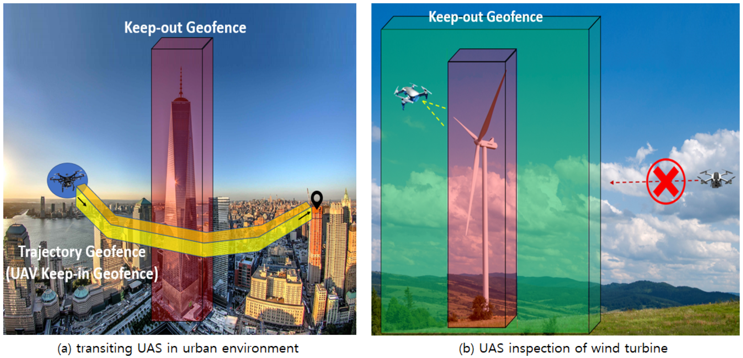
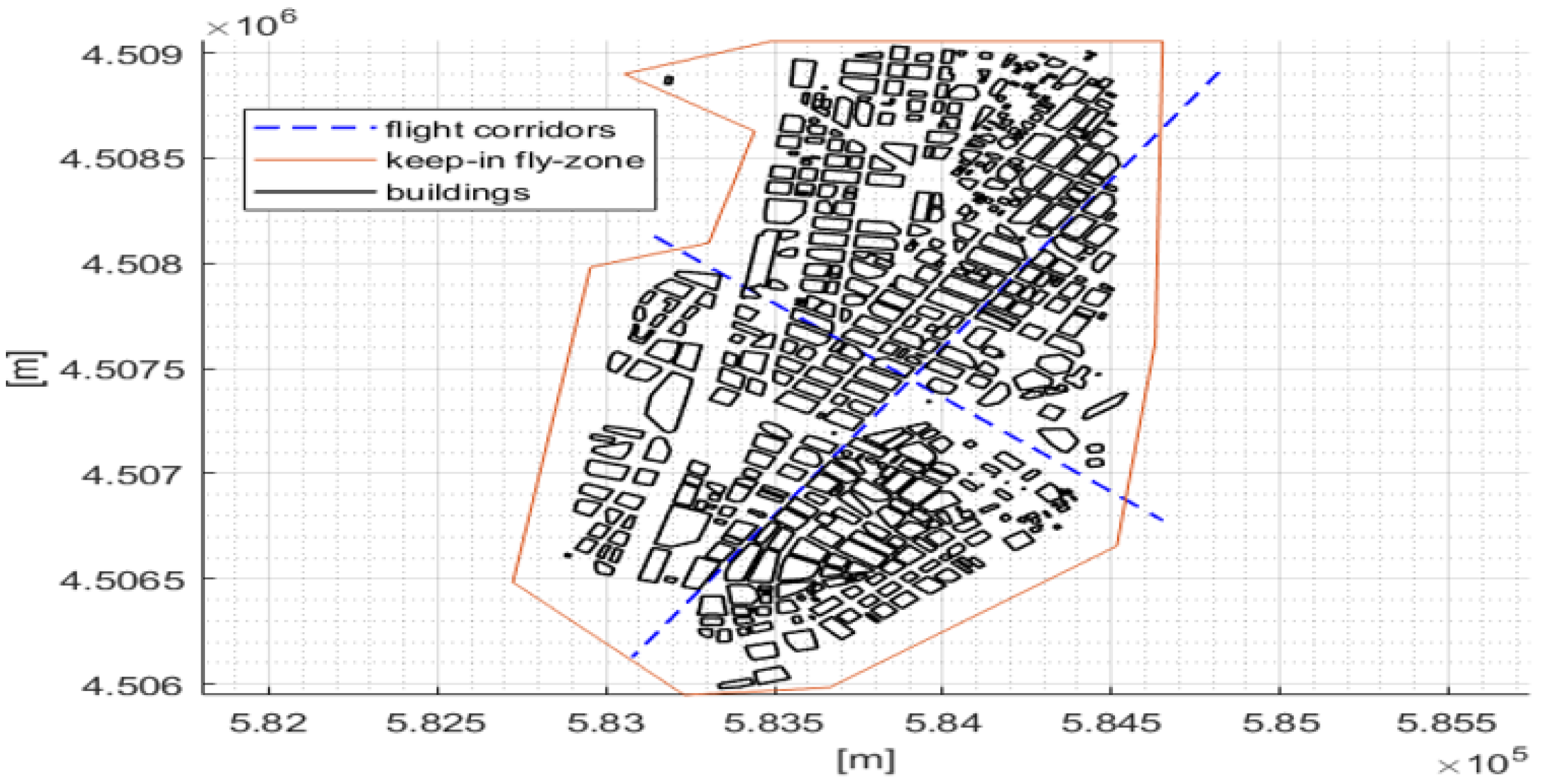
  • The specification of formal algorithms to define keep-in/keep-out geofences for obstacles to plan UAS paths with separation assurance;
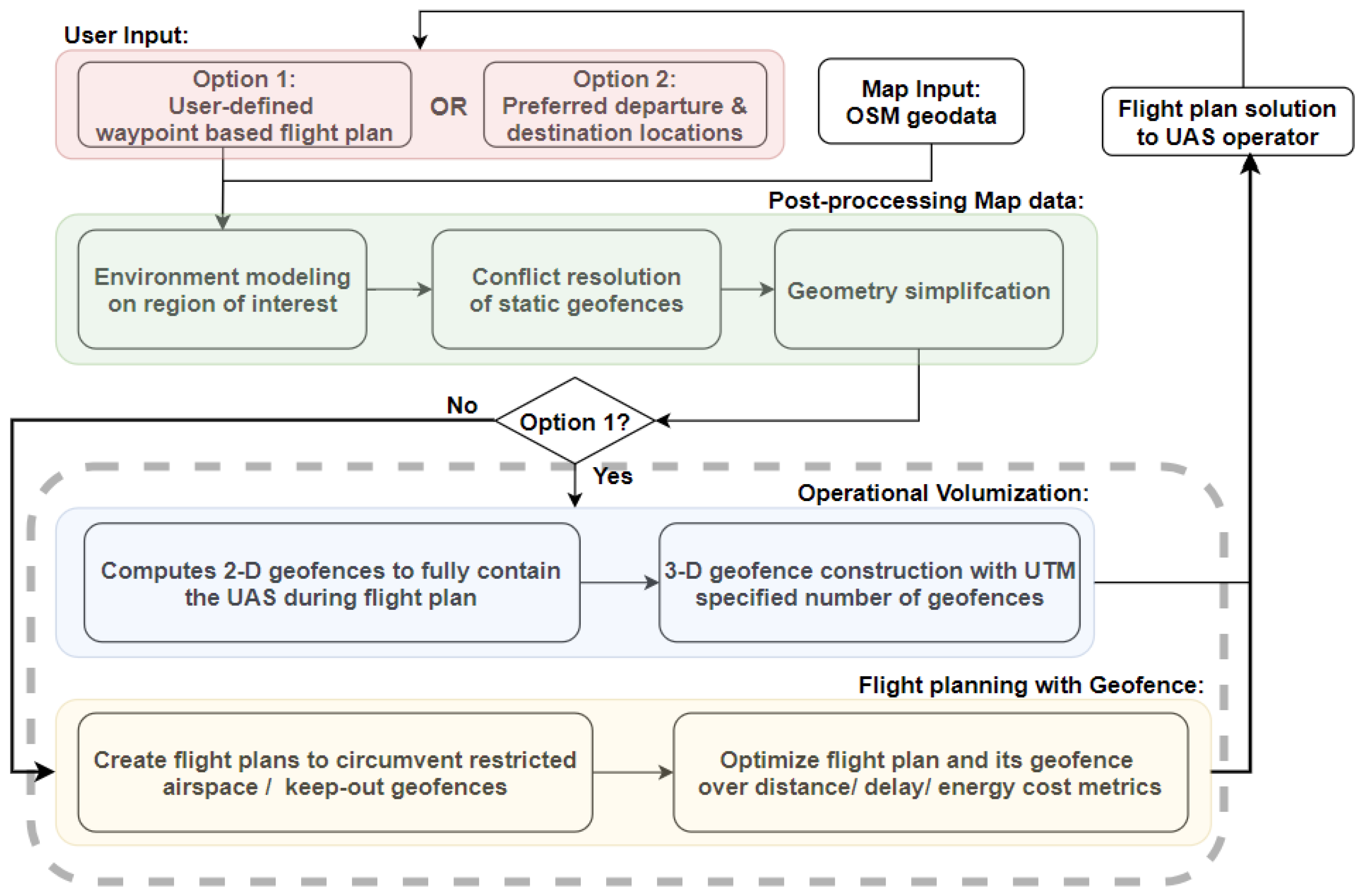
  • The integration of airspace and environmental geofencing processing pipelines with user inputs to construct geofences and geofence-wrapped path plans in a real-world urban environment;
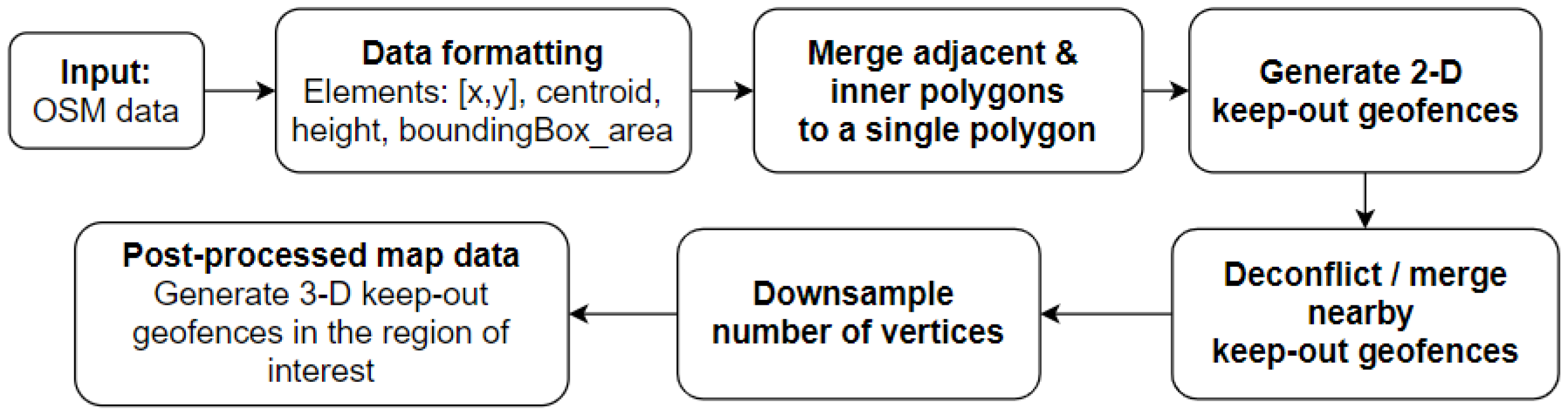
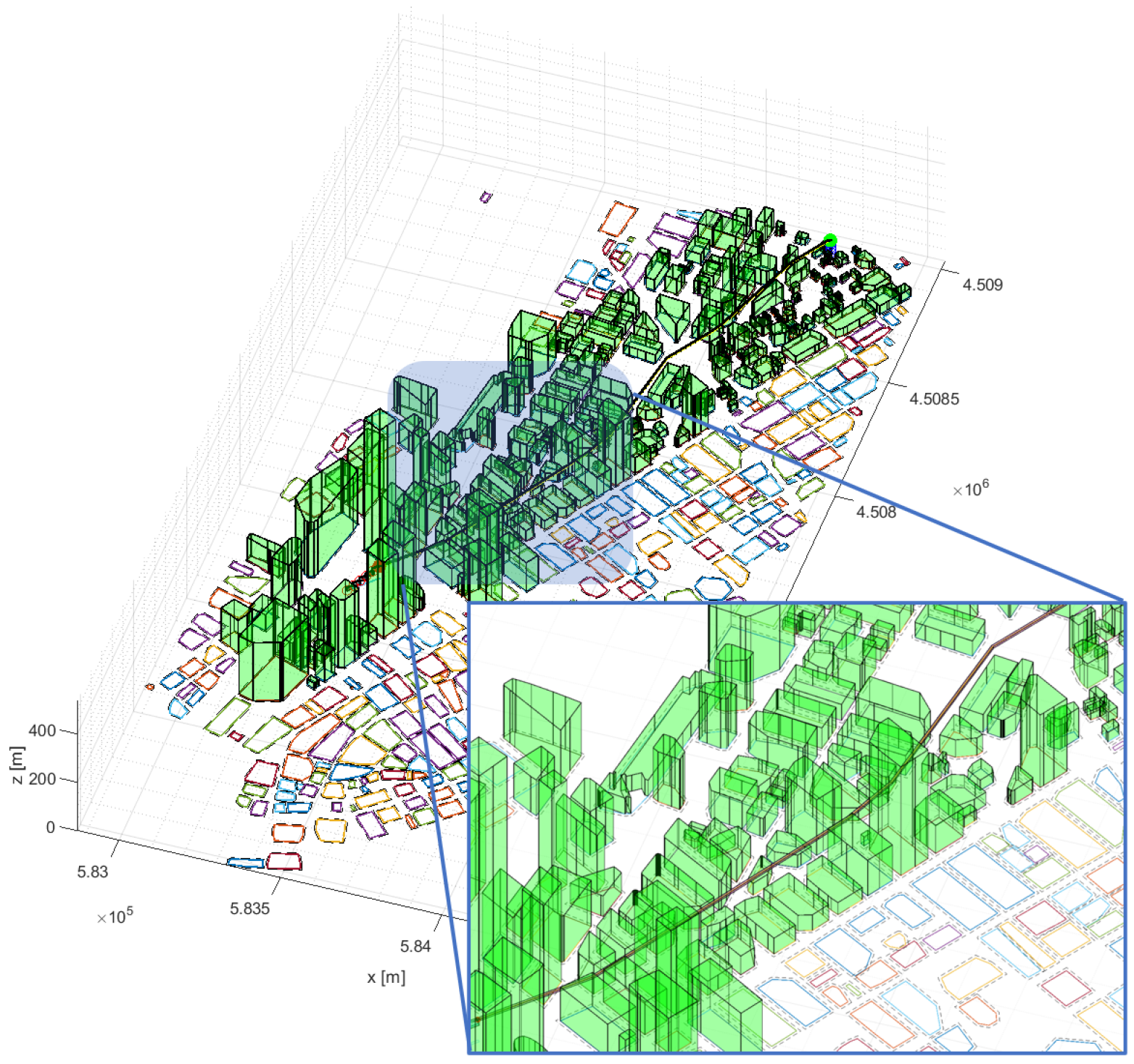
  • Map data processing to generate keep-out geofences around buildings and terrain and a process to simplify a detailed map dataset to support a more compact representation and improved path planning efficiency;
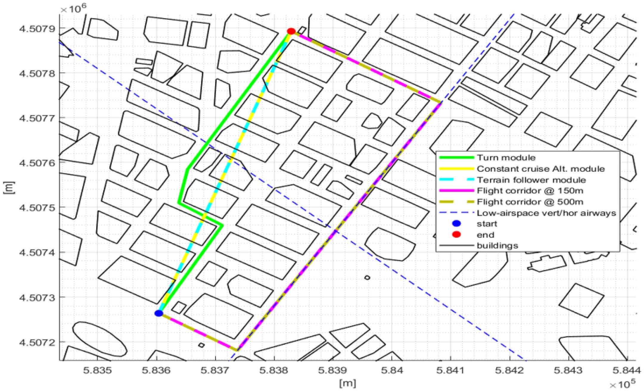
  • A benchmark comparison of our geofenced path planning solutions with a fixed sUAS airway flight corridor design, and a case study of sUAS route deconfliction in shared airspace.
The remaining structure of this paper is organized as follows. Section 2 summarizes previous work in UAS Traffic Management (UTM), sUAS and robotic path planning, and computational geometry methods used in geofencing algorithms. Section 3 defines an airspace geofence, states assumptions made in this work, and introduces sUAS geofencing pipeline algorithms used in the generation of flight trajectory solutions. Section 4 describes OpenStreetMap (OSM) data processing steps to minimize computational time in generating solutions. Section 5 describes Monte Carlo simulation setups that integrate pipeline algorithms with map data processing. Section 6 presents statistics comparing results from our airspace volumization algorithm with a fixed airway flight corridor solution for a region of Manhattan in New York City. Section 7 describes a case study for sUAS route deconfliction, while Section 8 concludes the paper.

2. Literature Review

This section presents related work in UTM, computational geometry, and path planning, all of which are relevant to our geofencing algorithms.

2.1. Unmanned Traffic Management and Geofencing

UTM has been identified as a critical capability for future small UAS operations due to their unique operating profiles at low altitude, near complex infrastructure, and likely in mixed-use airspace [3]. UTM-like concepts have been investigated by industry, government, and academia across the globe. As an example, Single European Sky ATM Research (SESAR) recommended UTM to the European Union (EU) to safely coordinate UAS [15]. Centralized and distributed UTM with airspace volumes distinguished by altitude layer was investigated to deconflict UAS traffic in Sweden [16]. UTM was modeled using a multiplayer network of nodes and airways at low-altitude airspace in Luxembourg [5]. The National Aeronautics and Space Administration (NASA) perhaps first coined the term UTM as a system architecture necessary to accommodate UAS in a low-altitude National Airspace System (NAS) layer not frequently occupied by legacy manned aircraft [3]. Representatives from industry have worked to establish adequate security protocols for managing UTM datalinks [17]. NASA, in cooperation with industry, has pursued a series of flight test events to evaluate cooperative UAS operations in beyond visual line of sight (BVLOS) conditions with a “separation by segregation” geofence design [11]. Airspace capacity estimation was analyzed using keep-in and keep-out geofences in [18]. A roadmap for geofence implementation in urban areas with 5G networks and blockchain was introduced in [19].
Dynamic airspace geofencing algorithms are novel to UTM. Two different but equally important perspectives (i.e., local/global) exist in geofencing designs. One perspective is a classical guidance/navigation/control (GNC) approach, where geofence layering is only generated for the individual UAS that has full knowledge of its control system. This vehicle-centered geofence perspective focuses on controlling UAS to ensure that the vehicle does not violate the geofence boundaries (given expected trajectory tracing errors) [10,20]. In this work, each UAS monitors its real-time state vector relative to geofence boundaries to detect and react to potential breaches given uncertainties due to sensor errors and wind disturbances.
Vehicle-centered geofencing research is important but does not consider properties of the operating area airspace or the ground-based environment. Geofencing has also been researched from an airspace system perspective. With this viewpoint, geofences are managed by UTM to organize airspace structure and improve Situational Awareness (SA). UTM will not model individual UAS capabilities and uncertainties in detail, but it can conservatively monitor UAS travel through an approved geofence to offer impending breach warnings to the UAS and actual boundary violations to all traffic per [21].
SA is a fundamental requirement for all flight operations, autonomous or human-piloted [22,23]; while legacy air Traffic Management (ATM) will remain distinct from UTM in the near term, advanced air mobility (AAM) supporting increasingly to fully autonomous flight will motivate the integration of ATM and UTM over the long term. UTM calls for the automation of airspace management tasks. Airspace organization and protection through geofencing can improve SA and in turn safety. Our algorithms can be integrated into both GNC (onboard) and airspace system (UTM) geofencing realizations.
AAM operations, including but not limited to Urban Air Mobility (UAM), are envisioned to have higher altitudes than 400 AGL, where current UTM is designed to serve. Researchers at NASA and Uber investigated the applicability of UTM to coordinate UAM routes safely and efficiently [24]. In their case studies, “Transit-Based Operational Volumes (TBOVs)” were used to wrap the UAM flight path, a notion analogous to the trajectory keep-in geofence discussed in this paper. Inspired by the static “UAM-authorized airspace” active over a fixed duration [24] as an airspace management alternative to geofencing, in our case studies, we designed fixed flight corridors and simulated sUAS flight missions operating in these flight corridors. This alternative solution offers a benchmark with which our dynamic geofence volumization and path planning solutions are compared (Section 5).

2.2. Computational Geometry

Computational geometry has been used to construct and deconflict airspace geofence volumes and to detect/prevent airspace boundary violations (onboard). A scaling algorithm was developed for two-dimensional keep-in/keep-out concave polygon geofences in [6]. This paper uses vehicle performance constraints and steady wind conditions to generate scaled “warning” and “override” geofence boundaries. Once a UAS crosses one of these boundaries, onboard GNC can trigger a corrective response [25] or flight termination. In [26,27,28], algorithms for polygon set operations (i.e., polygon intersections and unions), polygon clipping, convex hull, and point-in-polygon were developed. We use these algorithms to detect and resolve geofence boundary conflicts and generate new geofence volumes by merging conflicting boundaries. A UAS geofence violation detection method was defined in [7] using Ray Casting [29]. A Triangle Weight Characterization with Adjacency (TWCA) algorithm was developed as a faster real-time geofence violation detection method in [8]. TWCA divides geofence into a finite number of triangles and then finds UAS location in a pre-generated adjacency graph. In [9], a 3-D dynamic geofence (“moving geofence”) was constructed using maximum cruise time, speed, and range of the UAS as a pre-departure flight planning algorithm. This paper also proposes a convex hull approach to find conflicts between current and newly submitted flight plans.

2.3. Path Planning

Determining a collision-free geofence-based flight trajectory is central to the design of our geofencing volumization work. A variety of path planning algorithms were considered. Grid-based path planning methods overlay a fixed-resolution grid on top of the configuration space and find discretized line segment paths connecting start state to destination. This search is fast in low-dimensional space but quickly becomes computationally intractable with high-resolution maps and appreciable travel distance. The most notable grid-based path planning algorithms are A [30] and D [31]. A family of roadmap-based path planning algorithms have been developed to offer a more compact search space optimizing a specific cost metric. For example, a visibility graph [32] minimizes travel distance, while a Voronoi diagram maximizes obstacle clearance distance [33]. The application of cell decomposition [34] offers a compact map for discrete search path planning in an obstacle field. Other path planning methods include potential-field algorithms [35] that efficiently build plans with gradient descents but are subject to local minima issues. Sampling-based path planning algorithms [36] have also been developed and are particularly well suited to planning in uncertain environments. Our work utilizes a visibility graph approach to path planning. This approach allows us to directly translate geofence volumes generated with computational geometry into visibility graph roadmaps. As is discussed below, we scale keep-out geofences to assure safe separation is maintained. Note that a visibility graph does not require a rasterized map, enabling geofences to be represented without distortion or approximation.

3. Definitions and Algorithms

The term airspace geofence was formally defined in [37] to support a common framework for airspace volume reservation in UTM. Our work follows this definition:
Definition 1.
A Geofence g = { n , v [ ] , z f , z c , m , h [ ] } is a volume defined by a list of n vertices in the horizontal plane v = [ ( x 1 , y 1 ) , ( x 2 , y 2 ) , , ( x n , y n ) ] , where n 3 , and an altitude floor z f and ceiling z c . The volume is defined relative to a set of home locations, h i = ( x i , y i , z i , t i ) , where h [ ] is a list of length m 2 . Lateral home positions can be represented as latitude/longitude pairs ( ϕ i , λ i ) or locally referenced Cartesian coordinates ( x i , y i ) . z i is the altitude of the home location above Mean Sea Level (MSL). t i is the activation time for home location i where 1 i m . t m is the deactivation time for geofence g. For consistency, Cartesian coordinates and altitudes are defined in meters and activation/deactivation times are in seconds.
This data structure supports geofence types: static, durational, and dynamic. A static geofence has a permanent fixed home location h [ ] and typically surrounds physical obstacles such as buildings or sensitive areas (i.e., no-fly zones). A durational geofence is active over a finite time interval with a fixed home location h [ ] . A dynamic geofence is active over a specific time interval; its home location can move over time.
The following simplifying assumption is made in this paper to facilitate path planning and eliminate the need for traffic deconfliction.
Assumption 1.
One aircraft (e.g., UAS) is allocated to each local geofence volume. No other UAS is permitted to cross into this volume. UTM efficiency therefore relies on minimizing each reserved geofence volume and its duration.
Dynamic airspace volumization for geofencing will enhance safety by wrapping a UAS in an airspace volume that assures separation from other traffic. The below subsections describe our geofencing algorithm pipeline for UTM, where flight plans are designed with keep-in/keep-out geofencing volumes on a low-altitude airspace map. Three-dimensional trajectory keep-in geofence volumes safely wrapping UAS flight paths are described in Section 3.1, keep-out geofence construction for a low-altitude urban map is described in Section 3.2, and geofence-based path planning solutions are illustrated in Section 3.3.

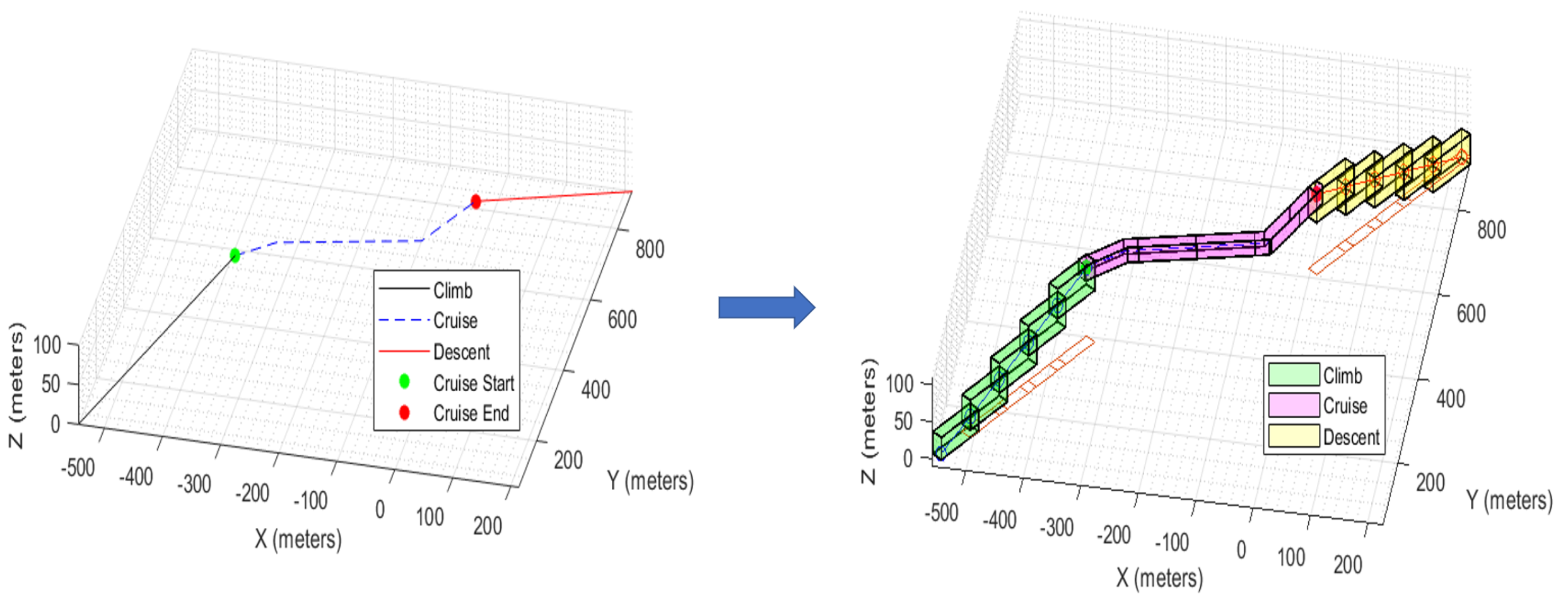
3.1. Airspace Operational Volumization

Operational volumization constructs a trajectory keep-in geofence overlaid on a user-defined 3-D flight trajectory. Climb and descent segments are first generated with vehicle dynamics inputs such as velocity and desired time to climb/descend. Then, three-dimensional cruise operational volumes are created between the climb and descent geofence pair. This assures a geofence volume always encloses the flight trajectory with the prescribed safety buffer δ v e h i c l e . This algorithm integrates 2-D flight trajectory operational volumization with the Multiple Staircase Geofence (MSG) algorithm per [13]. Three-dimensional trajectory volumization is shown in Algorithm 1. Figure 3 shows an example of a 3-D trajectory with its corresponding three-dimensional geofence volume. A sequence of geofence volumes is constructed by connecting climb, cruise, and descent geofences with user-specified safety buffers.
Algorithm 1 3D Flight Trajectory Operational Volumization (3dOperVol).
Inputs: 2-D Trajectory waypoints W , Velocity V , Time to Climb t c l i m b , Time to Descent t d e s c , Number of Geofence N g e o , UAS Safety Buffer δ v e h i c l e , Cruise Altitude h c r u i s e
Outputs: 3-D Flight Trajectory P t r a j , 3-D Geofence for 3-D Flight Trajectory G
Algorithm:
1:
[ P c l i m b , G c l i m b ] M S G ( W [ 1 : 2 ] , V , t c l i m b , N g e o , δ v e h i c l e ) ⊲ generate climb geofence
2:
[ P d e s c , G d e s c ] M S G ( W [ e n d 1 : e n d ] , V , t d e s c , N g e o , δ v e h i c l e ) descent geofence
3:
4:
P c r u i s e [ P c l i m b [ e n d 1 : e n d ] , W [ 3 : e n d 2 ] , P d e s c [ 1 : 2 ] ] ⊲ 3-D Cruise flight
5:
[ G c r u i s e ] M S G ( 2 d O p e r V o l ( P c r u i s e , δ v e h i c l e ) , h c r u i s e ) ⊲ Generate cruise geofence
6:
P t r a j [ P c l i m b ; P c r u i s e ; P d e s c ]
7:
G [ G c l i m b ; G c r u i s e ; G d e s c ]
8:
return [ P t r a j , G ]
To minimize airspace volume reservation duration, we utilize the shrinking durational geofence (SDG) and multi-stage durational geofence (MDG) algorithms in [13] for the cruise segment. A shrinking durational geofence (SDG) removes a previously occupied geofence volume at each time update in UTM. A multi-stage durational geofence (MDG) has multiple volumes generated over the flight trajectory with temporal or spatial overlap. For transitions between MDG regions, either temporal or spatial overlap is used to guarantee the UAS is always enclosed by at least one MDG. Overlap offers a buffer in case the UAS flies faster or slower than expected. Note that climb and descent segments utilize multiple staircase geofences so that previously occupied staircase geofences can be removed sequentially.

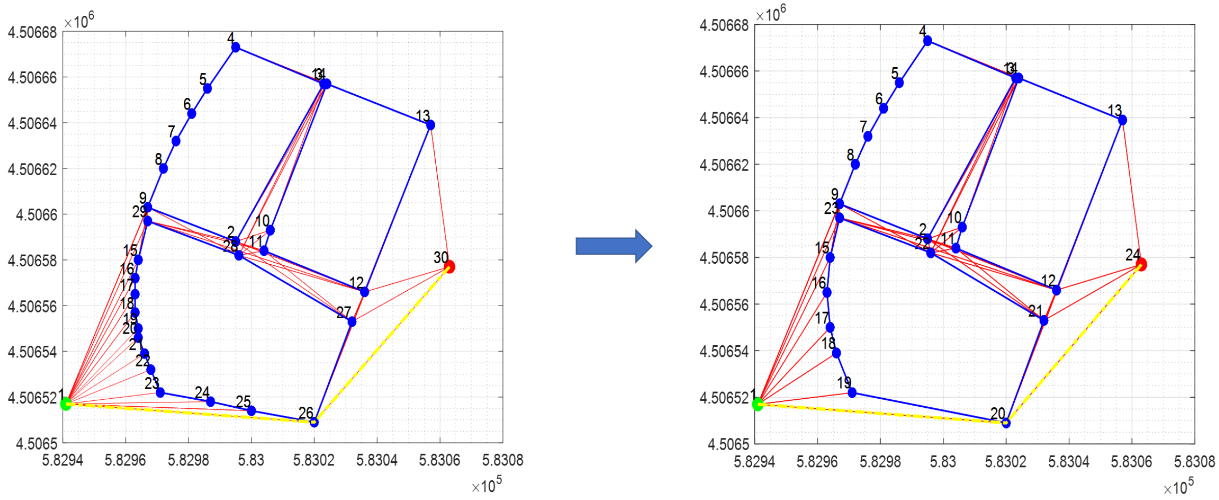
3.2. Constructing a Geofence Volume from an Urban Map

Keep-out geofences are constructed around obstacles (i.e., buildings) to assure separation between UAS and obstacles or no-fly airspace zones. The construction of keep-out geofence volumes from a building and terrain map must be efficiently carried out to constrain the computation time needed to generate geofence-based path planning solutions. For this work, we utilize a visibility graph approach to path planning, as illustrated in Section 3.3. The time complexity of visibility graph generation is O ( n 2 l o g ( n ) ) , where n is the total number of vertices in all polygons. In a real-world environment, the number of keep-out geofences in the urban environment can be significant (i.e., 14,000 building cluster geofence polygons in the southern Manhattan map). We utilize two algorithms to achieve map simplification. First, we downsample geofence vertices in the map as shown in Algorithm 2 per [38] with user-defined parameters n m a x V e r t and p d w n S m p l e . This updated set of keep-out geofences is then used to construct a region of interest (ROI) visibility graph. The ROI in the map is first constructed as a rectangular box surrounding departure and destination points. Then, polygon intersection, point-in-polygon, and convex hull operations are used to define the actual region of interest for which geofence-based path planning solutions are generated. Generation of the flight planning visibility graph ROI is shown in Algorithm 3. Figure 4 shows an example of polygon vertex set downsampling. Figure 5 illustrates an initial rectangular ROI P r e c R O I example.
Algorithm 2 Reduce Map Geofence Vertex Set.
Inputs: Set of Keep-out Geofences S g e o , Downsample Threshold n m a x V e r t , Downsample Tolerance In Percentage p d w n S m p l e
Outputs: Set of Downsampled Keep-out Geofences S d s
Algorithm:
1:
S d s [ ] initialize the output set
2:
3:
for S S g e o do
4:
if  l e n ( S ) / 2 > n m a x V e r t  then
5:
   S o u t D e c i m a t e P o l y ( S , p d w n S m p l e ) downsample polygon vertices
6:
   k 1
7:
  for  j = 1 : l e n ( S o u t )  do
8:
    G [ k : k + 1 ] S o u t [ j , 1 : 2 ] obtain geofence data structure
9:
    k = k + 2
10:
  end for
11:
end if
12:
S d s S d s . a d d ( G )
13:
end for
14:
return S d s
Algorithm 3 Compute Visibility Graph ROI.
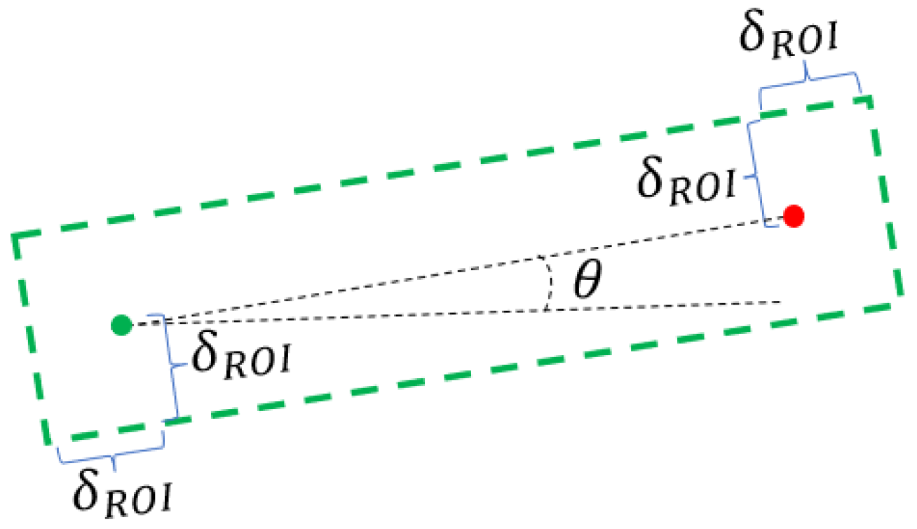
Inputs: Departure Point P s t a r t , Destination Point P e n d , ROI Inital Buffer δ R O I , Keep-out Geofence Set S g e o
Outputs: Keep-out Geofences in ROI S R O I
Algorithm:
1:
P r e c R O I g e t R e c R O I ( P s t a r t , P e n d , δ R O I ) get Rectangular ROI vertices
2:
3:
//get convexhull ROI where geofencing solutions are generated
4:
S i n t e r s e c t [ ] initialize the intersecting geofence set
5:
for S S g e o do
6:
if  s e a r c h I n t e r s e c t ( S , P r e c R O I )  then
7:
   S i n t e r s e c t S i n t s c t . a d d ( S ) Append intersecting geofence
8:
end if
9:
end for
10:
11:
//Search keep-out geofences inside the convex hull P R O I
12:
S R O I [ ] initialize S R O I
13:
P R O I c o n v e x H u l l ( S i n t e r s e c t ) ROI where geofencing solutions are generated
14:
for S S g e o do
15:
if  s e a r c h I n t e r s e c t ( S , P R O I )  then
16:
   S R O I S i n t s c t . a d d ( S ) Append intersecting geofence
17:
end if
18:
end for
19:
return S R O I

3.3. UAS Flight Planning in a Geofenced UTM Airspace

Flight plans are typically optimized over distance, energy usage, and flight time (delay) cost metrics. A UAS configuration space is first obtained from user-defined safety buffers δ v e h i c l e , δ b u i l d i n g around the vehicle and obstacles, respectively. The UAS can then be treated as a point mass in configuration space with obstacle boundaries expanded for safety by:
δ s b = δ v e h i c l e + δ b u i l d i n g .
This safety buffer ensures the vehicle maintains sufficient clearance from any obstacles. δ v e h i c l e and δ b u i l d i n g are user-specified parameters in this work.
Our proposed geofencing pipeline applies three inverse volumization options per [13] based on user-specified departure and destination locations. The first option is a “turn” solution that calculates climb, cruise, and descent flight trajectories that turn away from nearby obstacles, maintaining a minimum-distance path from start to end. For this module, a low-dimensional visibility graph search with Dijkstra’s algorithm [39] plans paths around obstacles (i.e., polygons) defined in a local Cartesian frame. We modeled keep-out geofences on obstacles as open set 3-D polygons extruded from 2-D obstacles with fixed heights. Per Section 2.3, an obstacle-free visibility graph or roadmap space can be constructed from geofence and obstacle polygons without rasterization [32,40].
The second path planning option is a “constant cruise altitude climb” module for which the UAS climbs over no-fly and obstacle volumes until a direct-heading route to the destination is obstacle-free. For this option, a vehicle first climbs to a pre-determined cruise altitude greater than the highest building en route to the destination. Then, the vehicle flies directly to the destination at cruise altitude. As the vehicle approaches the end of its cruise segment, it descends to the destination free of obstacles along the path. The third path planning option is a “vertical terrain follower” module, where a UAS follows the terrain altitude profile en route to the destination, flying as low as possible. This solution minimizes the time a UAS will spend at a high altitude potentially in conflict with other transiting traffic, but it adds complexity to the altitude profile. Figure 6 shows examples of turn, constant cruise altitude, and terrain follower climb solutions per [13].
To determine which of three solutions is best, a weighted cost function over time, distance, and energy is defined:
C = α d t r a v e l + β P t r a v e l + γ t w a i t .
where d t r a v e l , P t r a v e l , a n d t w a i t are distance traveled, power consumption, and time delay until durational geofences disappear, respectively. Weighting factors α , β , a n d γ are user-defined. The path planning solution with minimum cost is then suggested to an operator and/or automation. The flight planning process with geofencing is shown in Algorithm 4. In this algorithm, the departure point, destination point, cruise altitude, and keep-out geofence boundary coordinates are input along with cruise velocity and climb/descent times. For the turn solution, a Rotational Plane Sweep (RPS) algorithm is used to find all straight-line segments connecting line-of-sight vertices to form a visibility graph map. Then, Dijkstra’s algorithm finds the minimum distance path from departure to destination point. For constant altitude climb and terrain follower solutions, points of intersection between a straight line solution path and obstacles are found using a polygon-line intersection operator. Then, obstacle height at the intersection points are extracted from keep-out geofence data. Three-dimensional flight trajectory “turn”, “constant cruise altitude”, and “terrain follower” solutions are wrapped with geofences using Algorithm 1. The best solution is the minimum cost module based on Equation (2). Note that geofence segment duration is not explicitly considered in this paper. Instead, it is assumed the flight trajectory keep-in geofence generated using Algorithm 4 remains active from UAS launch to landing.
Algorithm 4 Flight Planning With Geofencing.
Inputs: Departure Point R s t a r t , Destination Point R e n d , Cruise Altitude h c r u i s e , Keep-out Geofence Boundaries S g e o , Aircraft Velocity V , Time to Climb t c l i m b , Time to Descend t d e s c , Number of Geofences N g e o , UAS Safety Buffer δ v e h i c l e
Outputs: Planned Flight Trajectory P t r a j , Trajectory-wrapping 3-D Geofence Volumes G
Algorithm:
1:
//turn solution module
2:
R V G [ R s t a r t ; S g e o ; R e n d ] ⊲ Vertices of Visibility Graph
3:
[ e d g e s , v e r t _ I D ] R P S ( R V G ) ⊲ get visibility graph edges on the map using RPS
4:
[ R t u r n ] d i j k s t r a P a t h ( R s t a r t , R e n d , e d g e s , v e r t _ I D ) ⊲ get min. distance path
5:
[ P t u r n , G t u r n ] 3 d O p e r V o l ( R t u r n , V , [ t c l i m b , t d e s c ] , N g e o , δ v e h i c l e , h c r u i s e )
6:
D t u r n g e t D i s t ( P t u r n ) ⊲ get turn module flight distance
7:
8:
//climb solution modules
9:
R i n t e r s e c t s e a r c h I n t e r s e c t ( R V G ) ⊲ get intersections from [ R s t a r t ; R e n d ] to S g e o
10:
if R i n t e r s e c t then
11:
    h i n t e r s e c t e x t r a c t H e i g h t ( R i n t e r s e c t , S g e o ) ⊲ get heights at intersections
12:
    h m a x m a x ( h i n t e r s e c t )
13:
   
14:
   //constant cruise altitude
15:
    [ P c o n s t , G c o n s t ] 3 d O p e r V o l ( R i n t e r s e c t , V , [ t c l i m b , t d e s c ] , N g e o , δ v e h i c l e , h m a x )
16:
    D c o n s t g e t D i s t ( P c o n s t ) ⊲ get constant altitude cruise flight distance
17:
   
18:
   //terrain follower
19:
    [ P t e r r , G t e r r ] 3 d O p e r V o l ( R i n t e r s e c t , V , [ t c l i m b , t d e s c ] , N g e o , δ v e h i c l e , h i n t e r s e c t )
20:
    D t e r r a i n g e t D i s t ( P t e r r ) ⊲ get terrain follower flight distance
21:
end if
22:
23:
//cost comparison
24:
[ C m i n , o p t ] c o s t C o m p a r e ( D t u r n , D c o n s t , D t e r r a i n )
25:
if opt == 1 then
26:
    [ P t r a j , G t r a j ] [ p t u r n , G t u r n ] ⊲ best sol: turn module
27:
else if opt == 2 then
28:
    [ P t r a j , G t r a j ] [ p c o n s t , G c o n s t ] ⊲ best sol: constant cruise altitude module
29:
else
30:
    [ P t r a j , G t r a j ] [ p t e r r , G t e r r ] ⊲ best sol: terrain follower module
31:
end if
32:
return [ P t r a j , G t r a j ]

4. Environment Modeling

Map Data Processing

To evaluate the proposed geofencing capability in a complex low-altitude environment, we processed OpenStreetMap (OSM) data for the Manhattan Borough of New York City (USA). OSM is a collaborative global mapping project that creates geographical data and information [41]. OSM is frequently updated and provides map entities including airways, roads, buildings, and more. To minimize map processing overhead for this work, we used pre-processed georeferenced OSM Manhattan building data as described in Ref. [42]. This raw data contain building coordinates represented as polygon vertices, building heights, and street level in WGS 84/UTM zone 18N [43], where units are in meters with East, North, Up (ENU) axes. We applied a combination of set and convex hull [32] operations to simplify geofence geometry for flight planning. Figure 7 shows the flowchart for map data post-processing. After post-processing, the dataset was partitioned into four categories: buildings with heights greater than 20 m, 60 m, 122 m, and 400 m. Depending on sUAS start and end altitude (i.e., roof of building, ground), flight planning utilizes one of these four datasets to generate plans and associated geofence volumes.
Figure 8 shows a map of southern Manhattan with closely spaced building clusters each enclosed by a single keep-out geofence to simplify the Manhattan urban canyon map. Figure 9 shows an example of post-processed georeferenced data and its 3-D keep-out geofence.
A southern Manhattan, New York City map was defined by 14,000 building cluster geofence polygons using the above procedure. To further simplify the map, we downsampled geofence vertices and construct an updated set of keep-out geofences from the ROI visibility graph per Algorithms 2 and 3 in Section 3.2. Figure 10 shows an example of the rectangular ROI, ROI obstacle polygon, and visibility graph generation pipeline. The “turn” flight planning visibility graph was constructed from keep-out geofences inside the ROI along with departure and destination locations.

5. Simulation Setup

Monte Carlo simulations were used to evaluate proposed airspace volumization strategies on the Manhattan map. Figure 11 shows the flowchart of pathfinding logic in our simulation setup. Pathfinding logic comprises four solution modules for the airspace geofencing algorithm. Once the start and end locations were defined, the keep-out geofence ROI polygons (Figure 10) were extracted from post-processed map data. Constant cruise altitude and terrain follower modules were generated by searching the intersection points between the buildings’ keep-out geofences and the line that connects UAS start and end waypoints. A pure turn solution was generated if both start and end locations were on the ground. If either start or end location was on the roof of the building (i.e., inside of the keep-out geofence), a constant cruise altitude algorithm was first used to find the flight path from the start/end point to the outside of the keep-out geofence, and the turn module solution was used to calculate the remaining flight path, creating a combined solution.
Control parameters are shown in Table 1. To offer an experimentally grounded dataset, a prototype quadplane’s power consumption model [44] was used per Table 2 to compute P t r a v e l in climb, cruise, and descent segments. A quadplane is a hybrid quadrotor/fixed-wing UAS designed to vertically takeoff and land in an urban environment. For our simulations, the quadrotor motors were active in all phases of flight; cruise power would otherwise be lower. Cost function weighting factors α = 0.6 , β = 0.2 , γ = 0.0 were chosen to prioritize minimum-distance solutions. Note that γ was set to zero because building obstacles have static or permanent geofences.

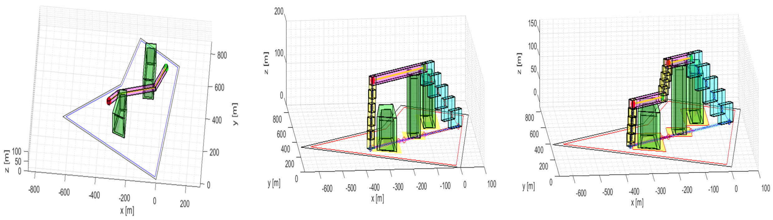
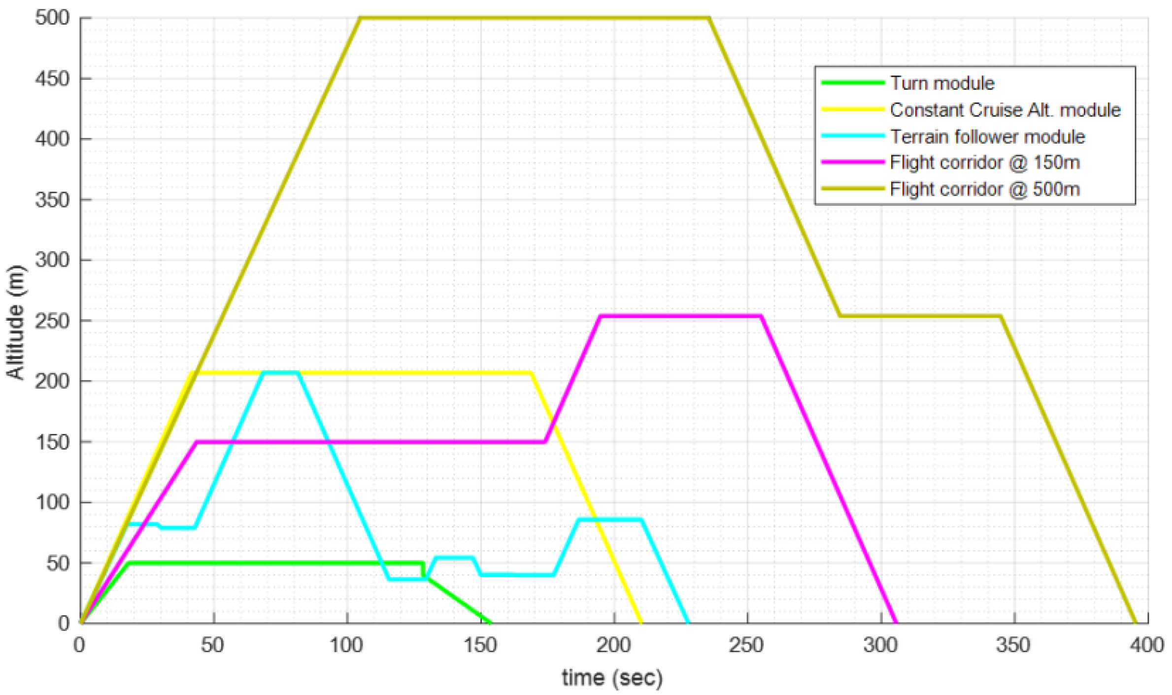
6. Simulation Results

A total of 1010 Monte Carlo simulations were run with our Manhattan maps. For each case, start and destination points were randomly defined. Selected start/end altitudes ranged from 20 m above ground level to the highest building roof. The 20 m value represents an above-ground vertical climb to hover waypoint to ensure the multicopter is well clear of people on the ground when it begins executing its lateral flight plan. If both start and end points had altitudes less than 50 m, the cruise altitude for the turn solution was set at 50 m. Otherwise, cruise altitude was adjusted based on the following condition:
z c r u i s e = m a x { h s t a r t , h e n d } i f h s t a r t > 50 m | | h e n d > 50 m .
Our airspace volumization algorithm used this condition to choose one of the fixed-altitude datasets described in Section 4. As z c r u i s e becomes larger, fewer obstacles were present, so fewer calculations were needed to generate and plan a flight through the visibility graph. For each case, cost values of the four planning options (“turn”, “constant cruise alt.”, “terrain follower”, “combined (constant cruise altitude + turn)” ) were calculated using Equation (2), and the minimum cost solution was selected as the best solution. Note in the Manhattan data the “wait” solution was never used because buildings are permanent, resulting in static geofence obstacles only.
Monte Carlo results offer an opportunity to compare our airspace volumization solutions against a manual fixed airway or “flight corridor” airspace design. A conventional fixed-altitude airway is permanently designated on a map to enable traffic “queues” to organize in a way that can be managed by human air traffic controllers. It is unclear whether UTM will benefit from this legacy design practice, motivating our comparison of path costs for our airspace volumization and fixed airway solutions. Unlike our airspace volumization, fixed airway/flight corridor maps only require a local search for the closest airway to join. The UAS then follows fixed airway routes until exiting over a short final segment to the end state. We generated a pair of low-altitude horizontal and vertical airways through our Lower Manhattan map to illustrate the airways concept and support our evaluation.
The designed vertical airway in Lower Manhattan follows Broadway, the north–south main thoroughfare, from its origin at Bowling Green to Houston Street. The horizontal airway follows Chambers Street from River Terrance in the west to Municipal Plaza in the east, and then follows the Brooklyn Bridge until it reaches the East River. We provided two sets of the same cross airways at 150 m and 500 m to offer each UAS an altitude choice since more obstacles are present at 150 m but the climb will be more substantial to 500 m. Figure 12 shows our manually defined airway corridors. To offer a practical comparison, only randomly generated start and end points that do not lie in the same quadrants (i.e., 712 out of 1010 simulation examples) were considered. If randomly-generated start and end points were located in the same quadrant, the airways were unused, thus offering no benefit to efficiency or airspace organization.
Figure 13 shows a top-down route view comparing our airspace volumization and flight corridor solutions. Cost weights α = 0.6 , β = 0.2 , γ = 0.0 were again used, so d t r a v e l was prioritized in minimizing overall cost. For the illustrated case, the “turn” solution is best. Flight corridor solution cost was in fact typically higher than any of our airspace volumization solutions. For the same example, altitude vs. time plots for each solution are shown in Figure 14. Examples of geofencing solutions are shown in Figure 15, Figure 16 and Figure 17, where three alternative trajectory solutions are generated, ensuring the avoidance of no-fly zones. Building keep-out geofences are shown in green.
For each Monte Carlo simulation, the minimum-cost C solution was compared to flight corridor solution costs at 150 m and 500 m per Table 3. Since the flight corridor at 150 m was almost always better than the flight corridor at 500 m, benchmark data compare the best solution obtained using dynamic airspace volumization with the flight corridor at 150 m. The results indicate our airspace geofencing volumization solutions generally have lower cost than flight corridors at 150 m or 500 m do.
The average distance and power consumption of the two-dimensional straight-line path between each start and destination location are shown in Table 4.
The mean and standard deviation for d t r a v e l , p t r a v e l for the minimum cost airspace volumization solution are summarized in Table 5. The percent frequency distributions of the four solution options are shown in Figure 18.
A similar analysis was performed to compute travel distance and power consumption statistics for the flight corridor solutions at 150 m and 500 m, as shown in Table 6 and Table 7.
Dynamic airspace volumization and flight corridor solutions at 150 m are normalized by the two-dimensional straight-line path parameters, indicating the percent increase in average travel distance and power consumption. A normalized benchmark comparison is shown in Table 8. On average, our 3-D airspace geofencing solution increased travel distance by 15% and power consumption by 3% compared to 2-D straight-line paths from start states to destination states. On the other hand, the travel distance increased by 66 % and power increases by 63% when comparing minimum-cost 3-D geofencing solutions with 150 m flight corridor solutions. This analysis indicates our airspace geofencing algorithm generates routes that offer nontrivial distance (time) and power (energy) reductions relative to flight corridor paths, at least for Manhattan.
All simulations were executed on a standard laptop PC using uncompiled MATLAB code. The mean runtime and standard deviation over all 1010 Monte Carlo simulations were computed. The average runtime was 10.98 s with σ = 12.68 . The minimum runtime was 0.13 s, and the maximum runtime was 90.66 s. As the number of obstacles inside the fly-zone increase, runtime also increased, as might be expected. A more computationally efficient visibility graph algorithm could be implemented in future work [45], particularly with a large obstacle set. Migration from uncompiled MATLAB to a compiled code (e.g., in C++) will also improve performance.
A Monte Carlo simulation generated a suite of random launch (start) and landing (end) points for a single sUAS flying in Lower Manhattan. Start and end points were either located on the ground or a flat building roof to simulate the diverse sUAS flight cases that might be encountered in a densely populated urban environment. Keep-out geofences were generated at each building or around blocks of clustered buildings, representing no-fly zones for the sUAS. Our airspace geofencing pipeline successfully generated flight plans and enclosing geofence volumes for four flight trajectory solution options for all 1010 Monte Carlo simulations. The minimum distance and energy cost was chosen as the best solution. Our geofence-based path planning solutions outperformed a more traditional fixed flight corridor routing option.
Our Monte Carlo simulations did not limit the maximum altitude for UAS flight, so the trajectories for some solutions had cruising altitudes greater than 400 ft AGL, beyond the UTM and sUAS ceiling. Our Monte Carlo results showed the “combined” solution option (i.e., constant cruise and turn) was preferred most often. A maximum altitude constraint would eliminate all solutions that climbed above UTM-managed airspace, likely resulting in the more frequent use of visibility graph “turning” solutions. The results in Table 8 showed that our algorithm generates solutions that are 51% and 60% more efficient than flight corridor solutions at 150 m altitude in terms of normalized average flight distance and power consumption, respectively. It is likely that for AAM airspace corridors accessible to sUAS, above 400 ft AGL will be designated. For longer-distance flights, a flight plan might use an efficient dynamically geofenced route to/from a high-altitude transit tube, potentially requiring a hybrid combination of dynamic flight planning and geofencing at UTM-managed altitudes and fixed corridor transit at altitudes managed by legacy ATM.

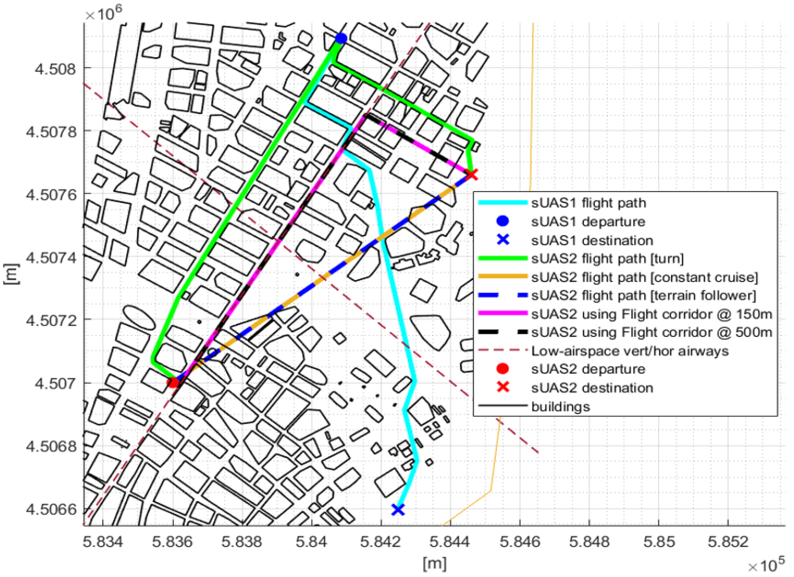
7. Case Study with sUAS Route Deconfliction

The above results describe single geofenced sUAS routes through a complex urban landscape. In general, UTM will manage multiple sUAS in shared airspace. This section presents a case study illustrating how the proposed geofencing pipeline supports multiple-sUAS deconfliction. For this study, we assume airspace is allocated first-come-first-served. Suppose s U A S 1 and s U A S 2 request flight plans each defined by departure and destination coordinates (WGS 84/UTM zone 18N), cruise speed, and targeted cruise altitude as defined in Table 9. Further, suppose s U A S 1 receives approval for its flight plan and associated geofence volume before s U A S 2 contacts UTM. s U A S 2 will then need to plan a flight that avoids the Manhattan terrain and building geofences as well as the flight trajectory geofence wrapping the s U A S 1 route. Figure 19 shows the resulting flight plans for s U A S 2 as a top-down route view comparing our airspace volumization and flight corridor solutions. For this example, altitude vs. time plots for the s U A S 2 solutions are shown in Figure 20.
Since s U A S 1 and s U A S 2 have the same target cruise altitude, a maneuver was required for s U A S 2 to deconflict its “turn” route from the s U A S 1 flight trajectory, making this the longest distance solution option. On the other hand, the “constant cruise altitude” and “terrain follower” solutions were not influenced by the s U A S 1 trajectory because the minimum building height along the straight line path from departure to destination for s U A S 2 was greater than s U A S 1 ’s target cruise altitude. If building height placed s U A S 2 at s U A S 1 ’s cruise altitude, s U A S 2 would also need to climb over the s U A S 1 geofence. Note that if s U A S 1 ’s airspace volume reservation duration was minimized using SDG or MDG, s U A S 2 ’s path had a lower probability of being impacted. Example 3-D s U A S 2 in “turn”, “constant cruise altitude”, “terrain follower” solutions are shown in Figure 21, Figure 22 and Figure 23.

8. Conclusions and Future Work

This paper applied airspace geofencing volumization and path planning to support UTM management of low-altitude airspace. Layered durational geofences wrapping flight trajectories ensure the UAS will fly without conflict in designated or reserved airspace volumes. Our airspace volumization algorithms generated four conflict-free paths for any keep-in/keep-out geofence volume set based on turn, constant cruise, terrain follower and combination turn/cruise options. The algorithm ranked these paths using a weighted distance, energy, and time cost function, then selected the minimum-cost solution. A city map data of Lower Manhattan was used to construct keep-out geofences around buildings. Monte Carlo simulation studies validate our geofence algorithms and support the statistical characterization of performance including run time. A benchmark comparison of our dynamically geofenced flight plans and conventional flight corridor solutions is provided, showing that our solutions reduce flight distance and power compared to fixed corridor solutions. A case study of two sUAS flight planning demonstrated how the proposed geofencing pipeline supports multiple sUAS deconfliction. Algorithms and definitions from this paper can contribute to future UTM dynamic airspace geofencing operational standards.
This work simplifies flight planning to geometric paths. Future work will incorporate aircraft dynamics into flight plans and geofence layer sizing, extend airspace volumization to enclose cooperative groups of sUAS. Additionally, the altitude constraint and other factors such as day/night local population density, GPS dependency, air traffic volume, and vehicle-specific parameters should be incorporated in the geofenced path planning algorithm to generate solutions that are more realistic for UTM-specific applications. We hope to apply machine learning to large-scale flight track data and urban maps to generalize and optimize geofencing volume designs based on area topology, day/night occupancy, infrastructure, and existing air traffic patterns. We will also explore auto-code generation and Python/C++ implementations to improve path planning computational performance.

Author Contributions

Conceptualization, J.K. and E.A.; methodology, J.K. and E.A.; software, J.K.; validation, J.K. and E.A.; writing—original draft preparation, J.K.; writing—review and editing, J.K. and E.A.; visualization, J.K.; supervision, E.A. All authors have read and agreed to the published version of the manuscript.

Funding

This research was funded in part by the Collins Aerospace (Funder grant number: AWD014974) and by NASA (Funder grant number: T18-601046- UMICH).

Institutional Review Board Statement

Not applicable.

Informed Consent Statement

Not applicable.

Data Availability Statement

Not applicable.

Acknowledgments

The authors gratefully acknowledge the following people who supported this research: Mia Stevens for geofencing simulation software and support. Nicholas Liberko for the conceptualization of operational and inverse volumization, Akshay Mathur for the conceptualization of the trajectory geofence and flight power consumption data, and Cosme Ochoa for pre-processed Manhattan map data and documentation.

Conflicts of Interest

The authors declare no conflict of interest.

Abbreviations

The following abbreviations are used in this manuscript:
AAMAdvanced Air Mobility
AGLAbove Ground Level
ATCAir Traffic Control
ATMAir Traffic Management
BVLOSBeyond Visual Line of Sight
d t r a v e l Vehicle travel distance
ERGExplicit Reference Governor
GNCGuidance Navigation and Control
IoTInternet of Things
MDGMulti-staged Durational Geofence
MSGMultiple Staircase Geofence
NASNational Airspace System
n m a x V e r t Allowable maximum number of vertices in a geofence
OSMOpenStreetMap
p d w n S m p l e Downsampling percentage of the number of vertices in a geofence
P t r a v e l Power consumption over d t r a v e l
ROIRegion of Interest
RPSRotational Plane Sweep
SASituational Awareness
SBGSingle Big Geofence
SDGShrinking Durational Geofence
sUASsmall Unmanned Aerial System
TBOVTransit Based Operational Volumnes
TWCATriangle Weight Characterization with Adjacency
t w a i t Wait time until a geofence disappears
UASUnmanned Aircraft System
UTMUAS Traffic Management
UAMUrban Air Mobility
V U A S UAS flight speed
δ b u i l d i n g Safety buffer around a building
δ s b Total safety buffer
δ R O I Safety buffer of initial ROI
δ v e h i c l e Safety buffer of vehicle

References

  1. Joshi, D. Drone Technology Uses and Applications for Commercial, Industrial and Military Drones in 2020 and the Future. December 2019. Available online: https://www.businessinsider.in/tech/news/drone-technology-uses-and-applications-for-commercial-industrial-and-military-drones-in-2020-and-the-future/articleshow/72874958.cms (accessed on 3 January 2021).
  2. Doole, M.; Ellerbroek, J.; Hoekstra, J. Estimation of traffic density from drone-based delivery in very low level urban airspace. J. Air Transp. Manag. 2020, 88, 101862. [Google Scholar] [CrossRef]
  3. Kopardekar, P.; Rios, J.; Prevot, T.; Johnson, M.; Jung, J.; Robinson, J.E. Unmanned aircraft system traffic management (UTM) concept of operations. In Proceedings of the 16th AIAA Aviation Technology, Integration, and Operations Conference, Washington, DC, USA, 13–17 June 2016; pp. 1–16. [Google Scholar]
  4. Barrado, C.; Boyero, M.; Brucculeri, L.; Ferrara, G.; Hately, A.; Hullah, P.; Martin-Marrero, D.; Pastor, E.; Rushton, A.P.; Volkert, A. U-Space Concept of Operations: A Key Enabler for Opening Airspace to Emerging Low-Altitude Operations. Aerospace 2020, 7, 24. [Google Scholar] [CrossRef] [Green Version]
  5. Samir Labib, N.; Danoy, G.; Musial, J.; Brust, M.R.; Bouvry, P. Internet of unmanned aerial vehicles—A multilayer low-altitude airspace model for distributed UAV traffic management. Sensors 2019, 19, 4779. [Google Scholar] [CrossRef] [PubMed] [Green Version]
  6. Stevens, M.N.; Atkins, E.M. Generating Airspace Geofence Boundary Layers in Wind. J. Aerosp. Inf. Syst. 2020, 17, 113–124. [Google Scholar] [CrossRef]
  7. Fu, Q.; Liang, X.; Zhang, J.; Qi, D.; Zhang, X. A Geofence Algorithm for Autonomous Flight Unmanned Aircraft System. In Proceedings of the IEEE 2019 International Conference on Communications, Information System and Computer Engineering (CISCE), Haikou, China, 5–7 July 2019; pp. 65–69. [Google Scholar]
  8. Stevens, M.N.; Rastgoftar, H.; Atkins, E.M. Geofence boundary violation detection in 3D using triangle weight characterization with adjacency. J. Intell. Robot. Syst. 2019, 95, 239–250. [Google Scholar] [CrossRef]
  9. Zhu, G.; Wei, P. Low-altitude uas traffic coordination with dynamic geofencing. In Proceedings of the 16th AIAA Aviation Technology, Integration, and Operations Conference, Washington, DC, USA, 13–17 June 2016; p. 3453. [Google Scholar]
  10. Hermand, E.; Nguyen, T.W.; Hosseinzadeh, M.; Garone, E. Constrained control of UAVs in geofencing applications. In Proceedings of the IEEE 2018 26th Mediterranean Conference on Control and Automation (MED), Zadar, Croatia, 19–22 June 2018; pp. 217–222. [Google Scholar]
  11. Johnson, M.; Jung, J.; Rios, J.; Mercer, J.; Homola, J.; Prevot, T.; Mulfinger, D.; Kopardekar, P. Flight test evaluation of an unmanned aircraft system traffic management (UTM) concept for multiple beyond-visual-line-of-sight operations. In Proceedings of the 12th USA/Europe Air Traffic Management Research and Development Seminar (ATM2017), Seattle, WA, USA, 26–30 June 2017. [Google Scholar]
  12. Dill, E.T.; Young, S.D.; Hayhurst, K.J. SAFEGUARD: An assured safety net technology for UAS. In Proceedings of the 2016 IEEE/AIAA 35th Digital Avionics Systems Conference (DASC), Sacramento, CA, USA, 25–29 September 2016; pp. 1–10. [Google Scholar]
  13. Kim, J.T.; Mathur, A.; Liberko, N.; Atkins, E. Volumization and Inverse Volumization for Low-Altitude Airspace Geofencing. In Proceedings of the AIAA AVIATION 2021 FORUM, Virtual, 2–6 August 2021; p. 2383. [Google Scholar]
  14. Prevot, T.; Rios, J.; Kopardekar, P.; Robinson, J.E., III; Johnson, M.; Jung, J. UAS traffic management (UTM) concept of operations to safely enable low altitude flight operations. In Proceedings of the 16th AIAA Aviation Technology, Integration, and Operations Conference, Washington, DC, USA, 13–17 June 2016. [Google Scholar]
  15. Sesar, J. European Drones Outlook Study Unlocking the Value for Europe; SESAR: Brussels, Belgium, 2016. [Google Scholar]
  16. Sedov, L.; Polishchuk, V. Centralized and distributed UTM in layered airspace. In Proceedings of the 8th International Conference on Research in Air Transportation, Barcelona, Spain, 26–29 June 2018. [Google Scholar]
  17. Jiang, T.; Geller, J.; Ni, D.; Collura, J. Unmanned Aircraft System traffic management: Concept of operation and system architecture. Int. J. Transp. Sci. Technol. 2016, 5, 123–135. [Google Scholar] [CrossRef]
  18. Cho, J.; Yoon, Y. How to assess the capacity of urban airspace: A topological approach using keep-in and keep-out geofence. Transp. Res. Part C Emerg. Technol. 2018, 92, 137–149. [Google Scholar] [CrossRef]
  19. Dasu, T.; Kanza, Y.; Srivastava, D. Geofences in the sky: Herding drones with blockchains and 5G. In Proceedings of the 26th ACM SIGSPATIAL International Conference on Advances in Geographic Information Systems, Seattle, WA, USA, 6–9 November 2018; pp. 73–76. [Google Scholar]
  20. Yoon, H.; Chou, Y.; Chen, X.; Frew, E.; Sankaranarayanan, S. Predictive runtime monitoring for linear stochastic systems and applications to geofence enforcement for uavs. In International Conference on Runtime Verification; Springer: Cham, Switzerland, 2019; pp. 349–367. [Google Scholar]
  21. Stevens, M.N.; Rastgoftar, H.; Atkins, E.M. Specification and evaluation of geofence boundary violation detection algorithms. In Proceedings of the IEEE 2017 International Conference on Unmanned Aircraft Systems (ICUAS), Miami, FL, USA, 13–16 June 2017; pp. 1588–1596. [Google Scholar]
  22. Endsley, M.R. Design and evaluation for situation awareness enhancement. In Proceedings of the Human Factors Society Annual Meeting, Anaheim, CA, USA, 24–28 October 1988; Sage Publications: Los Angeles, CA, USA, 1988; Volume 32, pp. 97–101. [Google Scholar]
  23. Endsley, M.R.; Rodgers, M.D. Situation awareness information requirements analysis for en route air traffic control. In Proceedings of the Human Factors and Ergonomics Society Annual Meeting; SAGE Publications: Los Angeles, CA, USA, 1994; Volume 38, pp. 71–75. [Google Scholar]
  24. Verma, S.A.; Monheim, S.C.; Moolchandani, K.A.; Pradeep, P.; Cheng, A.W.; Thipphavong, D.P.; Dulchinos, V.L.; Arneson, H.; Lauderdale, T.A.; Bosson, C.S.; et al. Lessons learned: Using UTM paradigm for urban air mobility operations. In Proceedings of the 2020 AIAA/IEEE 39th Digital Avionics Systems Conference (DASC), San Antonio, TX, USA, 11–16 October 2020; pp. 1–10. [Google Scholar]
  25. Stevens, M.N.; Atkins, E.M. Multi-mode guidance for an independent multicopter geofencing system. In Proceedings of the 16th AIAA Aviation Technology, Integration, and Operations Conference, Washington, DC, USA, 13–17 June 2016; p. 3150. [Google Scholar]
  26. Weiler, K. Polygon comparison using a graph representation. In Proceedings of the 7th Annual Conference on Computer Graphics and Interactive Techniques, Seattle, WA, USA, 14–18 July 1980; pp. 10–18. [Google Scholar]
  27. Sklansky, J. Finding the convex hull of a simple polygon. Pattern Recognit. Lett. 1982, 1, 79–83. [Google Scholar] [CrossRef]
  28. Haines, E. Point in Polygon Strategies. Graph. Gems 1994, 4, 24–46. [Google Scholar]
  29. Hormann, K.; Agathos, A. The point in polygon problem for arbitrary polygons. Comput. Geom. 2001, 20, 131–144. [Google Scholar] [CrossRef] [Green Version]
  30. Duchoň, F.; Babinec, A.; Kajan, M.; Beňo, P.; Florek, M.; Fico, T.; Jurišica, L. Path planning with modified a star algorithm for a mobile robot. Procedia Eng. 2014, 96, 59–69. [Google Scholar] [CrossRef] [Green Version]
  31. Stentz, A. Optimal and efficient path planning for partially known environments. In Intelligent Unmanned Ground Vehicles; Springer: Boston, MA, USA, 1997; pp. 203–220. [Google Scholar]
  32. De Berg, M.; Van Kreveld, M.; Overmars, M.; Schwarzkopf, O. Computational geometry. In Computational Geometry; Springer: Berlin/Heidelberg, Germany, 1997; pp. 1–17. [Google Scholar]
  33. Latombe, J.C. Robot Motion Planning; Springer Science & Business Media: New York, NY, USA, 2012; Volume 124. [Google Scholar]
  34. Lingelbach, F. Path planning using probabilistic cell decomposition. In ICRA’04, Proceedings of the IEEE International Conference on Robotics and Automation, New Orleans, LA, USA, 26 April–1 May 2004; IEEE: New York, NY, USA, 2004; Volume 1, pp. 467–472. [Google Scholar]
  35. Hwang, Y.K.; Ahuja, N. A potential field approach to path planning. IEEE Trans. Robot. Autom. 1992, 8, 23–32. [Google Scholar] [CrossRef] [Green Version]
  36. Burns, B.; Brock, O. Sampling-based motion planning using predictive models. In Proceedings of the 2005 IEEE International Conference on Robotics and Automation, Barcelona, Spain, 18–22 April 2005; pp. 3120–3125. [Google Scholar]
  37. Stevens, M.; Atkins, E. Geofence Definition and Deconfliction for UAS Traffic Management. IEEE Trans. Intell. Transp. Syst. 2021, 22, 5880–5889. [Google Scholar] [CrossRef]
  38. Semechko, A. Decimate 2D Contours/Polygons. 2018. Available online: https://github.com/AntonSemechko/DecimatePoly (accessed on 3 January 2021).
  39. Bondy, J.A.; Murty, U.S.R. Graph Theory with Applications; Macmillan: London, UK, 1976; Volume 290. [Google Scholar]
  40. Huang, H.P.; Chung, S.Y. Dynamic visibility graph for path planning. In Proceedings of the 2004 IEEE/RSJ International Conference on Intelligent Robots and Systems (IROS) (IEEE Cat. No. 04CH37566), Sendai, Japan, 28 September–2 October 2004; Volume 3, pp. 2813–2818. [Google Scholar]
  41. Haklay, M.; Weber, P. Openstreetmap: User-generated street maps. IEEE Pervasive Comput. 2008, 7, 12–18. [Google Scholar] [CrossRef] [Green Version]
  42. Ochoa, C.A.; Atkins, E.M. Urban Metric Maps for Small Unmanned Aircraft Systems Motion Planning. arXiv 2021, arXiv:2102.07218. [Google Scholar] [CrossRef]
  43. Kumar, M. World geodetic system 1984: A modern and accurate global reference frame. Mar. Geod. 1988, 12, 117–126. [Google Scholar] [CrossRef]
  44. Mathur, A.; Atkins, E.M. Design, Modeling and Hybrid Control of a QuadPlane. In Proceedings of the AIAA Scitech 2021 Forum, Virtual, 11–22 January 2021; p. 374. [Google Scholar]
  45. Hershberger, J.; Suri, S. An optimal algorithm for Euclidean shortest paths in the plane. SIAM J. Comput. 1999, 28, 2215–2256. [Google Scholar] [CrossRef] [Green Version]
Figure 1. UAS airspace geofencing examples. The left figure shows a keep-out geofence (red) around One World Trade Center in New York City. A transiting UAS keeps clear of this geofence with a path wrapped by a trajectory or keep-in geofence (yellow). The right figure shows a wind turbine being inspected by a small UAS. During inspection, the usual wind turbine keep-out geofence (red) is expanded as depicted in green to also enclose the inspection UAS. Any other nearby UAS will keep clear of this expanded keep-out geofence (green) during inspection activities. This geofence design assures separation between the two illustrated UAS.
Applsci 12 00576 g001
Figure 2. Airspace and environment geofencing functionality and data flow.
Applsci 12 00576 g002
Figure 3. Example application of Algorithm 1. A sample 3-D flight path is shown on the left. A corresponding flight trajectory keep-in geofence is shown on the right.
Applsci 12 00576 g003
Figure 4. Example of reducing number of vertices to simplify the associated visibility graph. The left illustration shows three original polygons. The right illustration shows the polygons after applying the vertex downsampling algorithm. n m a x V e r t and p d w n S m p l e are 15 and 60%, respectively. The time complexity of visibility graph generation is O ( n 2 l o g ( n ) ) , where n is the total number of vertices in all polygons. The number of vertices in the lower polygon illustrated here is reduced from 15 to 9.
Applsci 12 00576 g004
Figure 5. Illustration of rectangular ROI generation. Start point, destination point, and ROI initial buffer size δ R O I are used to initialize the rectangular ROI per Algorithm 3.
Applsci 12 00576 g005
Figure 6. Three candidate flight planning solutions respecting keep-out airspace geofence and obstacle “no-fly” volumes. A turn solution uses a visibility graph to define a constant-altitude path around no-fly zones (left). A cruise altitude solution climbs to an altitude greater than the highest building enroute to the destination (center). The terrain follower defines an altitude profile maintaining minimum safe clearance or greater from no-fly zones (right).
Applsci 12 00576 g006
Figure 7. Flowchart of post-processing map data. OSM data were converted to a MATLAB format, then processed using polygon set convex hull operators to reduce the number of keep-out geofences in the region of interest (ROI), the area between departure and destination points. If the number of vertices in a geofence is greater than threshold n m a x V e r t , it is downsampled to p d w n S m p l e . n m a x V e r t and p d w n S m p l e are user-defined parameters set to 15 and 60%, respectively, in this work. Algorithms 2 and 3 are used in finding ROI and reducing number of map vertices. Three-dimensional keep-out geofences around buildings are generated with safety buffer δ b u i l d i n g .
Applsci 12 00576 g007
Figure 8. Post-processing map data for southern Manhattan. Buildings with heights greater than 20 m are shown. The rightmost plot shows keep-out geofences enclosing building clusters (black solid lines), individual building keep-out geofences (black dashed lines), and building outlines (colored lines). Geofence maps for 60 m, 122 m, and 400 m altitude cross-sections are constructed in the same manner.
Applsci 12 00576 g008
Figure 9. Post-processed georeferenced data for the One World Trade Center building in Manhattan. The top left and right show raw OSM data side and top views, respectively. The bottom left and right show post-processed keep-out geofence data (shaded in green) side and top views, respectively.
Applsci 12 00576 g009
Figure 10. Keep-out geofence polygon extraction for UAS flight planning. The initial ROI (green dashed line) is a rectangular box per Figure 5. Keep-out geofences (solid black lines) inside or intersecting the rectangular ROI box are found using polygon intersection and point-in-polygon operations. The final ROI (red dashed line) is the convex hull around these keep-out geofences. For our simulation, δ R O I = 150 m.
Applsci 12 00576 g010
Figure 11. Flow chart of pathfinding logic for different start and end locations. In the chart, V.G. abbreviates visibility graph, and h b l d g is the height of a geofence around a cluster of buildings. If the departure/destination is not inside the keep-out geofence ROI box, h b l d g at start/end point is set to street/terrain altitude.
Applsci 12 00576 g011
Figure 12. Example horizontal and vertical airway corridors in Manhattan.
Applsci 12 00576 g012
Figure 13. Top-down view of example flight paths for airspace volumization and fixed flight corridor solutions. Distances traveled are 770 m (turn), 1051 m (constant cruise), 1139 m (terrain follower), 1528 (150 m flight corridor), and 1977m (500 m flight corridor).
Applsci 12 00576 g013
Figure 14. Flight altitude time histories for airspace volumization and flight corridor solutions for Figure 13 example.
Applsci 12 00576 g014
Figure 15. Example of a 3-D geofence wrapping a “turn” flight plan solution. Polyhedra in green denote keep-out geofences around buildings near the trajectory’s keep-in geofence. The remaining 2-D polygons denote keep-out geofences around buildings that are more distant from the sUAS flight path.
Applsci 12 00576 g015
Figure 16. Example 3-D geofencing solution for a “constant cruise altitude” flight plan solution. Polyhedra in green denote keep-out geofences around buildings near the trajectory’s keep-in geofence. The remaining 2-D polygons denote keep-out geofences around buildings that are more distant from the sUAS flight path.
Applsci 12 00576 g016
Figure 17. Example 3-D geofencing solution for a “terrain follower” flight plan solution. Polyhedra in green denote keep-out geofences around buildings near the trajectory’s keep-in geofence. The remaining 2-D polygons denote keep-out geofences around buildings that are more distant from the sUAS flight path.
Applsci 12 00576 g017
Figure 18. Percent frequency distribution of minimum-cost solutions over Monte Carlo simulations.
Applsci 12 00576 g018
Figure 19. Top-down view of s U A S 2 sample solutions. Five flight trajectory solutions are generated for s U A S 2 . Each solution provides route deconfliction from Manhattan terrain and building geofences and from the s U A S 1 flight trajectory geofence. Distances traveled are 2008 m (turn), 1585 m (constant cruise), 1634 (terrain follower), 1983 (150 m flight corridor), and 2395 (500 m flight corridor). The minimum-cost solution for s U A S 2 is the constant cruise altitude option.
Applsci 12 00576 g019
Figure 20. Flight altitude time histories for airspace volumization and flight corridor solutions for s U A S 2 in Figure 19 example.
Applsci 12 00576 g020
Figure 21. Example of a 3-D geofence wrapping a “turn” flight plan for s U A S 2 . The s U A S 2 trajectory is shown in black, and the s U A S 1 trajectory is shown in blue. Polyhedra (green) denote keep-out geofences around buildings. The remaining 2-D polygons denote keep-out geofences around buildings that are outside the combined ROI.
Applsci 12 00576 g021
Figure 22. Example of a 3-D geofence wrapping a “constant cruise altitude” flight plan for s U A S 2 . The s U A S 2 trajectory is shown in black, and the s U A S 1 trajectory is shown in blue. Polyhedra (green) denote keep-out geofences around buildings. The remaining 2-D polygons denote keep-out geofences around buildings that are outside the combined ROI.
Applsci 12 00576 g022
Figure 23. Example of a 3-D geofence wrapping a “terrain follower” flight plan for s U A S 2 . The s U A S 2 trajectory is shown in black, and the s U A S 1 trajectory is shown in blue. Polyhedra (green) denote keep-out geofences around buildings. The remaining 2-D polygons denote keep-out geofences around buildings that are outside the combined ROI.
Applsci 12 00576 g023
Table 1. Control parameters for geofenced flight planning case studies.
V vehicle δ vehicle δ building N geofence z cruise
5 (m/s)2 (m)5 (m)550 (m)
Table 2. Flight power consumption data from [44].
ClimbDescentForward Flight
312 (J/s)300 (J/s)328 (J/s)
Table 3. Number of cases where airspace volumization v o l has minimum cost (left) and number of cases where the flight corridor at 150 m has lower cost than the corridor at 500 m.
# { C vol . method < C 150 m } # { C 150 m < C 500 m }
698 out of 712 cases702 out of 712 cases
Table 4. Average distance (d), power consumption (P), and minimum and maximum distances of 2D straight-line paths between start and destination states for the Monte Carlo simulations.
μ d 2 D path μ P 2 D path min { d 2 D path } max { d 2 D path }
1391 (m)91259 (J)189 (m)3003 (m)
Table 5. Mean μ and standard deviation σ of the minimum-cost airspace volumization solution.
μ d travel σ d travel μ P travel σ P travel min { d travel } max { d travel }
1595 (m)606 (m)94,338 (J)39,609 (J)254 (m)3349 (m)
Table 6. Mean μ and standard deviation σ of 150 m flight corridor solutions.
μ d 150 m σ d 150 m μ P 150 m σ P 150 m min { d 150 m } max { d 150 m }
2303 (m)820 (m)149,084 (J)53,449 (J)479 (m)4464 (m)
Table 7. Mean μ and standard deviation σ of 500 m flight corridor solutions.
μ d 500 m σ d 500 m μ P 500 m σ P 500 m min { d 500 m } max { d 500 m }
2796 (m)788 (m)179,363 (J)51,502 (J)1142 (m)4836 (m)
Table 8. Normalized travel distance comparison between airspace geofencing and 150 m flight corridor solutions.
μ d travel / μ d 2 D path μ P travel / μ P 2 D path μ d 150 m / μ d 2 D path μ P 150 m / μ P 2 D path
115 (%)103 (%)166 (%)163 (%)
Table 9. Flight plan parameters for s U A S 1 and s U A S 2 .
P Departure ( m ) P Destination ( m ) V UAS ( m / s ) h targetCruise ( m )
s U A S 1 [584,085; 4,508,093; 0][584,248; 4,506,598; 0]3050
s U A S 2 [583,600; 4,507,000; 0][584,460; 4,507,660; 0]2050
Publisher’s Note: MDPI stays neutral with regard to jurisdictional claims in published maps and institutional affiliations.

