A New Vibration Controller Design Method Using Reinforcement Learning and FIR Filters: A Numerical and Experimental Study

Abstract

High-dimensional high-frequency continuous-vibration control problems often have very complex dynamic behaviors. It is difficult for the conventional control methods to obtain appropriate control laws from such complex systems to suppress the vibration. This paper proposes a new vibration controller by using reinforcement learning (RL) and a finite-impulse-response (FIR) filter. First, a simulator with enough physical fidelity was built for the vibration system. Then, the deep deterministic policy gradient (DDPG) algorithm interacted with the simulator to find a near-optimal control policy to meet the specified goals. Finally, the control policy, represented as a neural network, was run directly on a controller in real-world experiments with high-dimensional and high-frequency dynamics. The simulation results show that the maximum peak values of the power-spectrum-density (PSD) curves at specific frequencies can be reduced by over 63%. The experimental results show that the peak values of the PSD curves at specific frequencies were reduced by more than 47% (maximum over 52%). The numerical and experimental results indicate that the proposed controller can significantly attenuate various vibrations within the range from 50 Hz to 60 Hz.

1. Introduction

Active vibration control is a challenging problem with high-dimensional, high-frequency and complex dynamics. Many conventional vibration controllers have been presented to solve this problem. For instance, PID controllers [1,2,3,4], which are not very suitable for high-dimensional vibration-control problems, and the determination of the controller parameters requires substantial design effort; LQR controllers [5,6,7], which are suitable for the systems that can be formulated by state-space equations; FxLMS controllers [8,9,10], which require the construction of a reference signal and the identification of a secondary path. It was found that, although these conventional controllers are usually effective, they require substantial engineering effort, design effort and expertise.

A new simple method for vibration-controller design is made possible by using RL. The parameters of the controller are automatically obtained by reinforcement-learning algorithms. Moreover, the new method is a data-driven method, which means that it does not require the physical information of the system, such as the mass matrix, stiffness matrix or damping matrix. Therefore, the new method requires less engineering effort and design effort in comparison with the conventional controller design methods.

Actually, RL has been widely used for building agents to learn complex control in complex environments, and it has achieved some successes in a variety of domains [11,12,13,14,15]. Moreover, its applicability has been extended to the vibration-control domain, such as the vibration control of the suspension [16,17,18,19], manipulator [20,21,22], magneto rheological damper [23,24], flexible beam/plate [25,26,27], etc.

In suspension vibration-control problems [16,17,18,19], the controllers are trained to suppress the vibration caused by road profiles, and they are only validated by numerical simulations. Bucak et al. [16] used a stochastic actor–critic reinforcement-learning control algorithm to provide control forces to a nonlinear quarter-car active-suspension model subjected to a sinusoidal road profile. The simulation results showed that the new algorithm stabilized the suspension very quickly. Kim et al. [17] applied the DDPG (deep deterministic policy gradient) algorithm to the vibration-control simulation of a quarter-vehicle active-suspension model. The quarter-vehicle model with a trained agent (controller) was tested at the low-frequency cosine road and step road, which confirmed the effectiveness of the DDPG algorithm. Liu et al. [18] presented an improved DDPG algorithm using empirical samples, and they applied it to a quarter-vehicle semiactive-suspension vibration-control simulation. The simulation results showed that, compared with the passive suspension, the semiactive suspension with the improved DDPG algorithm could better adapt to various road levels and vehicle speeds. Han et al. [19] presented a PPO-based vibration-control strategy for a vehicle semiactive-suspension system, in which the designed reward function realizes the dynamic adjustment according to the road-condition changes. The simulation results showed that the body acceleration was reduced by 46.93% under the continuously changing road. These suspension vibration-control studies mainly considered single-input control problems.

In flexible-manipulator control problems [20,21,22], the controllers are trained to suppress the transient vibration, as well as to follow the given trajectories. Ouyang et al. [20] applied the actor–critic algorithm for a single-link flexible manipulator in an attempt to suppress the vibration due to its flexibility and lightweight structure. In the experiment, when the single link was given a desired position, the reinforcement-learning control could obtain a satisfactory tracking and vibration-suppression performance. He et al. [21] investigated the actor–critic reinforcement-learning control of a flexible two-link manipulator by a numerical and experimental study. In the simulation and experiment, when the links were given desired trajectories, the reinforcement-learning control had feasibility and stability in suppressing the vibration. Long et al. [22] presented a combined-vibration-control method for a hybrid-structured flexible manipulator based on sliding-mode control and reinforcement learning. The experimental results showed that the combined control method had good robustness to the tip trajectory and tip-load mass under the condition that the learning parameters of the controller remained unchanged.

In terms of the vibration-control problems of magneto rheological dampers [23,24], as the controller was designed based on Q-learning [28], they are theoretically not suitable for high-dimensional continuous-action spaces. Park et al. [23] proposed a novel reinforcement-learning method based on Q-learning for the vibration control of a magneto rheological elastomer. The experimental results showed that the proposed method could minimize the vibration level with respect to the tonal disturbance or sine-sweep disturbance. Yuan et al. [24] proposed a semiactive control strategy of a magneto rheological damper based on the Q-learning algorithm, and the simulation results showed that it was better than simple bang-bang control.

In the vibration-control problems of flexible beams or plates [25,26,27], accurate finite element models are constructed as the simulation environment, and then reinforcement-learning algorithms, such as the soft actor–critic algorithm, DDPG algorithm and multiagent twin delayed DDPG algorithm, are applied to train the vibration controllers. Finally, the well-trained controllers are validated in experiments. The simulation and experimental results demonstrate that the controllers trained by the proposed RL algorithms have better control effects compared with PD control. However, an accurate finite element model is difficult to build for complex vibrating systems, and the proper PD parameters are difficult to estimate.

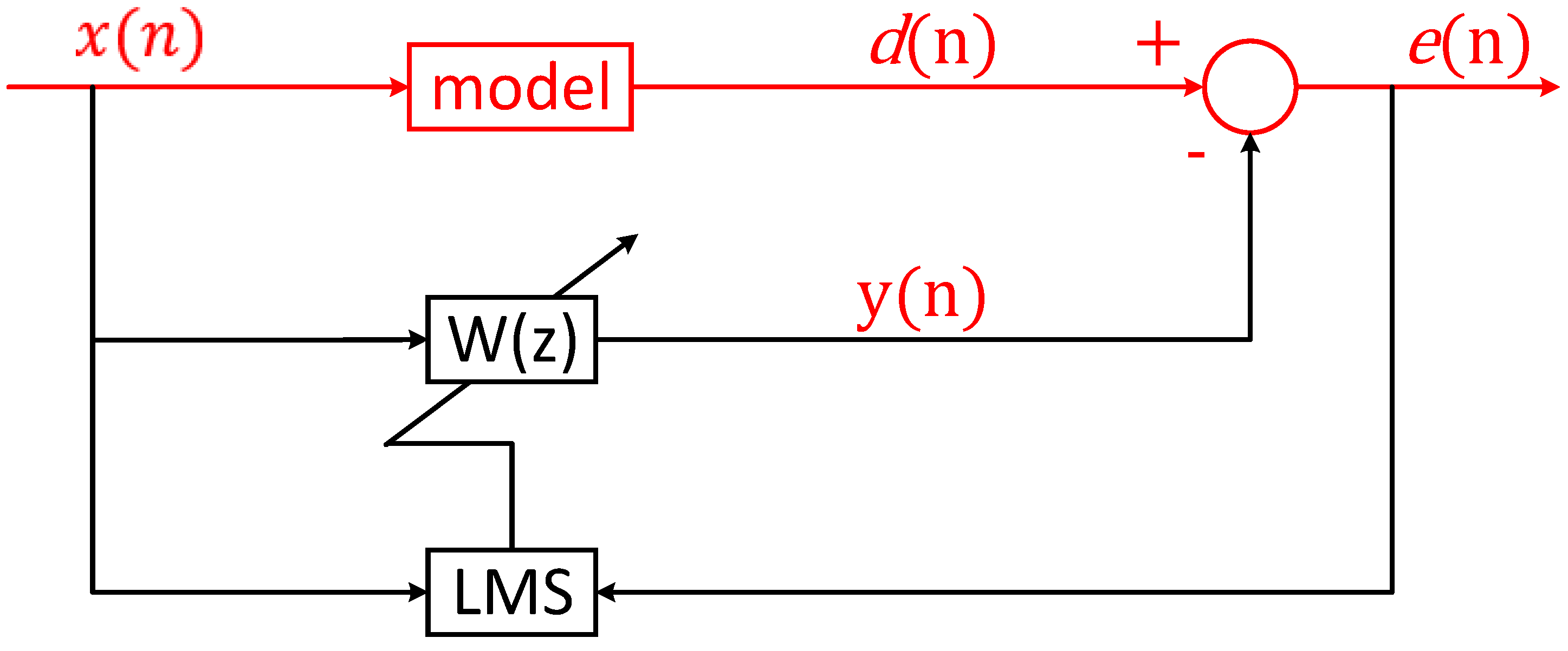
Although RL algorithms were applied in the above vibration-control research, they mainly considered vibration-control problems of low dimension (for instance, the single-input suspension control problem) and simple dynamics, such as link, beam, plate, quarter-car, etc., simulation models. However, this paper solved the multi-input/multi-output real-world vibration-control problem within a frequency range by using RL and an FIR filter, which was inspired by the least-mean-square (LMS) adaptive algorithm. To the best of the authors’ knowledge, this is the first time that the high-dimensional high-frequency vibration-control problem has been solved by using reinforcement learning.

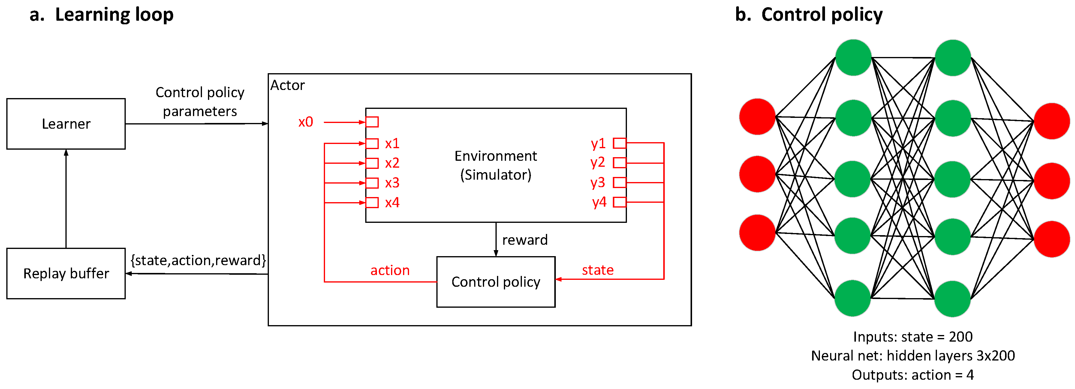
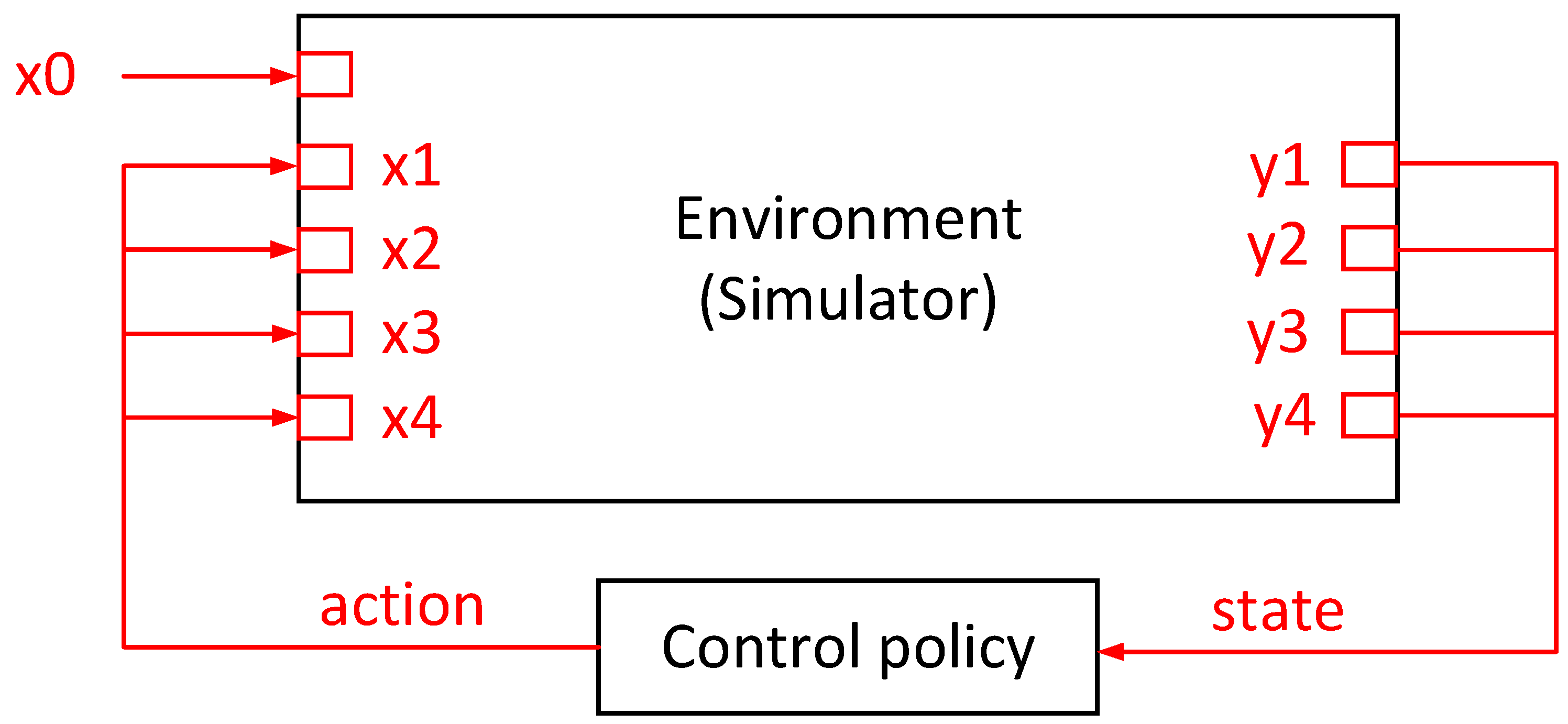
In this paper, the FIR filter was used to establish the transfer-function channels (i.e., the simulator) from the exciter and actuators to the sensors. Then, a reinforcement-learning algorithm interacted with the simulator to find a near-optimal control policy to meet the specified goals. Furthermore, the RL-based controller was verified in high-dimensional high-frequency vibration-control experiments.

The rest of this paper is organized as follow. First, the vibration-control problem is formulated. Second, a new method for a vibration-controller design through RL is presented. Third, the RL-designed vibration controller is experimentally verified. Finally, the conclusions are drawn.

2. Problem Formulation

Figure 1 shows the schematic diagram of the vibration-control system. The well-trained neural network is compiled into binary code, and it is then run on the controller hardware. The controller receives four acceleration signals from the sensors, and it outputs four control signals according to the control policy. Then, the control signals are sent to the four electromagnetic actuators to generate four control forces, which are expected to reduce the vibration in real time.

This is a high-dimensional high-frequency vibration-control problem. Our goal was to design an effective controller through reinforcement learning that can reduce vibrations under different vibration excitations.

3. Method

3.1. Method Overview

First, as shown in Figure 2, a simulator was built for the vibration system with an FIR filter. The vibration system has 5 inputs and 4 outputs. The 5 inputs refer to the forces of the vibration exciter and 4 electromagnetic actuators. The 4 outputs refer to the 4 acceleration signals. In detail, we used experimental data to identify an FIR filter, which acted as the simulator. We gave specified force signals to the vibration exciter and electromagnetic actuators, which applied forces to the vibration system. Both the force signals and corresponding acceleration signals were recorded and used to identify the FIR filter.

Then, an RL algorithm collected data and found a control policy through the interaction with an environment, as shown in Figure 3. The simulator, which had enough physical fidelity, was used to describe the evolution of the acceleration signals. The RL algorithm used the collected simulator data to find a near-optimal policy with respect to the specified reward function.

Many RL algorithms have been presented to solve the optimal solution, including value-based algorithms, such as the DQN [29], DDQN [30], prioritized DDQN [31], dueling DDQN [32], distributional DQN [33], noisy DQN [34] and Rainbow [35] algorithms. These value-based algorithms are suitable for problems with discrete and low-dimensional action spaces, such as electronic games, and therefore they were not used in this work. The DDPG [36] algorithm was chosen for the vibration control in this work, as it is suitable for high-dimensional continuous-action spaces. The DDPG is a model-free off-policy actor–critic algorithm that uses deep networks and that can learn the control policy. The representation of the control policy of the actor is restricted, as it must run on hardware with real-time guarantees. Therefore, we used a fast five-layer feed-forward neural network in the actor. The actor was trained by the PyTorch software package.

Finally, the control policy was bundled with the associated experiment control targets into an executable using a compiler tailored towards real-time control at 1 kHz. The deterministic nature of the DDPG gives a deterministic policy to execute on the plant. Although the actor is trained by the PyTorch software package, the well-trained actor is rewritten by the Simulink and NI/Veristand software packages, where the NI/Veristand acts as a plug-in of Simulink. The actor written in Simulink is then compiled into binary code. Finally, the binary code is run on the NI controller hardware.

3.2. Vibration-System Simulator

3.2.1. FIR Filter

An adaptive FIR filter was used for building the simulator. As shown in Figure 4, in order to implement an FIR filter, the input signal ($x\left(n\right)$) and desired output signal ($d\left(n\right)$) should be given. Note that the $x\left(n\right)$ and $d\left(n\right)$ are both vectors:

$$x\left(\mathrm{n}\right)={\left[x\left(n\right) x\left(n-1\right) \cdots x\left(x-N+1\right)\right]}^T$$

(1)

$$d\left(\mathrm{n}\right)={\left[d\left(n\right) d\left(n-1\right) \cdots d\left(x-N+1\right)\right]}^T$$

(2)

where N is the length of the filter. The given input signal ($x\left(n\right)$) of the filter is known, and the filter output signal ($\mathrm{y}\left(n\right)$) is formulated as:

$$\mathrm{y}\left(n\right)={\omega }^T\left(n\right)x\left(\mathrm{n}\right)$$

(3)

where n indicates the time sequence, and $\omega \left(n\right)$ is the vector of the filter weights.

The output signal ($\mathrm{y}\left(n\right)$) is the estimate of the desired signal ($d\left(n\right)$). The error ($e\left(n\right)$) between the output signal ($\mathrm{y}\left(n\right)$) and desired output signal ($d\left(n\right)$) is defined as:

$$e\left(n\right)=d\left(n\right)-y\left(n\right)$$

(4)

We estimate the filter weights ($\omega \left(n\right)$) to minimize the error ($e\left(n\right)$) by using the least-mean-square (LMS) algorithm [37]:

$$\omega \left(n+1\right)=\omega \left(n\right)+2\mu e\left(n\right)x\left(n\right)$$

(5)

where $\mu$ is the step size.

The filter weights ($\omega \left(n\right)$) can be easily well estimated if the appropriate input signal ($x\left(n\right)$) and desired output signal ($d\left(n\right)$) are given. In this work, the input signal and desired output signal are the experimental data.

3.2.2. Simulator Established with FIR Filter

The simulator can be considered as a 5-input/4-output filter. The input signals are denoted as $x_0\left(n\right)$, $x_1\left(n\right)$,$x_2\left(n\right)$,$x_3\left(n\right)$and $x_4\left(n\right)$, where $x_0\left(n\right)$ stands for the force signal of the vibration exciter, and $x_1\left(n\right)$,$x_2\left(n\right)$,$x_3\left(n\right)$,$x_4\left(n\right)$ stand for the force signals of the 4 electromagnetic actuators. The desired-output signals are denoted as $d_1\left(n\right)$,$d_2\left(n\right)$,$d_3\left(n\right)$,$d_4\left(n\right)$, which stand for the acceleration signals. Moreover, $y_j\left(n\right)$ is the estimate of the desired output ($d_j\left(n\right)$,$j=1,2,3,4$).

Obviously, there are $5\times 4=20$ channels between the inputs and desired outputs. Each channel can be expressed by an FIR filter. It is assumed that the symbol $C_{ij}$ stands for the filter between $x_i\left(n\right)$ and$d_j\left(n\right)$, where $i=0,1,2,3,4$ and $j=1,2,3,4$.

Note that $d_1\left(n\right)$ is the open-loop response under excitations of $x_0\left(n\right)$, $x_1\left(n\right)$,$x_2\left(n\right)$,$x_3\left(n\right)$,$x_4\left(n\right)$. Thus, the estimate of $d_1\left(n\right)$ can be formulated as follows:

$$\begin{gathered} y_1\left(n\right)={\omega }_{01}^T\left(n\right)x_0\left(n\right)+{\omega }_{11}^T\left(n\right)x_1\left(n\right)+{\omega }_{21}^T\left(n\right)x_2\left(n\right)+ \\ {\omega }_{31}^T\left(n\right)x_3\left(n\right)+{\omega }_{41}^T\left(n\right)x_4\left(n\right) \end{gathered}$$

(6)

where $y_1\left(n\right)$ is the estimate of $d_1\left(n\right)$, and ${\omega }_{i1}\left(n\right)$are the filter weights of filter $C_{i1}$. It can be found that $y_1\left(n\right)$ is the superposition of the outputs of 5 FIR filters. Similarly, the estimates of $d_2\left(n\right)$,$d_3\left(n\right)$,$d_4\left(n\right)$ are formulated as:

$$\begin{gathered} y_2\left(n\right)={\omega }_{02}^T\left(n\right)x_0\left(n\right)+{\omega }_{12}^T\left(n\right)x_1\left(n\right)+{\omega }_{22}^T\left(n\right)x_2\left(n\right)+ \\ {\omega }_{32}^T\left(n\right)x_3\left(n\right)+{\omega }_{42}^T\left(n\right)x_4\left(n\right) \end{gathered}$$

(7)

$$\begin{gathered} y_3\left(n\right)={\omega }_{03}^T\left(n\right)x_0\left(n\right)+{\omega }_{13}^T\left(n\right)x_1\left(n\right)+{\omega }_{23}^T\left(n\right)x_2\left(n\right)+ \\ {\omega }_{33}^T\left(n\right)x_3\left(n\right)+{\omega }_{43}^T\left(n\right)x_4\left(n\right) \end{gathered}$$

(8)

$$\begin{gathered} y_4\left(n\right)={\omega }_{04}^T\left(n\right)x_0\left(n\right)+{\omega }_{14}^T\left(n\right)x_1\left(n\right)+{\omega }_{24}^T\left(n\right)x_2\left(n\right)+ \\ {\omega }_{34}^T\left(n\right)x_3\left(n\right)+{\omega }_{44}^T\left(n\right)x_4\left(n\right) \end{gathered}$$

(9)

Equations (6)–(9) can be written in the compact form of Equation (10), which is the simulator of the vibration system:

$$y\left(n\right)=W\left(n\right)X\left(n\right)$$

(10)

where

$$\begin{gathered} y\left(n\right)={\left[\begin{array}{ccc}{y}_1\left(n\right)& y_2\left(n\right)& \begin{array}{cc}{y}_3\left(n\right)& y_4\left(n\right)\end{array}\end{array}\right]}^T \\ X\left(n\right)={\left[\begin{array}{ccc}{x}_0^T\left(n\right)& x_1^T\left(n\right)& \begin{array}{ccc}{x}_2^T\left(n\right)& x_3^T\left(n\right)& x_4^T\left(n\right)\end{array}\end{array}\right]}^T \\ W\left(n\right)=\left[\begin{array}{ccc}\begin{array}{c}{\omega }_{01}^T\left(n\right)\\ {\omega }_{02}^T\left(n\right)\\ \begin{array}{c}\cdots \\ {\omega }_{04}^T\left(n\right)\end{array}\end{array}& \begin{array}{c}\begin{array}{cc}{\omega }_{11}^T\left(n\right)& \cdots \end{array}\\ \begin{array}{cc}{\omega }_{13}^T\left(n\right)& \cdots \end{array}\\ \begin{array}{cc}\begin{array}{c}\cdots \\ {\omega }_{14}^T\left(n\right)\end{array}& \begin{array}{c}\cdots \\ \cdots \end{array}\end{array}\end{array}& \begin{array}{c}{\omega }_{41}^T\left(n\right)\\ {\omega }_{42}^T\left(n\right)\\ \begin{array}{c}\cdots \\ {\omega }_{44}^T\left(n\right)\end{array}\end{array}\end{array}\right] \end{gathered}$$

The simulator is composed of 20 single-input/single-output filters. The matrix ($W\left(n\right)$) contains the filter weights of the 20 filters, where ${\omega }_{ij}\left(n\right)$is the vector of the weights of filter $C_{ij}$: $i=0,1,2,3,4$ and $j=1,2,3,4$.

3.2.3. Estimate of Simulator Weights

The simulator can be considered as a 5-input/4-output filter. We estimated the simulator weights and validated the physical fidelity of the simulator. Because the simulator is composed of 20 single-input/single-output filters, the weights of the 20 filters can be estimated independently. Without losing generality, we take filters $C_{4j}$,$j=1,2,3,4$ as examples to show how to estimate the filter weights and validate the filters.

We turned on the No. 4 actuator and left the other actuators and the vibration exciter off. A narrow-band random white-noise signal, shown in Figure 5, was used as the input signal $x_4\left(\mathrm{n}\right)$, and then the signals of the acceleration sensors were collected ($d_1\left(n\right)$,$d_2\left(n\right)$,$d_3\left(n\right)$,$d_4\left(n\right)$). Because only the No. 4 actuator was turned on, $x_0\left(n\right)$, $x_1\left(n\right)$,$x_2\left(n\right)$,$x_3\left(n\right)$ were zeros, and so Equations (6)–(9) were simplified as follows:

$$y_1\left(n\right)={\omega }_{41}^T\left(n\right)x_4\left(n\right)$$

(11)

$$y_2\left(n\right)={\omega }_{42}^T\left(n\right)x_4\left(\mathrm{n}\right)$$

(12)

$$y_3\left(n\right)={\omega }_{43}^T\left(n\right)x_4\left(n\right)$$

(13)

$$y_4\left(n\right)={\omega }_{44}^T\left(n\right)x_4\left(n\right)$$

(14)

According to Equation (5), the filter weights (${\omega }_{41}\left(n\right)$, ${\omega }_{42}\left(n\right)$, ${\omega }_{43}\left(n\right)$, ${\omega }_{44}\left(n\right)$) can be obtained.

It is known that $y_j\left(n\right)$ is the estimate of the desired output ($d_j\left(n\right)$,$j=1,2,3,4$). The desired outputs and their estimates by FIR filters are compared in Figure 6. The normalized mean square error (NMSE) [38] was used to evaluate the estimate precision. The NMSEs were all smaller than 20%, which shows that the desired outputs were well estimated, and the filters were validated. It also means that the simulator shown in Equation (10) had enough physical fidelity to describe the vibration system.

The definition of the NMSE is formulated by:

$$\mathrm{NMSE}=\frac{\Vert d_j\left(n\right)-y_j\left(n\right){\Vert }^2}{\Vert d_j\left(n\right)-mean\left(d_j\left(n\right)\right){\Vert }^2}$$

(15)

where ‖⬚‖ indicates the 2-norm of a vector.

Next, the other filters can be estimated and validated in a similar way. For instance, we turned on the vibration exciter and left the actuators off, and we gave the same signal shown in Figure 5 to the vibration exciter. The filter weights (${\omega }_{01}\left(n\right)$, ${\omega }_{02}\left(n\right)$, ${\omega }_{03}\left(n\right)$, ${\omega }_{04}\left(n\right)$) could be obtained. It should be noted that the simulator can only well estimate the outputs of the vibration system when the input forces are from 50 Hz to 60 Hz.

3.3. Control Policy by Reinforcement Learning

3.3.1. Learning Loop

The control policy is learned through reinforcement learning. The RL algorithm collects simulator data and finds a control policy through the interaction with an environment. The episode-training approach is used, in which data are collected by running the simulator with a control policy in the loop, as shown in Figure 3. The data from these interactions are collected in a finite-capacity first-in/first-out buffer. The interaction trajectories are sampled from the buffer by a ‘learner’, which executes the DDPG algorithm to update the control-policy parameters. The details of the training loop are introduced in the following sections.

3.3.2. State Space and Action Space

In Figure 3, the state space is composed of the acceleration signals. The state space is formulated by:

$$s={\left[\begin{array}{ccc}{y}_1^T\left(n\right)& y_2^T\left(n\right)& \begin{array}{cc}{y}_3^T\left(n\right)& y_4^T\left(n\right)\end{array}\end{array}\right]}^T$$

(16)

where n indicates the time sequence, and $y_1^T\left(n\right)$,$y_2^T\left(n\right)$,$y_3^T\left(n\right)$,$y_4^T\left(n\right)$ are the outputs of the simulator. It is known that:

$$y_j\left(\mathrm{n}\right)={\left[\begin{array}{ccc}{y}_j\left(n\right)& y_j\left(n-1\right)& \begin{array}{cc}\cdots & y_j\left(x-N+1\right)\end{array}\end{array}\right]}^T$$

(17)

where $j=1,2,3,4$, and N is the length of the filter. In this work, N=50, and so the space state is the vector that contains 200 elements.

The action space is composed of the force signals of the actuators. The action space is formulated by:

$$a={\left[\begin{array}{ccc}{x}_1\left(n\right)& x_2\left(n\right)& \begin{array}{cc}{x}_3\left(n\right)& x_4\left(n\right)\end{array}\end{array}\right]}^T$$

(18)

where $x_1\left(n\right)$,$x_1\left(n\right)$,$x_1\left(n\right)$,$x_1\left(n\right)$ are the inputs of the simulator. The space state is the vector that contains 4 elements.

3.3.3. Reward

On the one hand, in reinforcement learning, the goal of the control policy is to interact with the simulator by selecting actions in a way that maximizes future rewards. On the other hand, the goal of vibration control is to minimize the accelerations. Therefore, for each time step, the reward is defined by:

$$r\left(n\right)=-\left(y_1^2\left(n\right)+y_2^2\left(n\right)+y_3^2\left(n\right)+y_4^2\left(n\right)\right)$$

(19)

where n indicates the time sequence, and $y_1\left(n\right)$,$y_2\left(n\right)$,$y_3\left(n\right)$,$y_4\left(n\right)$ are the output acceleration signals of the simulator.

In general, we seek to maximize the expected return, where the return is defined as the sum of the discounted rewards [39]:

$$\mathrm{G}\left(n\right)=r\left(n\right)+\gamma r\left(n+1\right)+{\gamma }^2 r\left(n+2\right)+\cdots +{\gamma }^T r\left(n+T\right)$$

(20)

where T is the final time step, and $\mathsf{\gamma }$ is the parameter$0\le \mathsf{\gamma }\le 1$, which is called the discount rate. In this work, $\gamma =1$.

3.3.4. Neural-Network Architecture

DDPG uses two neural-network architectures to design and optimize the policy: the critic network and policy network. Both networks are updated during training, but only the policy network is deployed on the plant.

The critic network is a five-layer feed-forward neural network that contains three hidden layers with 200 neurons each. The state space and action space are the input data to be fed into the input layer. For each hidden layer, the activation function, the hyperbolic-tangent function, is used. A last linear layer is used to output the Q-value.

The policy network is also a five-layer feed-forward neural network. It deterministically maps states to specific actions. The input layer represents the space state, and the output layer represents the action space. Each of the three hidden layers has 200 neurons and is activated by the hyperbolic-tangent function.

3.3.5. Learning Curve

The training loop has been defined in detail. The vibration-exciter input should be given to the simulator before starting training. The narrow-band random white-noise signal from 50 Hz to 60 Hz, shown in Figure 5, is used as the vibration-exciter input. The controller controls the actuators to reduce the vibration caused by the exciter. The learning curve, shown in Figure 7, shows the return of each training episode. Each episode has the same length of 1 × 10⁵ time steps, and the simulation time step is 0.001 s. The return is defined by Equation (19). At the end of each episode, the control policy is updated. The learning curve shows that the control policy converges to a near-optimal point after about 60 training episodes.

3.4. Simulation of the Control Performance

After the control policy was well trained, we tested the control policy by vibration-control simulations. Figure 8 shows the vibration-control-simulation architecture. The control policy, the parameters of which are fixed, and the simulator are used together for the vibration-control simulations.

We carried out many simulations with different excitation signals. The simulation results show that the control policy can effectively reduce vibrations from 50 Hz to 60 Hz. For clarity, one simulation case was chosen to be shown.

Simulation #1

A superposition signal of 52 Hz, 55 Hz and 58 Hz sinuous signals was given to the vibration exciter. The control policy controls the actuators to reduce the vibration caused by the exciter. We simulated and compared the simulator sensor responses with or without control. The simulation time was as long as 30 s. For clarity, a short time span of 0.5 s is shown.

Figure 9 shows the sensor signals in the time domain. The root-mean-square (RMS) value was used to evaluate the sensor signals. A smaller RMS value generally means a weaker vibration.

Table 1. RMS values of sensor signals: Simulation #1.

	Uncontrolled (V)	Controlled (V)	Reduction (%)
No. 1 Sensor	0.1060	0.0449	57.65%
No. 2 Sensor	0.0880	0.0482	45.21%
No. 3 Sensor	0.0541	0.0231	57.36%
No. 4 Sensor	0.1269	0.0646	49.10%

shows the RMS values of the uncontrolled and controlled sensor signals. It was found that the RMS values were all reduced by more than 45%.

The vibration reduction can also be seen from the PSD curves of the sensor signals, as shown in Figure 10.

Table 2. Peak values of PSD curves of sensor signals: Simulation #1.

		Uncontrolled (V2/Hz)	Controlled (V2/Hz)	Reduction (%)
	@52 Hz	0.0297	0.0035	88.24%
No. 1 Sensor	@55 Hz	0.0190	0.0034	82.13%
	@58 Hz	0.0063	0.0023	63.95%
	@52 Hz	0.0187	0.0051	72.77%
No. 2 Sensor	@55 Hz	0.0137	0.0037	73.18%
	@58 Hz	0.0055	0.0021	62.24%
	@52 Hz	0.0089	0.0006	93.71%
No. 3 Sensor	@55 Hz	0.0044	0.0016	63.97%
	@58 Hz	0.0010	0.0003	74.42%
	@52 Hz	0.0409	0.0098	75.95%
No. 4 Sensor	@55 Hz	0.0272	0.0055	79.64%
	@58 Hz	0.0106	0.0038	64.15%

shows the peak values of the PSD curves of the sensor signals. It can be seen that the peak values of the PSD curves at specific frequencies were all reduced by more than 63%. Moreover, Figure 11 shows that the neural-network outputs were bounded from −2 V to 2 V.

4. Experiment

4.1. Experimental Setup and Procedure

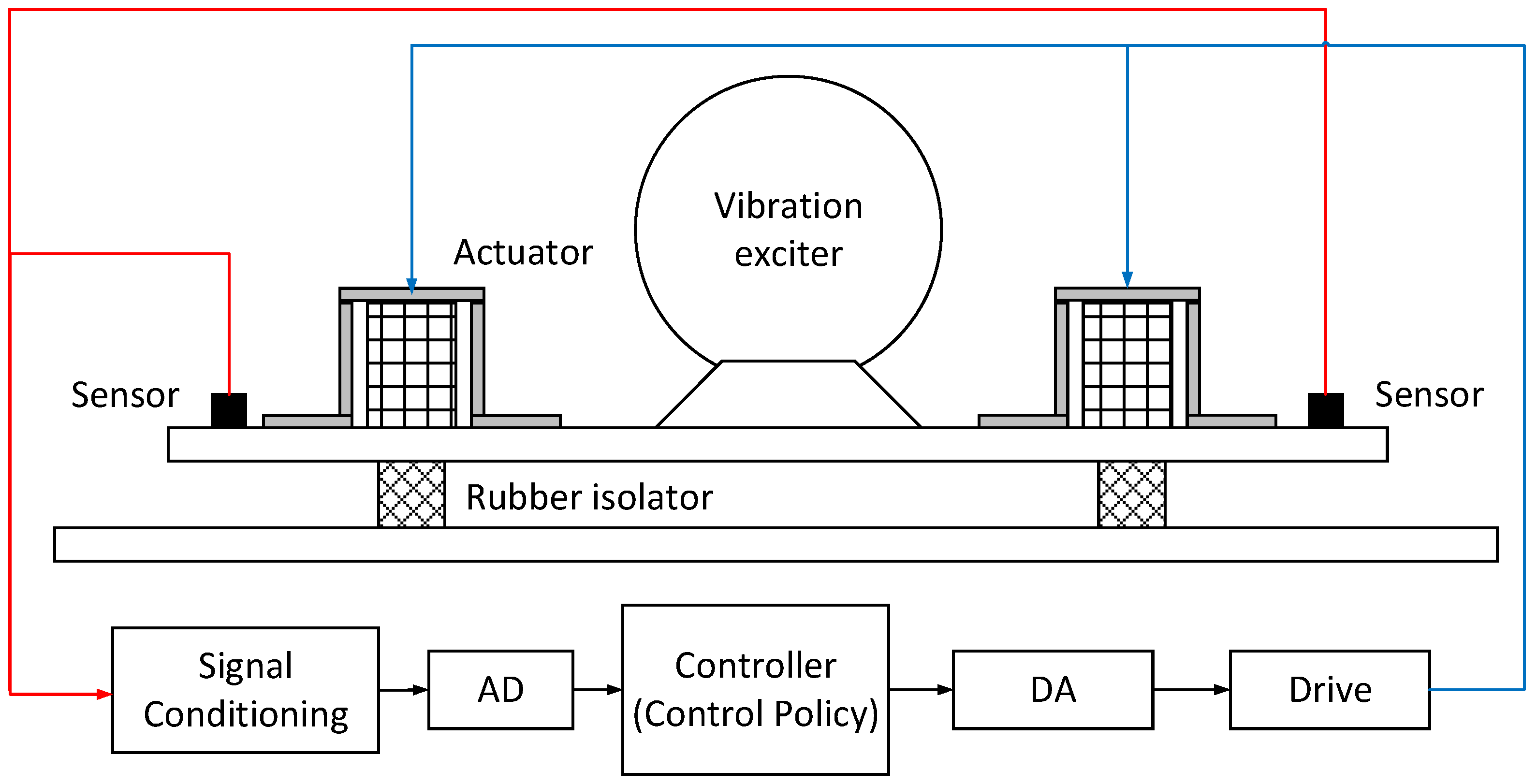
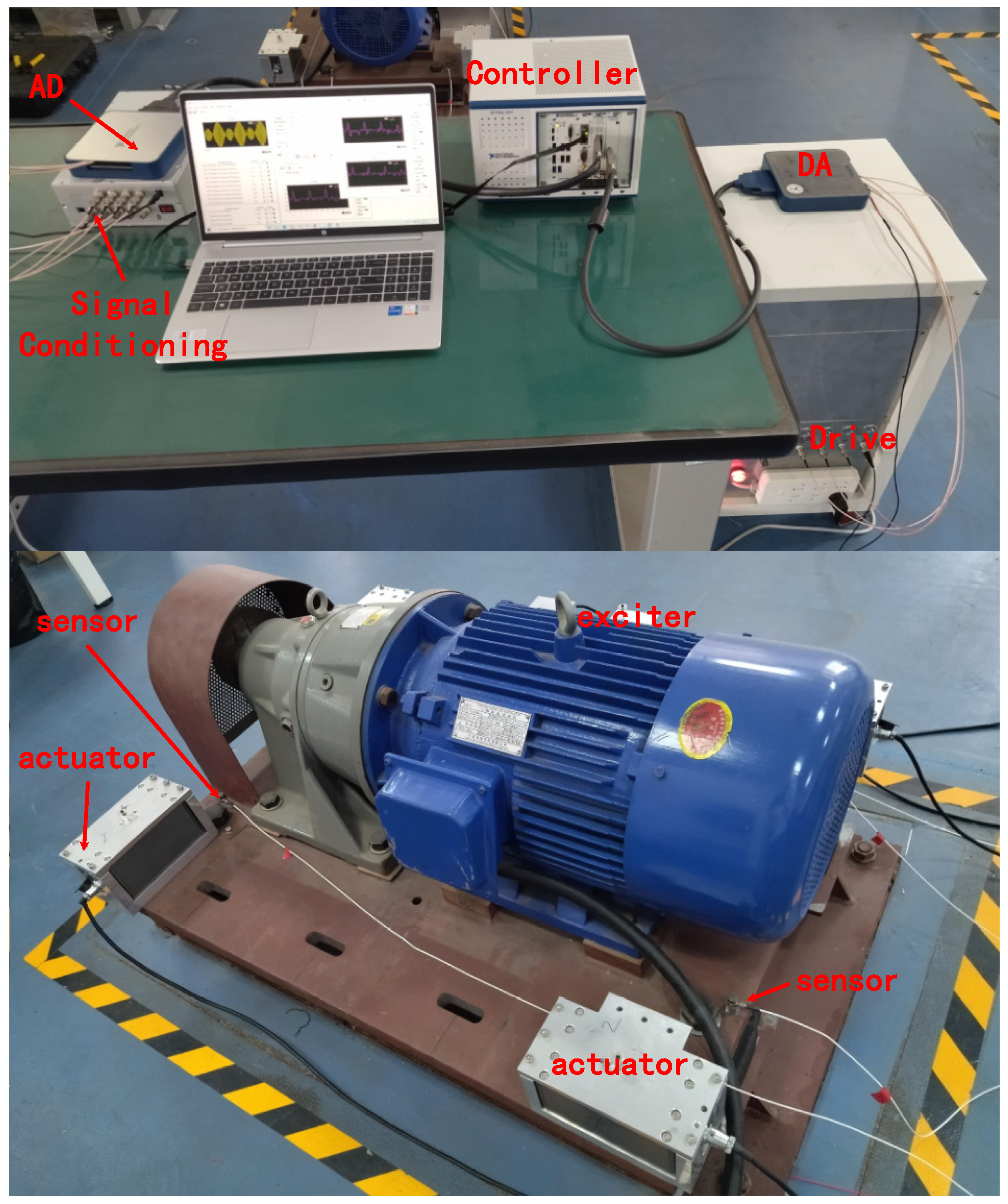
As shown in Figure 12, the vibration system was supported on the ground by rubber isolators. A vibration exciter was installed on the vibration system to generate the vibration-excitation force. The control system includes the acceleration sensors, signal-conditioning module, AD module, controller, DA module, drive module and electromagnetic actuators. The acceleration sensors measure the system vibration. The well-trained neural network is compiled into binary code, and it is then run on the controller hardware. The controller controls the electromagnetic actuators to reduce the vibration caused by the exciter.

We carried out many different experiments by giving different signals to the vibration exciter. For clarity, three experiments were chosen to be shown.

In Experiment #1, the signal given to the exciter is the superposition of the 52 Hz, 55 Hz and 58 Hz sine signals, and it is the same as that in Simulation #1.

In Experiment #2, the signal given to the exciter is the superposition of the 53 Hz, 56 Hz and 59 Hz sine signals.

In Experiment #3, the signal given to the exciter is the superposition of the 53 Hz, 56 Hz, and 59 Hz sine signals, but its amplitude is completely different from that in Experiment #2.

The parameters of the well-trained neural network were fixed in all the experiments. The controller controls the actuators to reduce the vibration caused by the exciter. In each experiment, the sensor signals were recorded when the controller was turned on or off. Some of the experimental results were chosen to be shown in the following sections.

4.2. Experimental Results and Discussions

4.2.1. Experiment #1

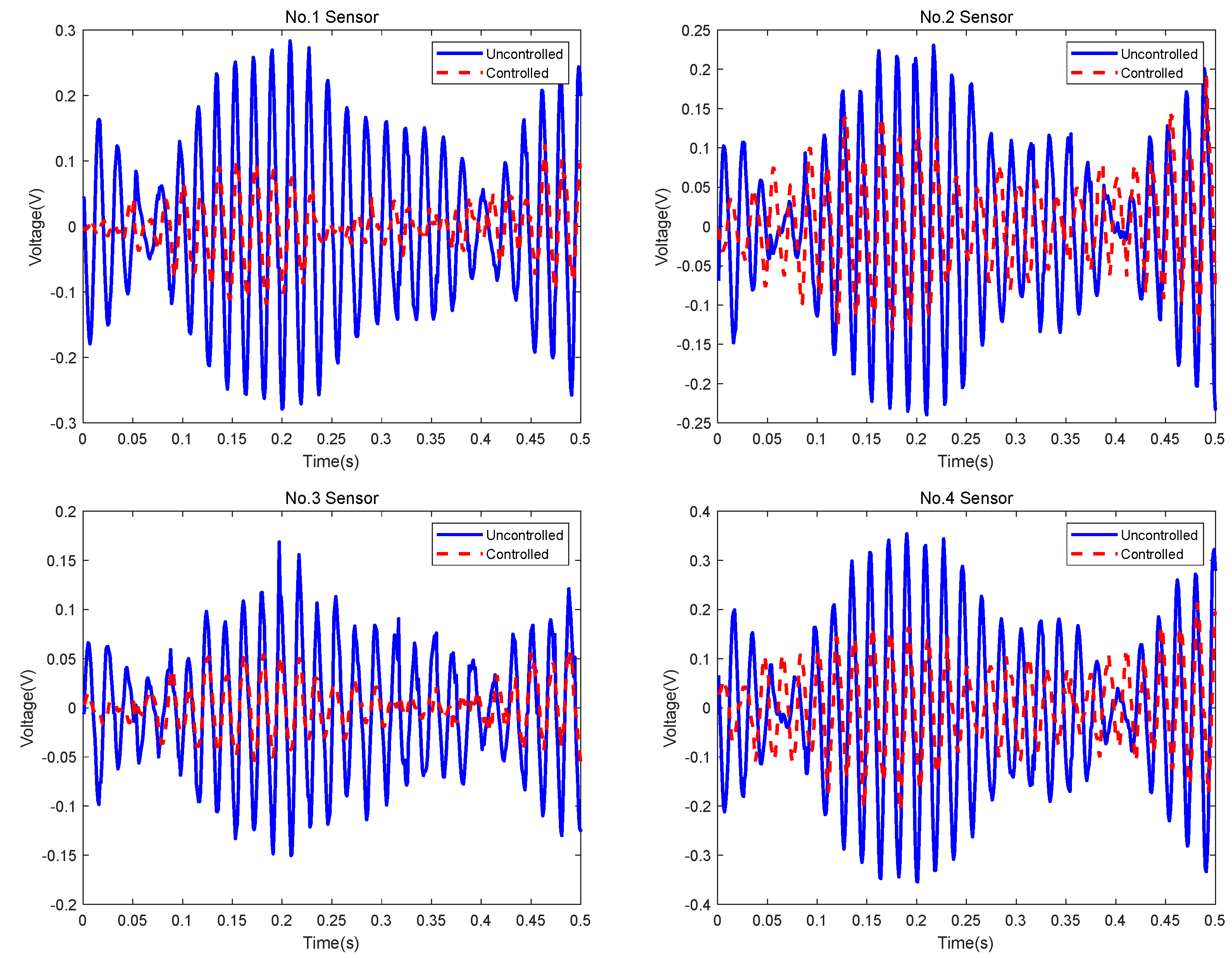
Figure 13 shows the sensor signals in the time domain. The controlled signals were recorded when the controller was on, and the uncontrolled signals were recorded when the controller was off. Although the controlled signals and uncontrolled signals are shown in the same figure, they were not sampled at the same time. The sampling frequency was 1 kHz. The amount of the total sampled data was more than 30 s. For clarity, a small amount of data is shown in the figures.

Table 3. RMS values of sensor signals: Experiment #1.

	Uncontrolled (V)	Controlled (V)	Reduction (%)
No. 1 Sensor	0.1303	0.0439	66.26%
No. 2 Sensor	0.1060	0.0644	39.23%
No. 3 Sensor	0.0655	0.0237	63.78%
No. 4 Sensor	0.1625	0.0885	45.52%

shows the RMS values of the uncontrolled and controlled sensor signals. The RMS values were calculated based on the total sampled data. It was found that the RMS values were reduced by more than 39%. The vibration reduction can also be seen from the PSD curves of the sensor signals, as shown in Figure 14.

Table 4. Peak values of PSD curves of sensor signals: Experiment #1.

		Uncontrolled (V2/Hz)	Controlled (V2/Hz)	Reduction (%)
	@52 Hz	0.0520	0.0031	94.04%
No. 1 Sensor	@55 Hz	0.0209	0.0030	85.75%
	@58 Hz	0.0067	0.0020	66.93%
	@52 Hz	0.0302	0.0088	70.83%
No. 2 Sensor	@55 Hz	0.0156	0.0047	69.82%
	@58 Hz	0.0060	0.0032	47.49%
	@52 Hz	0.0142	0.0008	94.53%
No. 3 Sensor	@55 Hz	0.0040	0.0013	68.00%
	@58 Hz	0.0009	0.0002	72.66%
	@52 Hz	0.0747	0.0169	77.36%
No. 4 Sensor	@55 Hz	0.0372	0.0092	75.24%
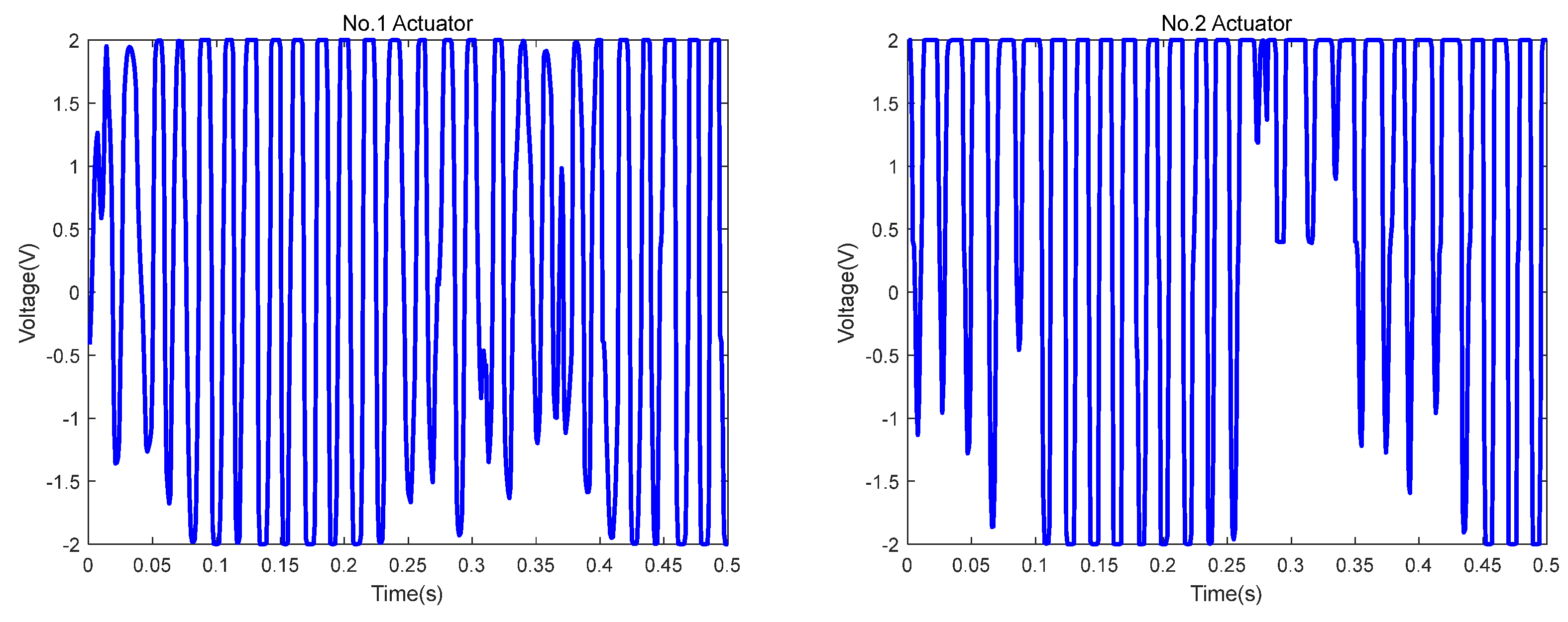
	@58 Hz	0.0133	0.0062	53.19%

shows the peak values of the PSD curves of the sensor signals. It can be seen that the peak values of the PSD curves at specific frequencies were reduced by more than 47%. Moreover, Figure 15 shows that the controller outputs were bounded from −2 V to 2 V.

4.2.2. Experiment #2

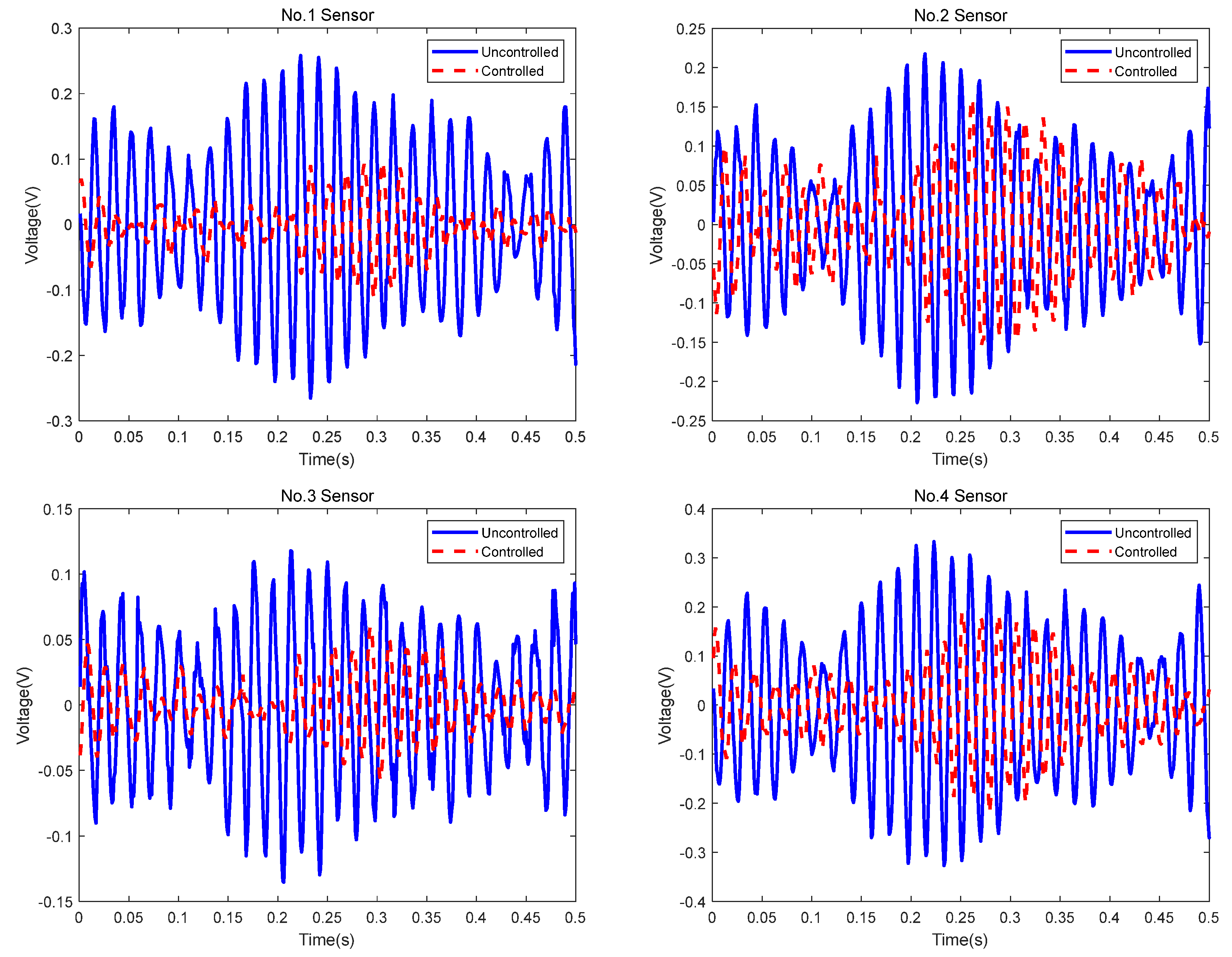
Figure 16 shows the sensor signals in the time domain.

Table 5. RMS values of sensor signals: Experiment #2.

	Uncontrolled (V)	Controlled (V)	Reduction (%)
No. 1 Sensor	0.1290	0.0392	69.60%
No. 2 Sensor	0.1070	0.0632	40.94%
No. 3 Sensor	0.0616	0.0220	64.35%
No. 4 Sensor	0.1641	0.0799	51.32%

shows the RMS values of the uncontrolled and controlled sensor signals. It was found that the RMS values were all reduced by more than 40%. The vibration reduction can also be seen from the PSD curves of the sensor signals, as shown in Figure 17.

Table 6. Peak values of PSD curves of sensor signals: Experiment #2.

		Uncontrolled (V2/Hz)	Controlled (V2/Hz)	Reduction (%)
	@53 Hz	0.0605	0.0027	95.47%
No. 1 Sensor	@56 Hz	0.0127	0.0021	83.41%
	@59 Hz	0.0050	0.0017	65.36%
	@53 Hz	0.0385	0.0096	74.96%
No. 2 Sensor	@56 Hz	0.0100	0.0046	54.58%
	@59 Hz	0.0046	0.0034	24.59%
	@53 Hz	0.0141	0.0010	92.88%
No. 3 Sensor	@56 Hz	0.0021	0.0009	59.92%
	@59 Hz	0.0006	0.0002	68.66%
	@53 Hz	0.0942	0.0154	83.61%
No. 4 Sensor	@56 Hz	0.0235	0.0089	62.31%
	@59 Hz	0.0101	0.0050	50.38%

shows the peak values of the PSD curves of the sensor signals. It can be seen that the peak values of the PSD curves at specific frequencies were nearly all reduced by more than 50%.

4.2.3. Experiment #3

Figure 18 shows the sensor signals in the time domain.

Table 7. RMS values of PSD curves of sensor signals: Experiment #3.

	Uncontrolled (V)	Controlled (V)	Reduction (%)
No. 1 Sensor	0.0875	0.0394	55.02%
No. 2 Sensor	0.0767	0.0422	44.98%
No. 3 Sensor	0.0425	0.0203	52.28%
No. 4 Sensor	0.1139	0.0773	32.10%

shows the RMS values of the uncontrolled and controlled sensor signals. It was found that the RMS values were all reduced by more than 32%. The vibration reduction can also be seen from the PSD curves of the sensor signals, as shown in Figure 19.

Table 8. Peak values of PSD curves of sensor signals: Experiment #3.

		Uncontrolled (V2/Hz)	Controlled (V2/Hz)	Reduction (%)
	@53 Hz	0.0099	0.0007	92.65%
No. 1 Sensor	@56 Hz	0.0121	0.0012	90.39%
	@59 Hz	0.0138	0.0029	79.31%
	@53 Hz	0.0061	0.0017	72.52%
No. 2 Sensor	@56 Hz	0.0092	0.0017	81.76%
	@59 Hz	0.0122	0.0041	66.49%
	@53 Hz	00032	0.00008	97.55%
No. 3 Sensor	@56 Hz	0.0027	0.0001	95.78%
	@59 Hz	0.0021	0.0002	90.00%
	@53 Hz	0.0129	0.0049	61.80%
No. 4 Sensor	@56 Hz	0.0191	0.0049	74.47%
	@59 Hz	0.0244	0.0116	52.53%

shows the peak values of the PSD curves of the sensor signals. It can be seen that the peak values of the PSD curves at specific frequencies were all reduced by more than 52%.

4.3. Comparison of Experimental and Simulation Results

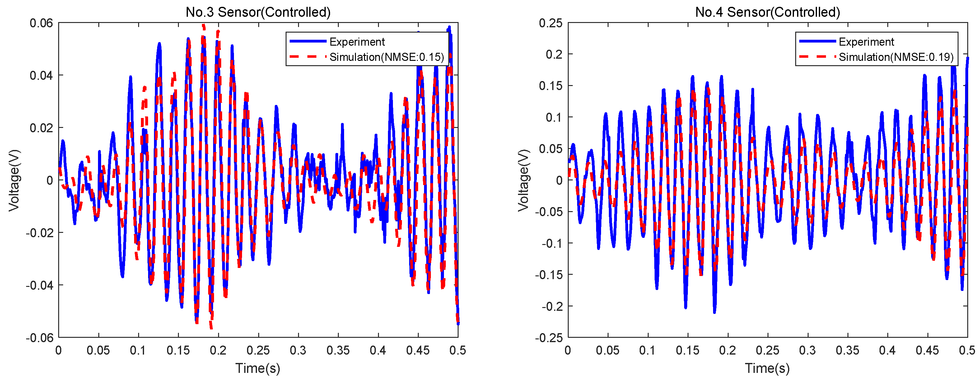
The results of Simulation #1 and Experiment #1 were compared. The physical fidelity of the simulation model, including the simulator and control policy, was validated.

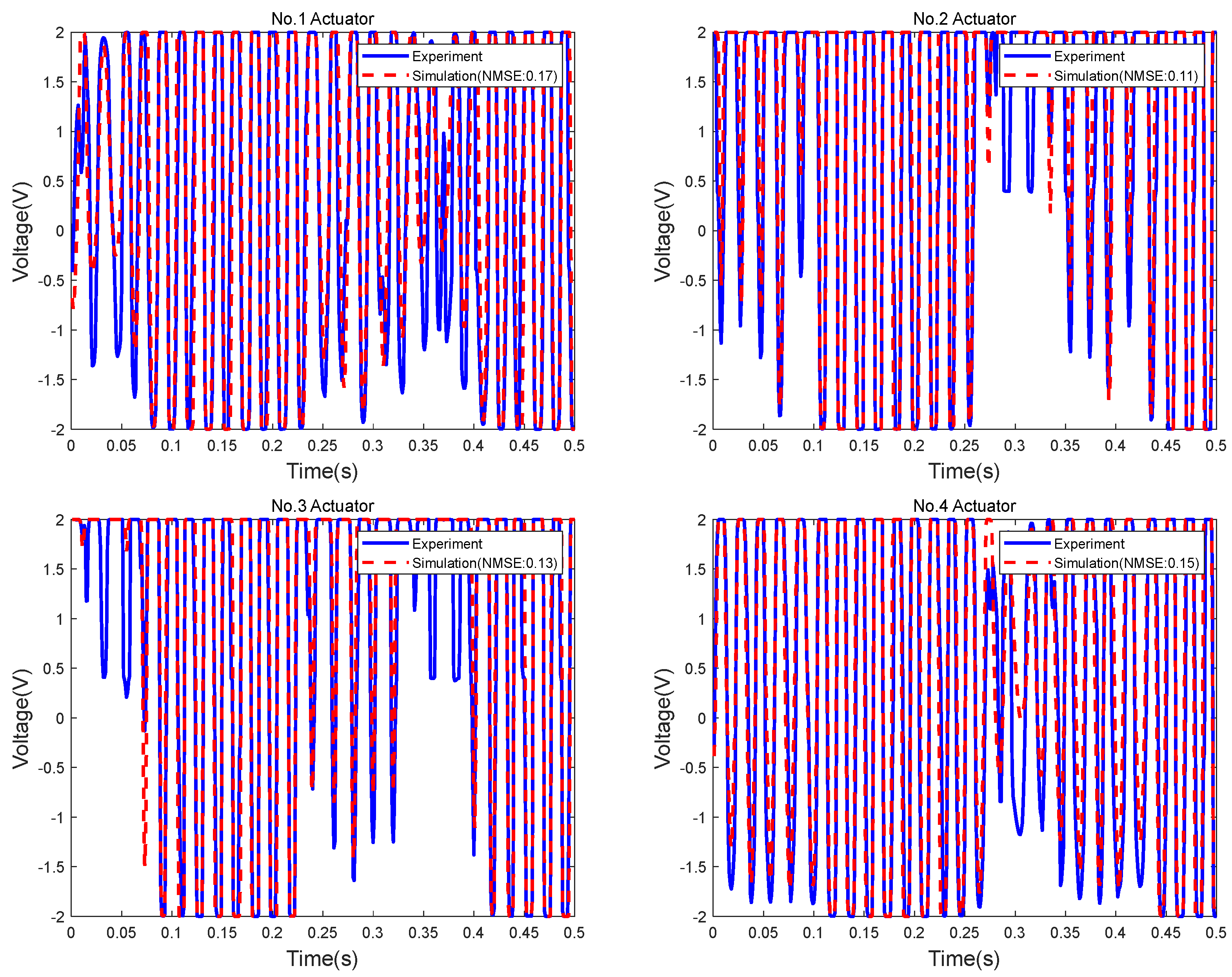
Figure 20 shows the sensor signals obtained by the simulation and experiment. The NMSEs between the experimental and simulation signals from the No. 1 to No. 4 sensors are 14%, 17%, 15% and 19%, respectively. Figure 21 shows the actuator signals obtained by the simulation and experiment. The NMSEs between the experimental and simulation signals from the No. 1 to No. 4 actuators are 17%, 11%, 13% and 15%, respectively.

The errors mainly come from the errors between the real-world vibration system and the simulator, the time delay and signal interference of the electronic components, external disturbances, and so on. However, the errors can be accepted. On the one hand, the errors are smaller than 20%, which can be accepted in most engineering problems. On the other hand, the experiment results also show that the simulation model has enough physical fidelity, and the proposed method for designing the vibration controller is effective and useful.

5. Control-Performance Verification

In order to further verify the effectiveness of the simulator established with the FIR filter, we carried out experiments based on another simulator that was established with dynamics equations. We set up the dynamics equations in the simulation software and trained the proposed RL-based controller, which interacted with the dynamics equations to find the optimal control policy, which was then used in the experiments.

The vibration system shown in Figure 22 is simplified as a spring–mass–damper system, which can be formulated by ordinary differential equations. The spring–mass–damper system has three degrees of freedom, including vertical motion along the Z-axis, rotation motion along the X-axis, and rotation motion along the Y-axis. The symbol $F_{ci}\left(i=1,2,34\right)$ stands for the control force of the actuator, and $F_{bi}\left(i=1,2,34\right)$ stands for the force of the rubber isolator. The symbol F denotes the force of the exciter, and its location is determined by the coordinates$\left(x,y\right)$. The dynamics equations are obtained at the equilibrium position:

$$M\ddot{z}=F+{{\displaystyle \sum }}_{i=1}^4\left(F_{ci}+F_{bi}\right)$$

(21)

$$I_{xx}\ddot{\theta }=\left(F_{c2}+F_{c3}\right)L_1-\left(F_{c1}+F_{c4}\right)L_2+F·y$$

(22)

$$I_{yy}\ddot{\gamma }=\left(F_{c1}+F_{c2}\right)L_3-\left(F_{c3}+F_{c4}\right)L_4-F·x$$

(23)

where $z$ denotes the vertical displacement of the mass center; $\theta$ denotes the rotation angle along the X-axis; $\mathsf{\gamma }$ denotes the rotation angle along the Y-axis; $M$ denotes the mass; $I_{xx}$ and $I_{yy}$ denote the inertias.

Next, the proposed RL-based controller that interacts with the dynamics equations was trained to find the optimal control policy. Then, the control policy was compiled into binary code and run on the controller hardware in the experiment. We performed the experiments by giving different signals to the vibration exciter. The controlled sensor signals were recorded when the controller was on, and the uncontrolled sensor signals were recorded when the controller was off.

Figure 23 shows the sensor signals when a simple 55 Hz sine signal was given to the exciter. The sampling frequency was 1 kHz. The amount of the total sampled data was more than 30 s. For clarity, a small amount of data is shown.

Table 9. RMS values of sensor signals.

	Uncontrolled (V)	Controlled (V)	Reduction (%)
No. 1 Sensor	0.0732	0.2140	−192.29%
No. 2 Sensor	0.1206	0.1852	−53.56%
No. 3 Sensor	0.0420	0.0948	−125.43%
No. 4 Sensor	0.1624	0.2753	−69.47%

shows the RMS values of the uncontrolled and controlled sensor signals. It was found that the RMS values were increased by more than 53%. The vibration enhancement can also be seen from the PSD curves of the sensor signals, as shown in Figure 24.

Table 10. Peak values of PSD curves of sensor signals.

		Uncontrolled (V2/Hz)	Controlled (V2/Hz)	Reduction (%)
No. 1 Sensor	@55 Hz	0.0248	0.2225	−797.05%
No. 2 Sensor	@55 Hz	0.0687	0.1650	−140.21%
No. 3 Sensor	@55 Hz	0.007	0.0419	−499.75%
No. 4 Sensor	@55 Hz	0.1264	0.3692	−192.00%

shows the peak values of the PSD curves of the sensor signals. It can be seen that the peak values of the PSD curves at specific frequencies were increased by more than 140%.

It was found that the control policy obtained by using the dynamics equations led to the vibration enhancement. In comparison with the control policy obtained by using the FIR filter, which effectively reduces the vibration, the effectiveness of the FIR filter could be verified.

The main reason for the vibration enhancement may be that the dynamics equations can only be used to effectively solve vibration-control problems of low dimension and simple dynamics. The parameters of the dynamic model were carefully verified, such as the mass, stiffness, damping, size, and so on, but it is still much less accurate than the FIR filter. Thus, it is difficult for the RL-based controller to successfully learn an effective control policy from the dynamics equations. To solve this problem, we present an RL-based controller that interacts with the accurate parametric model (FIR filter) instead of dynamics equations. Therefore, the RL-based controller converges more easily, and the vibration can be effectively reduced.

6. Conclusions

This paper presents an effective control method for solving high-dimensional high-frequency vibration-control problems based on reinforcement learning (RL) and a finite-impulse-response (FIR) filter. First, the FIR filter was used to build a simulator for the vibration system with five inputs (the forces of the vibration exciter and the four electromagnetic actuators) and four outputs (the four acceleration signals). Then, a reinforcement-learning algorithm interacted with the simulator to find a near-optimal control policy to meet the specified goals. Finally, the controller was validated by numerical simulations and experiments. The numerical results show that the peak values of the PSD curves at specific frequencies were maximumly reduced by more than 63%. The experimental results show that the controller can effectively reduce various vibrations (the peak values of the PSD curves maximumly reduced by more than 52%) within a frequency range from 50 Hz to 60 Hz. This means that we can provide an effective method to solve high-dimensional high-frequency vibrational-control problems.

In this work, the controller was designed and validated within a frequency range from 50 Hz to 60 Hz. In fact, the controller can be designed within a wider frequency range, such as a range from 10 Hz to 100 Hz. Generally, a larger neural network is needed for vibration control in a wider frequency range. Moreover, it will be much more difficult to train. Meanwhile, the controller hardware should be improved to guarantee the computation speed, as a larger network costs more computation resources. Our further work focuses on designing and training a complex neural-network architecture for a vibration controller in a wider frequency range. Meanwhile, we also have to update the hardware to achieve a faster computation speed.

References

1. Ab Talib, M.H.; Mat Darus, I.Z.; Mohd Samin, P.; Mohd Yatim, H.; Ardani, M.I.; Shaharuddin, N.M.R.; Hadi, M.S. Vibration control of semi-active suspension system using PID controller with advanced firefly algorithm and particle swarm optimization. J. Ambient. Intell. Hum. Comput. 2021, 12, 1119–1137. [Google Scholar] [CrossRef]
2. Li, W.; Yang, Z.; Li, K.; Wang, W. Hybrid feedback PID-FxLMS algorithm for active vibration control of cantilever beam with piezoelectric stack actuator. J. Sound Vib. 2021, 509, 116243. [Google Scholar] [CrossRef]
3. Wang, L.; Liu, J.; Yang, C.; Wu, D. A novel interval dynamic reliability computation approach for the risk evaluation of vibration active control systems based on PID controllers. Appl. Math. Model. 2021, 92, 422–446. [Google Scholar] [CrossRef]
4. Zhang, Q.; Yang, Z.; Wang, C.; Yang, Y.; Zhang, R. Intelligent control of active shock absorber for high-speed elevator car. Proc. Inst. Mech. Eng. Part C J. Mech. Eng. Sci. 2019, 233, 3804–3815. [Google Scholar] [CrossRef]
5. Tian, J.; Guo, Q.; Shi, G. Laminated piezoelectric beam element for dynamic analysis of piezolaminated smart beams and GA-based LQR active vibration control. Compos. Struct. 2020, 252, 112480. [Google Scholar] [CrossRef]
6. Takeshita, A.; Yamashita, T.; Kawaguchi, N.; Kuroda, M. Fractional-order LQR and state observer for a fractional-order vibratory system. Appl. Sci. 2021, 11, 3252. [Google Scholar] [CrossRef]
7. Lu, X.; Liao, W.; Huang, W.; Xu, Y.; Chen, X. An improved linear quadratic regulator control method through convolutional neural network–based vibration identification. J. Vib. Control 2021, 27, 839–853. [Google Scholar] [CrossRef]
8. Niu, W.; Zou, C.; Li, B.; Wang, W. Adaptive vibration suppression of time-varying structures with enhanced FxLMS algorithm. Mech. Syst. Signal Process. 2019, 118, 93–107. [Google Scholar] [CrossRef]
9. Puri, A.; Modak, S.V.; Gupta, K. Modal filtered-x LMS algorithm for global active noise control in a vibro-acoustic cavity. Mech. Syst. Signal Process. 2018, 110, 540–555. [Google Scholar] [CrossRef]
10. Seba, B.; Nedeljkovic, N.; Paschedag, J.; Lohmann, B. H∞ Feedback control and Fx-LMS feedforward control for car engine vibration attenuation. Appl. Acoust. 2005, 66, 277–296. [Google Scholar] [CrossRef]
11. Carlucho, I.; de Paula, M.; Wang, S.; Petillot, Y.; Acosta, G.G. Adaptive low-level control of autonomous underwater vehicles using deep reinforcement learning. Robot. Auton. Syst. 2018, 107, 71–86. [Google Scholar] [CrossRef]
12. Pane, Y.P.; Nageshrao, S.P.; Kober, J.; Babuška, R. Reinforcement learning based compensation methods for robot manipulators. Eng. Appl. Artif. Intell. 2019, 78, 236–247. [Google Scholar] [CrossRef]
13. Silver, D.; Hubert, T.; Schrittwieser, J.; Antonoglou, I.; Lai, M.; Guez, A.; Lanctot, M.; Sifre, L.; Kumaran, D.; Graepel, T.; et al. A general reinforcement learning algorithm that masters chess, shogi, and Go through self-play. Science 2018, 362, 1140–1144. [Google Scholar] [CrossRef] [PubMed]
14. Ye, D.; Liu, Z.; Sun, M.; Shi, B.; Zhao, P.; Wu, H.; Yu, H.; Yang, S.; Wu, X.; Guo, Q.; et al. Mastering complex control in MOBA games with deep reinforcement learning. arXiv 2020, arXiv:1912.09729. [Google Scholar] [CrossRef]
15. Degrave, J.; Felici, F.; Buchli, J.; Neunert, M.; Tracey, B.; Carpanese, F.; Ewalds, T.; Hafner, R.; Abdolmaleki, A.; de las Casas, D.; et al. Magnetic control of tokamak plasmas through deep reinforcement learning. Nature 2022, 602, 414–419. [Google Scholar] [CrossRef] [PubMed]
16. Bucak, İ.Ö.; Öz, H.R. Vibration control of a nonlinear quarter-car active suspension system by reinforcement learning. Int. J. Syst. Sci. 2012, 43, 1177–1190. [Google Scholar] [CrossRef]
17. Kim, S.-J.; Kim, H.-S.; Kang, D.-J. Vibration control of a vehicle active suspension system using a DDPG algorithm. In Proceedings of the 18th International Conference on Control, Automation and Systems, PyeongChang, Korea, 17–20 October 2018; pp. 1654–1656. [Google Scholar]
18. Liu, M.; Li, Y.; Rong, X.; Zhang, S.; Yin, Y. Semi-active suspension control based on deep reinforcement learning. IEEE Access 2020, 8, 9978–9986. [Google Scholar]
19. Han, S.-Y.; Liang, T. Reinforcement-learning-based vibration control for a vehicle semi-active suspension system via the PPO approach. Appl. Sci. 2022, 12, 3078. [Google Scholar] [CrossRef]
20. Ouyang, Y.; He, W.; Li, X. Reinforcement learning control of a single-link flexible robotic manipulator. IET Control. Theory Appl. 2017, 11, 1426–1433. [Google Scholar] [CrossRef]
21. He, W.; Gao, H.; Zhou, C.; Yang, C.; Li, Z. Reinforcement learning control of a flexible two-link manipulator an experimental investigation. IEEE Trans. Syst. Man Cybern. Syst. 2020, 51, 7326–7336. [Google Scholar] [CrossRef]
22. Long, T.; Li, E.; Hu, Y.; Yang, L.; Fan, J.; Liang, Z.; Guo, R. A vibration control method for hybrid-structured flexible manipulator based on sliding mode control and reinforcement learning. IEEE Trans. Neural Netw. Learn. Syst. 2020, 32, 841–852. [Google Scholar] [CrossRef] [PubMed]
23. Park, J.-E.; Lee, J.; Kim, Y.-K. Design of model-free reinforcement learning control for tunable vibration absorber system based on magnetorheological elastomer. Smart Mater. Struct. 2021, 30, 055016. [Google Scholar] [CrossRef]
24. Yuan, R.; Yang, Y.; Su, C.; Hu, S.; Zhang, H.; Cao, E. Research on vibration reduction control based on reinforcement learning. Adv. Civ. Eng. 2021, 2021, 7619214. [Google Scholar] [CrossRef]
25. Qiu, Z.; Yang, Y.; Zhang, X. Reinforcement learning vibration control of a multi-flexible beam coupling system. Aerosp. Sci. Technol. 2022, 129, 107801. [Google Scholar] [CrossRef]
26. Qiu, Z.; Chen, G.; Zhang, X. Trajectory planning and vibration control of translation flexible hinged plate based on optimization and reinforcement learning algorithm. Mech. Syst. Signal Process. 2022, 179, 109362. [Google Scholar] [CrossRef]
27. Qiu, Z.; Chen, G.; Zhang, X. Reinforcement learning vibration control for a flexible hinged plate. Aerosp. Sci. Technol. 2021, 118, 107056. [Google Scholar] [CrossRef]
28. Watkins, C.J.C.H. Learning from Delayed Rewards. Ph.D. Thesis, University of Cambridge, Cambridge, UK, 1989. [Google Scholar]
29. Mnih, V.; Kavukcuoglu, K.; Silver, D.; Rusu, A.A.; Veness, J.; Bellemare, M.G.; Graves, A.; Riedmiller, M.; Fidjeland, A.K.; Ostrovski, G.; et al. Human-level control through deep reinforcement learning. Nature 2015, 518, 529–533. [Google Scholar] [CrossRef]
30. Van Hasselt, H.; Guez, A.; Silver, D. Deep reinforcement learning with double Q-learning. In Proceedings of the Thirtieth AAAI Conference on Artificial Intelligence, Phoenix, AZ, USA, 12–17 February 2016; pp. 2094–2100. [Google Scholar]
31. Schaul, T.; Quan, J.; Antonoglou, I.; Silver, D. Prioritized experience replay. arXiv 2016, arXiv:1511.05952. [Google Scholar]
32. Wang, Z.; Schaul, T.; Hessel, M.; van Hasselt, H.; Lanctot, M.; de Freitas, N. Dueling network architectures for deep reinforcement learning. arXiv 2016, arXiv:1511.06581. [Google Scholar]
33. Bellemare, M.G.; Dabney, W.; Munos, R. A distributional perspective on reinforcement learning. In Proceedings of the 34th International Conference on Machine Learning, Sydney, Australia, 6–11 August 2017. [Google Scholar]
34. Fortunato, M.; Azar, M.G.; Piot, B.; Menick, J.; Osband, I.; Graves, A.; Mnih, V.; Munos, R.; Hassabis, D.; Pietquin, O.; et al. Noisy networks for exploration. arXiv 2019, arXiv:1706.10295. [Google Scholar]
35. Hessel, M.; Modayil, J. Rainbow: Combining improvements in deep reinforcement learning. In Proceedings of the Thirty-Second AAAI Conference on Artificial Intelligence, New Orleans, LA, USA, 2–7 February 2018; pp. 3215–3222. [Google Scholar]
36. Lillicrap, T.P.; Hunt, J.J.; Pritzel, A.; Heess, N.; Erez, T.; Tassa, Y.; Silver, D.; Wierstra, D. Continuous control with deep reinforcement learning. arXiv 2019, arXiv:1509.02971. [Google Scholar]
37. Hayes, M.H. Statistical Digital Signal Processing and Modelling; John Wiley & Sons: Hoboken, NJ, USA, 1996. [Google Scholar]
38. Poli, A.A.; Cirillo, M.C. On the use of the normalized mean square error in evaluating dispersion model performance. Atmos. Environ. Part A Gen. Top. 1993, 27, 2427–2434. [Google Scholar] [CrossRef]
39. Sutton, R.S.; Barto, A.G. Reinforcement Learning: An Introduction; The MIT Press: Cambridge, MA, USA, 1998. [Google Scholar]
Figure 1. Schematic diagram of vibration-control system.
Applsci 12 09869 g001
Figure 2. Depiction of the simulator for the vibration system. The simulator, which has enough physical fidelity, receives force signals and outputs acceleration signals.
Applsci 12 09869 g002
Figure 3. The RL algorithm and control policy. (a) Depiction of the learning loop. The controller sends force commands on the basis of the acceleration state and control targets. (b) The control policy is a feed-forward neural network, with three hidden layers, which takes measurements and outputs force commands.
Applsci 12 09869 g003
Figure 4. Schematic diagram of FIR filter.
Applsci 12 09869 g004
Figure 5. The narrow-band random white-noise signal. (a) Time-series signal. It is used as the input voltage signal of the actuator that applies force on the vibration system, where 1 V represents 12.3 N. (b) Power-spectrum density (PSD).
Applsci 12 09869 g005
Figure 6. Comparisons of desired outputs and their estimates. Turn on the No. 4 actuator only. Desired outputs are voltage signals, where 1 mV represents 0.1 m/s2: (a) comparison of y 1 n and d 1 n ; (b) comparison of y 2 n and d 2 n ; (c) comparison of y 3 n and d 3 n ; (d) comparison of y 4 n and d 4 n . .
Applsci 12 09869 g006
Figure 7. Learning curve of DDPG algorithm on vibration-control task.
Applsci 12 09869 g007
Figure 8. Vibration-control-simulation architecture.
Applsci 12 09869 g008
Figure 9. Sensor signals obtained by simulations (1 mV represents 0.1 m/s2).
Applsci 12 09869 g009aApplsci 12 09869 g009b
Figure 10. PSDs of sensor signals obtained by simulations.
Applsci 12 09869 g010
Figure 11. Actuator control signals obtained by simulations (1 V represents 12.3 N).
Applsci 12 09869 g011
Figure 12. Vibration system and control system.
Applsci 12 09869 g012
Figure 13. Sensor signals obtained by experiments (1 mV represents 0.1 m/s2).
Applsci 12 09869 g013
Figure 14. PSDs of sensor signals obtained by experiments.
Applsci 12 09869 g014aApplsci 12 09869 g014b
Figure 15. Actuator control signals obtained by experiments (1 V represents 12.3 N).
Applsci 12 09869 g015aApplsci 12 09869 g015b
Figure 16. Sensor signals obtained by experiments (1 mV represents 0.1 m/s2).
Applsci 12 09869 g016
Figure 17. PSDs of sensor signals obtained by experiments.
Applsci 12 09869 g017
Figure 18. Sensor signals obtained by experiments (1 mV represents 0.1 m/s2).
Applsci 12 09869 g018
Figure 19. PSDs of sensor signals obtained by experiments.
Applsci 12 09869 g019
Figure 20. Comparison of sensor signals in time domain. Comparison of Experiment #1 and Simulation #1.
Applsci 12 09869 g020aApplsci 12 09869 g020b
Figure 21. Comparison of actuator signals in time domain. Comparison of Experiment #1 and Simulation #1.
Applsci 12 09869 g021
Figure 22. Dynamic model.
Applsci 12 09869 g022
Figure 23. Sensor signals obtained by experiments (1 mV represents 0.1 m/s2).
Applsci 12 09869 g023
Figure 24. PSDs of sensor signals obtained by experiments.
Applsci 12 09869 g024