


Modified Coral Reef Optimization Methods for Job Shop Scheduling Problems

 ,
,  , ,
, , 
Abstract
1. Introduction
- A set of jobs , where denotes ith job .
- A set of machines , and denotes jth machine.
- Each job has a specific set of operations , where is the total number of operations in job . Note that operation will be processed only once the operation has been completed in job .
- Each operation is performed independently of the others.
- One job operation cannot begin until all previous operations have been completed.
- Once a processing operation has begun, it will not be interrupted until the procedure is completed.
- It is impossible to handle multiple operations of the same job simultaneously.
- Job operations must wait in line until the next suitable machine is available.
- One machine can only perform one operation at a time.
- During the unallocated period, the machine will remain idle.
2. Related Work
3. Materials and Methods
3.1. Representation of Job-Shop Scheduling Problem
- Each element appearing in a solution represents the job to be processed;
- The number of appearing jobs correlates to the number of machines they must pass through;
- The order of the element in the solution follows the machine sequence that the job must pass through.
| Algorithm 1: Coral Reef Optimization (CRO). |
| Input: : reef size, : occupation rate, : fraction of broadcast spawners, : fraction of asexual reproduction, : fraction of the worse fitness corals, : the deprecated probability of the worse fitness corals. Output: reasonable solution with best fitness #Initialization—Reef formation phase:
|
3.2. Objective Function
3.3. Local Search: Simulated Annealing (SA)
| Algorithm 2: Simulated Annealing |
| Input: : temperature, : min temperature,: cooling rate, : fitness function, : solution, : maximum iteration Output: Best_solution #Initialization:
|
3.4. Local Search: Variable Neighborhood Search (VNS)
| Algorithm 3: Variable Neighborhood Search |
| Input: : index denoting the neighborhood structure, : total number of neighborhood structures,: solution, : fitness function, : solution set in -th neighborhood structure, : computation time Output: Best_solution #Initialization:
|
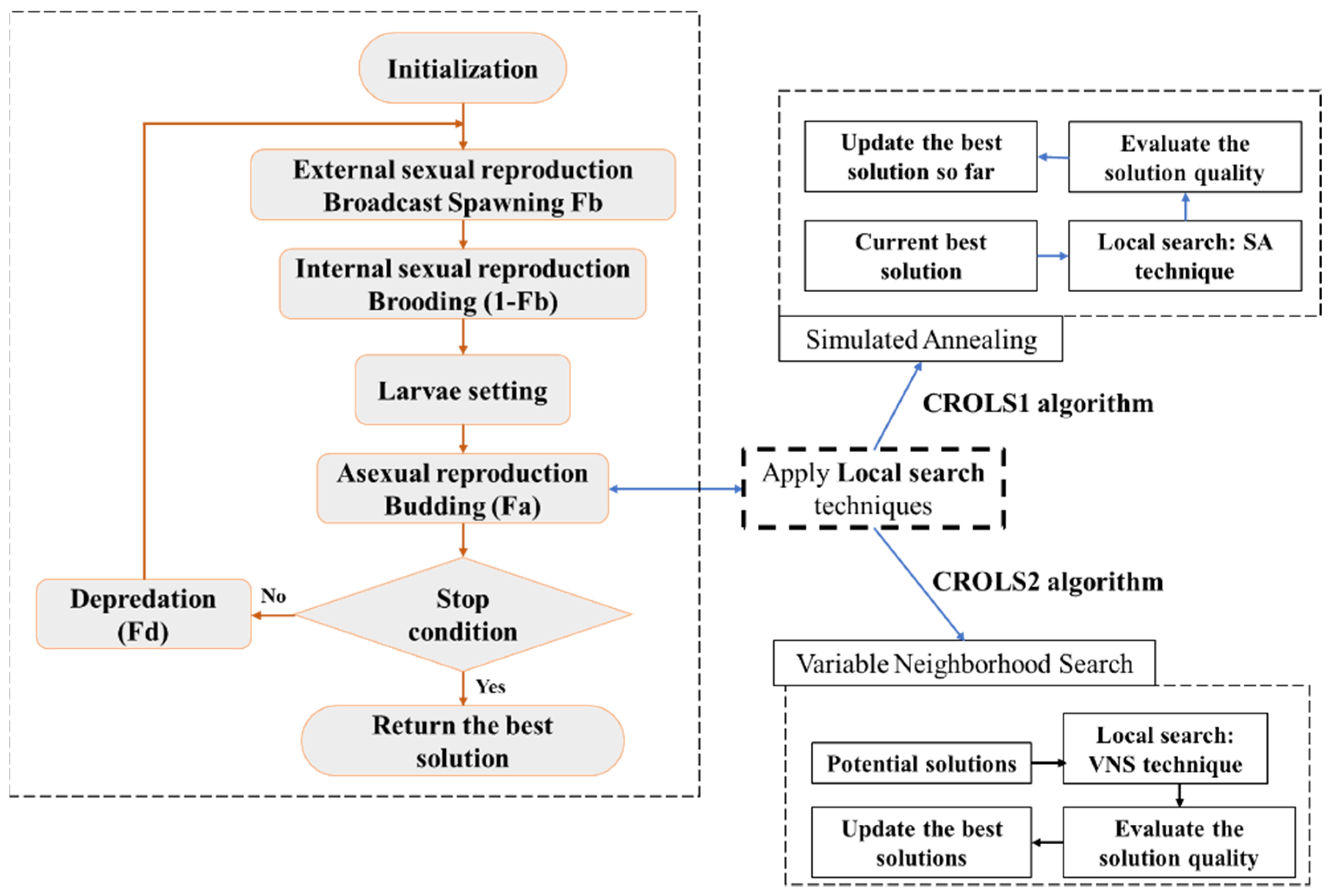
3.5. Proposal Approaches
| Algorithm 4: Hybrid Coral Reef Optimization Algorithms (CROLS1 and CROLS2) |
| Input: : reef size, : occupation rate, : fraction of broadcast spawners, : fraction of asexual reproduction, : fraction of the worse fitness corals, : the deprecated probability of the worse fitness corals. Output: Reasonable solution with best fitness #Initialization—Reef formation phase:
|
3.6. Time Complexity
4. Experiment Results and Discussion
4.1. Dataset
4.2. Parameters Used in the Algorithm
4.3. Experiment Results
4.3.1. Search Performance on CRO-Based Algorithm with Different Reef Sizes
4.3.2. Comparison of the Computational Result of CRO-Based Algorithms with Other Implemented Local Search Technique Algorithms
4.3.3. Comparison of the Computational Result of CRO-Based Algorithms with Other Contemporary Algorithms
4.3.4. Improvement of Search Efficiency
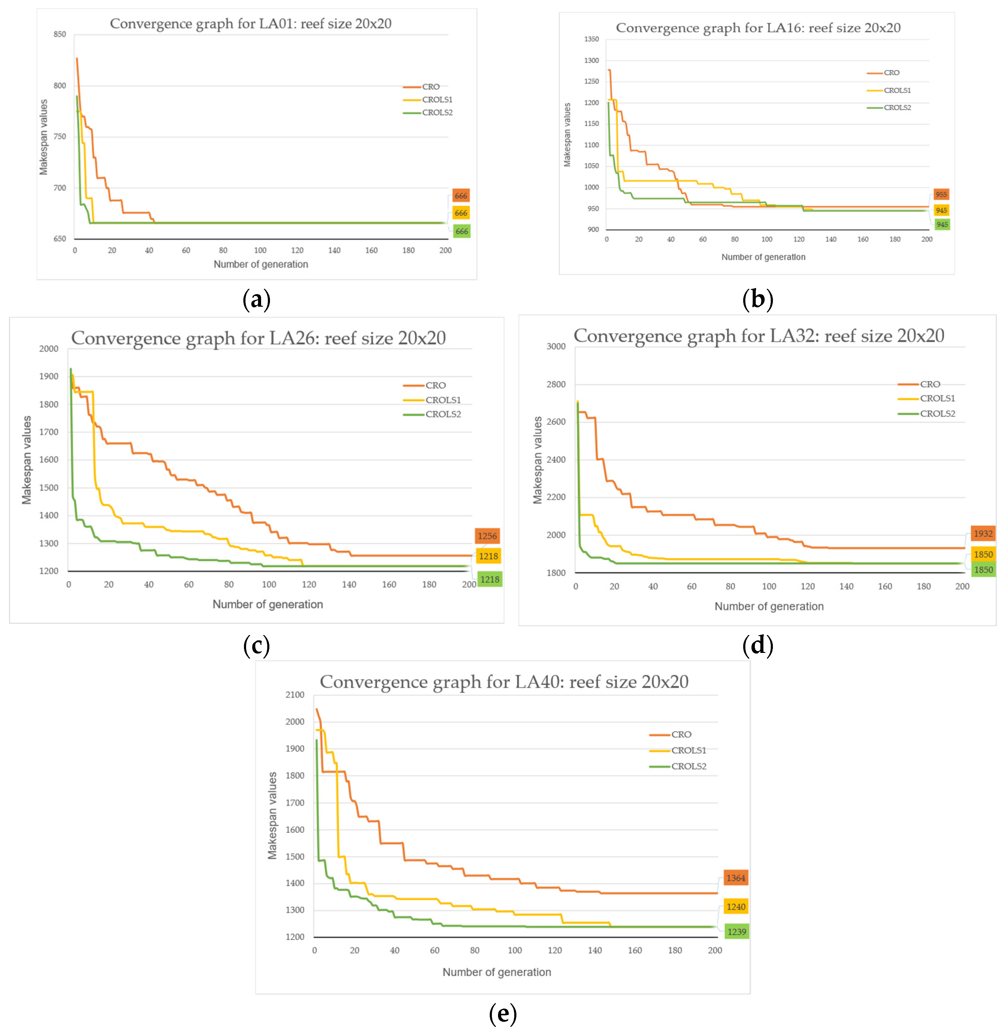
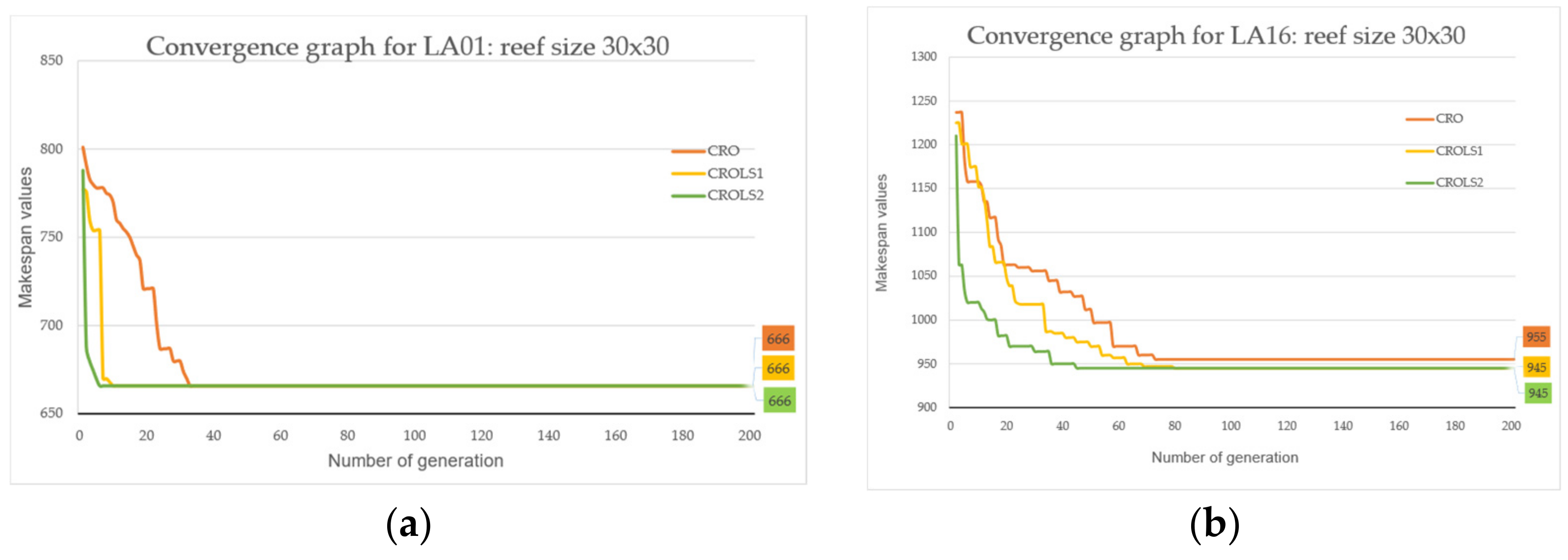
4.3.5. Convergence Ability
5. Conclusions
Author Contributions
Funding
Institutional Review Board Statement
Informed Consent Statement
Data Availability Statement
Acknowledgments
Conflicts of Interest
References
- Baptista, M. How Important Is Production Scheduling Today? April 2020. Available online: https://blogs.sw.siemens.com/opcenter/how-important-is-production-scheduling-today/ (accessed on 31 August 2022).
- Ben Hmida, J.; Lee, J.; Wang, X.; Boukadi, F. Production scheduling for continuous manufacturing systems with quality constraints. Prod. Manuf. Res. 2014, 2, 95–111. [Google Scholar] [CrossRef][Green Version]
- Jiang, Z.; Yuan, S.; Ma, J.; Wang, Q. The evolution of production scheduling from Industry 3.0 through Industry 4.0. Int. J. Prod. Res. 2021, 60, 3534–3554. [Google Scholar] [CrossRef]
- Graves, S.C. A Review of Production Scheduling. Oper. Res. 1981, 29, 646–675. [Google Scholar] [CrossRef]
- Johnson, S.M. Optimal two- and three-stage production schedules with setup times included. Nav. Res. Logist. Q. 1954, 1, 61–68. [Google Scholar] [CrossRef]
- Garey, M.R.; Johnson, D.S.; Sethi, R. The Complexity of Flowshop and Jobshop Scheduling. Math. Oper. Res. 1976, 1, 117–129. [Google Scholar] [CrossRef]
- Zhang, J.; Ding, G.; Zou, Y.; Qin, S.; Fu, J. Review of job shop scheduling research and its new perspectives under Industry 4.0. J. Intell. Manuf. 2017, 30, 1809–1830. [Google Scholar] [CrossRef]
- Xiong, H.; Shi, S.; Ren, D.; Hu, J. A survey of job shop scheduling problem: The types and models. Comput. Oper. Res. 2022, 142, 105731. [Google Scholar] [CrossRef]
- Xhafa, F.; Abraham, A. Metaheuristics for Scheduling in Industrial and Manufacturing Applications. Available online: https://link.springer.com/book/10.1007/978-3-540-78985-7 (accessed on 1 July 2022).
- Pinedo, M.L. Planning and Scheduling in Manufacturing and Services. 2009. Available online: https://link.springer.com/book/10.1007/978-1-4419-0910-7 (accessed on 3 July 2022).
- Türkyılmaz, A.; Şenvar, Ö.; Ünal, I.; Bulkan, S. A research survey: Heuristic approaches for solving multi objective flexible job shop problems. J. Intell. Manuf. 2020, 31, 1949–1983. [Google Scholar] [CrossRef]
- Guzman, E.; Andres, B.; Poler, R. Matheuristic Algorithm for Job-Shop Scheduling Problem Using a Disjunctive Mathematical Model. Computers 2021, 11, 1. [Google Scholar] [CrossRef]
- Viana, M.S.; Contreras, R.C.; Junior, O.M. A New Frequency Analysis Operator for Population Improvement in Genetic Algorithms to Solve the Job Shop Scheduling Problem. Sensors 2022, 22, 4561. [Google Scholar] [CrossRef]
- Salcedo-Sanz, S.; Del Ser, J.; Landa-Torres, I.; Gil-López, S.; Portilla-Figueras, J.A. The Coral Reefs Optimization Algorithm: A Novel Metaheuristic for Efficiently Solving Optimization Problems. Sci. World J. 2014, 2014, 739768. [Google Scholar] [CrossRef] [PubMed]
- Salcedo-Sanz, S.; García-Díaz, P.; Portilla-Figueras, J.; Del Ser, J.; Gil-López, S. A Coral Reefs Optimization algorithm for optimal mobile network deployment with electromagnetic pollution control criterion. Appl. Soft Comput. 2014, 24, 239–248. [Google Scholar] [CrossRef]
- Salcedo-Sanz, S.; Camacho-Gómez, C.; Mallol-Poyato, R.; Jiménez-Fernández, S.; Del Ser, J. A novel Coral Reefs Optimization algorithm with substrate layers for optimal battery scheduling optimization in micro-grids. Soft Comput. 2016, 20, 4287–4300. [Google Scholar] [CrossRef]
- Salcedo-Sanz, S.; Gallo-Marazuela, D.; Pastor-Sánchez, A.; Carro-Calvo, L.; Portilla-Figueras, A.; Prieto, L. Offshore wind farm design with the Coral Reefs Optimization algorithm. Renew. Energy 2014, 63, 109–115. [Google Scholar] [CrossRef]
- Bedoya-Valencia, L. Exact and Heuristic Algorithms for the Job Shop Scheduling Problem with Earliness and Tardiness over a Common Due Date. Ph.D. Thesis, Old Dominion University, Norfolk, VA, USA, 2007. [Google Scholar]
- Brucker, P.; Jurisch, B.; Sievers, B. A branch and bound algorithm for the job-shop scheduling problem. Discret. Appl. Math. 1994, 49, 107–127. [Google Scholar] [CrossRef]
- Çaliş, B.; Bulkan, S. A research survey: Review of AI solution strategies of job shop scheduling problem. J. Intell. Manuf. 2013, 26, 961–973. [Google Scholar] [CrossRef]
- Muthuraman, S.; Venkatesan, V.P. A Comprehensive Study on Hybrid Meta-Heuristic Approaches Used for Solving Combinatorial Optimization Problems. In Proceedings of the 2017 World Congress on Computing and Communication Technologies (WCCCT), Tiruchirappalli, India, 2–4 February 2017; pp. 185–190. [Google Scholar] [CrossRef]
- Aarts, E.; Aarts, E.H.; Lenstra, J.K. Local Search in Combinatorial Optimization. 2003. Available online: https://press.princeton.edu/books/paperback/9780691115221/local-search-in-combinatorial-optimization (accessed on 3 July 2022).
- Gendreau, M.; Potvin, J.-Y. Metaheuristics in Combinatorial Optimization. Ann. Oper. Res. 2005, 140, 189–213. [Google Scholar] [CrossRef]
- Yang, X.-S. (Ed.) Nature-Inspired Optimization Algorithms; Elsevier: Oxford, UK, 2014. [Google Scholar] [CrossRef]
- Davis, L. Job Shop Scheduling with Genetic Algorithms. In Proceedings of the 1st International Conference on Genetic Algorithms, Pittsburgh, PA, USA, 24–26 July 1985; pp. 136–140. [Google Scholar]
- Holland, J.H. Adaptation in Natural and Artificial Systems: An Introductory Analysis with Applications to Biology, Control, and Artificial Intelligence. MIT Press eBooks. IEEE Xplore. Available online: https://ieeexplore.ieee.org/book/6267401 (accessed on 3 July 2022).
- Kennedy, J.; Eberhart, R. Particle Swarm Optimization. In Proceedings of the ICNN’95—International Conference on Neural Networks, Perth, Australia, 27 November–1 December 1995; Volume 4, pp. 1942–1948. [Google Scholar] [CrossRef]
- Kirkpatrick, S.; Gelatt, C.D., Jr.; Vecchi, M.P. Optimization by Simulated Annealing. Science 1983, 220, 671–680. [Google Scholar] [CrossRef]
- Wang, S.-J.; Tsai, C.-W.; Chiang, M.-C. A High Performance Search Algorithm for Job-Shop Scheduling Problem. Procedia Comput. Sci. 2018, 141, 119–126. [Google Scholar] [CrossRef]
- Yu, H.; Gao, Y.; Wang, L.; Meng, J. A Hybrid Particle Swarm Optimization Algorithm Enhanced with Nonlinear Inertial Weight and Gaussian Mutation for Job Shop Scheduling Problems. Mathematics 2020, 8, 1355. [Google Scholar] [CrossRef]
- Kurdi, M. An effective genetic algorithm with a critical-path-guided Giffler and Thompson crossover operator for job shop scheduling problem. Int. J. Intell. Syst. Appl. Eng. 2019, 7, 13–18. [Google Scholar] [CrossRef][Green Version]
- Jiang, T.; Zhang, C. Application of Grey Wolf Optimization for Solving Combinatorial Problems: Job Shop and Flexible Job Shop Scheduling Cases. IEEE Access 2018, 6, 26231–26240. [Google Scholar] [CrossRef]
- Wang, F.; Tian, Y.; Wang, X. A Discrete Wolf Pack Algorithm for Job Shop Scheduling Problem. In Proceedings of the 2019 5th International Conference on Control, Automation and Robotics (ICCAR), Beijing, China, 19–22 April 2019; pp. 581–585. [Google Scholar] [CrossRef]
- Hamzadayı, A.; Baykasoğlu, A.; Akpınar, Ş. Solving combinatorial optimization problems with single seekers society algorithm. Knowl.-Based Syst. 2020, 201–202, 106036. [Google Scholar] [CrossRef]
- Garcia-Hernandez, L.; Salas-Morera, L.; Carmona-Munoz, C.; Abraham, A.; Salcedo-Sanz, S. A Hybrid Coral Reefs Optimization—Variable Neighborhood Search Approach for the Unequal Area Facility Layout Problem. IEEE Access 2020, 8, 134042–134050. [Google Scholar] [CrossRef]
- Tsai, C.-W.; Chang, H.-C.; Hu, K.-C.; Chiang, M.-C. Parallel coral reef algorithm for solving JSP on Spark. In Proceedings of the 2016 IEEE International Conference on Systems, Man, and Cybernetics (SMC), Budapest, Hungary, 9–12 October 2016; pp. 001872–001877. [Google Scholar] [CrossRef]
- Cheng, R.; Gen, M.; Tsujimura, Y. A tutorial survey of job-shop scheduling problems using genetic algorithms—I. Representation. Comput. Ind. Eng. 1996, 30, 983–997. [Google Scholar] [CrossRef]
- Cheng, R.; Gen, M.; Tsujimura, Y. A tutorial survey of job-shop scheduling problems using genetic algorithms, Part II: Hybrid genetic search strategies. Comput. Ind. Eng. 1999, 36, 343–364. [Google Scholar] [CrossRef]
- Lee, Y.S.; Graham, E.; Jackson, G.; Galindo, A.; Adjiman, C.S. A comparison of the performance of multi-objective optimization methodologies for solvent design. In Computer Aided Chemical Engineering; Kiss, A.A., Zondervan, E., Lakerveld, R., Özkan, L., Eds.; Elsevier: Amsterdam, The Netherlands, 2019; Volume 46, pp. 37–42. [Google Scholar] [CrossRef]
- Ruiz, J.; Garcia, G. Simulated Annealing Evolution; IntechOpen: London, UK, 2012. [Google Scholar] [CrossRef]
- Mladenović, N.; Hansen, P. Variable neighborhood search. Comput. Oper. Res. 1997, 24, 1097–1100. [Google Scholar] [CrossRef]
- Hansen, P.; Mladenović, N.; Urošević, D. Variable neighborhood search for the maximum clique. Discret. Appl. Math. 2004, 145, 117–125. [Google Scholar] [CrossRef]
- Lawrence, S. Resource constrained project scheduling: An experimental investigation of heuristic scheduling techniques (Supplement). Master’s Thesis, Graduate School of Industrial Administration, Pittsburgh, PA, USA, 1984. [Google Scholar]
- Qing-Dao-Er-Ji, R.; Wang, Y. A new hybrid genetic algorithm for job shop scheduling problem. Comput. Oper. Res. 2012, 39, 2291–2299. [Google Scholar] [CrossRef]
- Gao, L.; Zhang, G.; Zhang, L.; Li, X. An efficient memetic algorithm for solving the job shop scheduling problem. Comput. Ind. Eng. 2011, 60, 699–705. [Google Scholar] [CrossRef]
- Fisher, C.; Thompson, G. Probabilistic Learning Combinations of Local Job-shop Scheduling Rules; Industrial Scheduling: Englewood Cliffs, NJ, USA, 1963; pp. 225–251. [Google Scholar]
- Applegate, D.; Cook, W. A Computational Study of the Job-Shop Scheduling Problem. Informs J. Comput. 1991, 3, 149–156. [Google Scholar] [CrossRef]
- Adams, J.; Balas, E.; Zawack, D. The Shifting Bottleneck Procedure for Job Shop Scheduling. Manag. Sci. 1988, 34, 391–401. [Google Scholar] [CrossRef]
- Viana, M.S.; Junior, O.M.; Contreras, R.C. An Improved Local Search Genetic Algorithm with Multi-crossover for Job Shop Scheduling Problem. In Artificial Intelligence and Soft Computing; Springer: Cham, Swizerland, 2020; pp. 464–479. [Google Scholar] [CrossRef]


| Parameter | Technique | Definition | Range |
|---|---|---|---|
| CRO | Reef size | ] | |
| Iter | CRO | Number of iterations (generations) | |
| Fb | CRO | Probability of Broadcast spawning process | |
| Fa | CRO | Probability of Budding process | |
| r0 | CRO | Initial free/occupied ratio | |
| Fd | CRO | Probability of selecting weak individuals from the population | |
| Pd | CRO | Probability of removing weak individuals from the population | |
| k | CRO | Number of chances for a new coral to colonize a reef | |
| ke | CRO | Maximum number of allowed equal corals | |
| SA | Min temperature | [0.0001, 1] | |
| SA | Cooling rate | [0.7, 0.99] | |
| VNS | Solution set in neighborhood structure | [1, L] |
| Size | r0 | Fb | Fa | Fd | Pd | k | tmin | α | Nk | |
|---|---|---|---|---|---|---|---|---|---|---|
| Small | 0.6 | 0.9 | 0.05 | 0.01 | 0.1 | 3 | 0.5 | 0.85 | L | |
| Medium | 0.7 | 0.85 | 0.05 | 0.05 | 0.1 | 3 | 0.5 | 0.85 | L | |
| Large | 0.7 | 0.85 | 0.1 | 0.1 | 0.1 | 3 | 0.5 | 0.85 | L |
| Instance | Size | Reef Size | Method | Opt | Best | Worst | Mean | SD | Time (s) |
|---|---|---|---|---|---|---|---|---|---|
| LA01 | 10 × 10 | CRO | 666 | 666 | 674 | 668.91 | 2.4 | 128.45 | |
| CROLS1 | 666 | 666 | 666 | 666 | 0 | 39.91 | |||
| CROLS2 | 666 | 666 | 666 | 666 | 0 | 33.18 | |||
| 20 × 20 | CRO | 666 | 666 | 671 | 667.73 | 1.58 | 45.09 | ||
| CROLS1 | 666 | 666 | 671 | 668.45 | 1.79 | 20.45 | |||
| CROLS2 | 666 | 666 | 666 | 666 | 0 | 15.64 | |||
| 30 × 30 | CRO | 666 | 666 | 674 | 669.55 | 2.7 | 44.27 | ||
| CROLS1 | 666 | 666 | 671 | 668.09 | 2 | 20.27 | |||
| CROLS2 | 666 | 666 | 671 | 667.45 | 1.91 | 14.64 | |||
| LA02 | 10 × 10 | CRO | 655 | 655 | 676 | 664.91 | 6.41 | 118.73 | |
| CROLS1 | 655 | 655 | 655 | 655 | 0 | 40.91 | |||
| CROLS2 | 655 | 655 | 655 | 655 | 0 | 33.91 | |||
| 20 × 20 | CRO | 655 | 655 | 671 | 663.73 | 5.68 | 43.82 | ||
| CROLS1 | 655 | 655 | 671 | 662.27 | 5.57 | 18.55 | |||
| CROLS2 | 655 | 655 | 655 | 655 | 0 | 15.27 | |||
| 30 × 30 | CRO | 655 | 655 | 676 | 665.36 | 6.62 | 44.55 | ||
| CROLS1 | 655 | 655 | 671 | 663.18 | 6.02 | 18.55 | |||
| CROLS2 | 655 | 655 | 670 | 661.09 | 6.21 | 14.09 | |||
| LA06 | 10 × 10 | CRO | 926 | 926 | 946 | 935.45 | 7.54 | 169.09 | |
| CROLS1 | 926 | 926 | 926 | 926 | 0 | 151.82 | |||
| CROLS2 | 926 | 926 | 926 | 926 | 0 | 149.73 | |||
| 20 × 20 | CRO | 926 | 926 | 940 | 931.73 | 4.73 | 125.91 | ||
| CROLS1 | 926 | 926 | 940 | 932.36 | 5.46 | 100.73 | |||
| CROLS2 | 926 | 926 | 926 | 926 | 0 | 92.45 | |||
| 30 × 30 | CRO | 926 | 926 | 946 | 935 | 7.82 | 76.36 | ||
| CROLS1 | 926 | 926 | 940 | 931.18 | 5.04 | 46.55 | |||
| CROLS2 | 926 | 926 | 940 | 933.18 | 5.09 | 41.09 | |||
| LA07 | 10 × 10 | CRO | 890 | 899 | 922 | 906.45 | 6.24 | 175.73 | |
| CROLS1 | 890 | 890 | 895 | 890.73 | 1.54 | 148.18 | |||
| CROLS2 | 890 | 890 | 892 | 890.45 | 0.81 | 133.55 | |||
| 20 × 20 | CRO | 890 | 895 | 916 | 905.73 | 5.8 | 117.91 | ||
| CROLS1 | 890 | 890 | 916 | 907 | 5.04 | 94.82 | |||
| CROLS2 | 890 | 890 | 890 | 890 | 0 | 88.73 | |||
| 30 × 30 | CRO | 890 | 890 | 922 | 908.18 | 7.38 | 78.09 | ||
| CROLS1 | 890 | 890 | 916 | 906.91 | 5.29 | 45.91 | |||
| CROLS2 | 890 | 890 | 916 | 905.09 | 5.92 | 33.64 | |||
| LA11 | 10 × 10 | CRO | 1222 | 1222 | 1257 | 1235.64 | 13.41 | 237.36 | |
| CROLS1 | 1222 | 1222 | 1222 | 1222 | 0 | 224.09 | |||
| CROLS2 | 1222 | 1222 | 1222 | 1222 | 0 | 229.73 | |||
| 20 × 20 | CRO | 1222 | 1222 | 1244 | 1228.55 | 7.15 | 166.91 | ||
| CROLS1 | 1222 | 1222 | 1244 | 1229.64 | 7.13 | 147.91 | |||
| CROLS2 | 1222 | 1222 | 1222 | 1222 | 0 | 136.55 | |||
| 30 × 30 | CRO | 1222 | 1222 | 1257 | 1233.45 | 12.58 | 128.82 | ||
| CROLS1 | 1222 | 1222 | 1244 | 1230.73 | 8.52 | 100.18 | |||
| CROLS2 | 1222 | 1222 | 1244 | 1229.91 | 7.89 | 95.72 | |||
| LA12 | 10 × 10 | CRO | 1039 | 1039 | 1062 | 1049.55 | 6.96 | 241.45 | |
| CROLS1 | 1039 | 1039 | 1042 | 1039.36 | 0.92 | 228.55 | |||
| CROLS2 | 1039 | 1039 | 1039 | 1039 | 0 | 217.64 | |||
| 20 × 20 | CRO | 1039 | 1039 | 1062 | 1049.55 | 6.87 | 164.27 | ||
| CROLS1 | 1039 | 1039 | 1062 | 1051.91 | 6.62 | 157.91 | |||
| CROLS2 | 1039 | 1039 | 1039 | 1039 | 0 | 149.91 | |||
| 30 × 30 | CRO | 1039 | 1039 | 1060 | 1048.27 | 7.96 | 120.09 | ||
| CROLS1 | 1039 | 1039 | 1043 | 1047.45 | 7.27 | 103.45 | |||
| CROLS2 | 1039 | 1039 | 1039 | 1050.91 | 7.01 | 89.91 | |||
| LA16 | 10 × 10 | CRO | 945 | 971 | 1024 | 979.27 | 22.73 | 349.64 | |
| CROLS1 | 945 | 945 | 979 | 958.91 | 10.69 | 317.73 | |||
| CROLS2 | 945 | 945 | 980 | 959.36 | 12.44 | 315.64 | |||
| 20 × 20 | CRO | 945 | 948 | 1011 | 981.91 | 17.11 | 239.73 | ||
| CROLS1 | 945 | 945 | 956 | 949.64 | 4.37 | 212.55 | |||
| CROLS2 | 945 | 945 | 955 | 948.91 | 4 | 198.64 | |||
| 30 × 30 | CRO | 945 | 948 | 1011 | 976.55 | 19.06 | 177.64 | ||
| CROLS1 | 945 | 945 | 955 | 947.73 | 2.93 | 125.91 | |||
| CROLS2 | 945 | 945 | 955 | 948.73 | 4.13 | 132.55 | |||
| LA17 | 10 × 10 | CRO | 784 | 799 | 888 | 833.55 | 31.06 | 337.09 | |
| CROLS1 | 784 | 787 | 807 | 795.18 | 7.55 | 309.73 | |||
| CROLS2 | 784 | 788 | 807 | 797.91 | 7.79 | 297.55 | |||
| 20 × 20 | CRO | 784 | 788 | 832 | 811.91 | 13.08 | 252.64 | ||
| CROLS1 | 784 | 784 | 788 | 785.36 | 1.69 | 198.55 | |||
| CROLS2 | 784 | 784 | 799 | 790.36 | 5.71 | 222.91 | |||
| 30 × 30 | CRO | 784 | 788 | 832 | 808.27 | 13.51 | 183.18 | ||
| CROLS1 | 784 | 784 | 799 | 788.55 | 4.88 | 128.82 | |||
| CROLS2 | 784 | 784 | 799 | 787.09 | 4.43 | 130.09 | |||
| LA21 | 10 × 10 | CRO | 1046 | 1069 | 1146 | 1105.73 | 79.28 | 553.64 | |
| CROLS1 | 1046 | 1056 | 1117 | 1100.64 | 10.07 | 487.18 | |||
| CROLS2 | 1046 | 1055 | 1115 | 1099 | 8.29 | 473.09 | |||
| 20 × 20 | CRO | 1046 | 1069 | 1100 | 1071.45 | 49.41 | 345.91 | ||
| CROLS1 | 1046 | 1046 | 1054 | 1048.82 | 3.27 | 269.36 | |||
| CROLS2 | 1046 | 1046 | 1066 | 1053.09 | 6.34 | 274.27 | |||
| 30 × 30 | CRO | 1046 | 1106 | 1250 | 1172.64 | 51.47 | 256.64 | ||
| CROLS1 | 1046 | 1046 | 1066 | 1052.55 | 7.76 | 164.36 | |||
| CROLS2 | 1046 | 1046 | 1066 | 1052.55 | 6.88 | 165.55 | |||
| LA22 | 10 × 10 | CRO | 927 | 978 | 1220 | 1178.36 | 30.51 | 538.45 | |
| CROLS1 | 927 | 930 | 1011 | 983.45 | 16.83 | 479.73 | |||
| CROLS2 | 927 | 934 | 988 | 976.09 | 8.32 | 464.09 | |||
| 20 × 20 | CRO | 927 | 944 | 1150 | 1030.64 | 57.45 | 356.27 | ||
| CROLS1 | 927 | 927 | 974 | 944.18 | 16.83 | 267.91 | |||
| CROLS2 | 927 | 927 | 944 | 932.18 | 4.8 | 265.55 | |||
| 30 × 30 | CRO | 927 | 935 | 1150 | 1030.09 | 53.54 | 248.27 | ||
| CROLS1 | 927 | 927 | 944 | 932.73 | 5.69 | 185.18 | |||
| CROLS2 | 927 | 927 | 944 | 934.27 | 6.21 | 174.27 | |||
| LA26 | 10 × 10 | CRO | 1218 | 1333 | 1358 | 1349.64 | 22.89 | 759.64 | |
| CROLS1 | 1218 | 1246 | 1316 | 1297.09 | 10.72 | 655.82 | |||
| CROLS2 | 1218 | 1242 | 1323 | 1305.82 | 12.36 | 651.91 | |||
| 20 × 20 | CRO | 1218 | 1256 | 1280 | 1263.27 | 45.98 | 536.64 | ||
| CROLS1 | 1218 | 1218 | 1253 | 1235.91 | 12.07 | 456.91 | |||
| CROLS2 | 1218 | 1218 | 1246 | 1230.27 | 8.97 | 440.36 | |||
| 30 × 30 | CRO | 1218 | 1226 | 1275 | 1255.82 | 44.37 | 359.91 | ||
| CROLS1 | 1218 | 1218 | 1246 | 1229.91 | 10.75 | 281.73 | |||
| CROLS2 | 1218 | 1218 | 1246 | 1231.09 | 9.12 | 246.27 | |||
| LA27 | 10 × 10 | CRO | 1235 | 1323 | 1495 | 1446.55 | 30.3 | 748.09 | |
| CROLS1 | 1235 | 1255 | 1310 | 1275.36 | 8.51 | 688.91 | |||
| CROLS2 | 1235 | 1256 | 1304 | 1261.09 | 8.29 | 650.64 | |||
| 20 × 20 | CRO | 1235 | 1305 | 1415 | 1461.09 | 22.57 | 541.09 | ||
| CROLS1 | 1235 | 1235 | 1305 | 1260.55 | 28.95 | 459.45 | |||
| CROLS2 | 1235 | 1235 | 1246 | 1239.18 | 4.1 | 447.36 | |||
| 30 × 30 | CRO | 1235 | 1255 | 1375 | 1359.55 | 25.96 | 336.18 | ||
| CROLS1 | 1235 | 1235 | 1246 | 1239.09 | 4.2 | 260.18 | |||
| CROLS2 | 1235 | 1235 | 1246 | 1240.27 | 4.09 | 239.27 | |||
| LA32 | 10 × 10 | CRO | 1850 | 1934 | 2328 | 2254.91 | 96.2 | 827.91 | |
| CROLS1 | 1850 | 1852 | 1896 | 1862.73 | 13.75 | 713.55 | |||
| CROLS2 | 1850 | 1850 | 1888 | 1866.73 | 9.77 | 693.09 | |||
| 20 × 20 | CRO | 1850 | 1932 | 2126 | 2074.85 | 30.69 | 740.73 | ||
| CROLS1 | 1850 | 1850 | 1865 | 1855.36 | 5.77 | 646.64 | |||
| CROLS2 | 1850 | 1850 | 1856 | 1852.18 | 2.29 | 630.18 | |||
| 30 × 30 | CRO | 1850 | 1912 | 2105 | 1998.52 | 30.26 | 566.64 | ||
| CROLS1 | 1850 | 1850 | 1856 | 1853 | 2.05 | 453.45 | |||
| CROLS2 | 1850 | 1850 | 1856 | 1852.18 | 2.33 | 418.45 | |||
| LA33 | 10 × 10 | CRO | 1719 | 1865 | 2131 | 2014.73 | 65 | 824.18 | |
| CROLS1 | 1719 | 1720 | 1752 | 1732.27 | 12.43 | 726.09 | |||
| CROLS2 | 1719 | 1722 | 1752 | 1730.27 | 11.39 | 692.82 | |||
| 20 × 20 | CRO | 1719 | 1818 | 2056 | 1955.73 | 55.54 | 737.91 | ||
| CROLS1 | 1719 | 1719 | 1723 | 1720.45 | 1.56 | 643.09 | |||
| CROLS2 | 1719 | 1719 | 1732 | 1723.91 | 5.48 | 617.27 | |||
| 30 × 30 | CRO | 1719 | 1805 | 2034 | 1934.91 | 60.59 | 557.82 | ||
| CROLS1 | 1719 | 1719 | 1732 | 1723.45 | 4.97 | 441.73 | |||
| CROLS2 | 1719 | 1719 | 1732 | 1724.18 | 5.14 | 438.82 | |||
| LA39 | 10 × 10 | CRO | 1233 | 1388 | 1466 | 1498.82 | 42.44 | 869.09 | |
| CROLS1 | 1233 | 1238 | 1316 | 1278.73 | 16.66 | 725.73 | |||
| CROLS2 | 1233 | 1274 | 1318 | 1279.82 | 13.48 | 624.45 | |||
| 20 × 20 | CRO | 1233 | 1368 | 1428 | 1419.36 | 7.61 | 834.09 | ||
| CROLS1 | 1233 | 1238 | 1264 | 1241.64 | 27.32 | 675.45 | |||
| CROLS2 | 1233 | 1239 | 1264 | 1244.91 | 29.39 | 568.73 | |||
| 30 × 30 | CRO | 1233 | 1332 | 1403 | 1397.21 | 24.37 | 752.09 | ||
| CROLS1 | 1233 | 1233 | 1255 | 1243.09 | 34.44 | 592.64 | |||
| CROLS2 | 1233 | 1233 | 1255 | 1237.55 | 13.78 | 502.82 | |||
| LA40 | 10 × 10 | CRO | 1222 | 1396 | 1506 | 1451.25 | 49.25 | 875 | |
| CROLS1 | 1222 | 1240 | 1336 | 1313.27 | 11.24 | 728.45 | |||
| CROLS2 | 1222 | 1269 | 1305 | 1288.45 | 35.41 | 625.36 | |||
| 20 × 20 | CRO | 1222 | 1364 | 1455 | 1390.35 | 58.7 | 826.82 | ||
| CROLS1 | 1222 | 1240 | 1299 | 1270.27 | 35.09 | 674.73 | |||
| CROLS2 | 1222 | 1239 | 1299 | 1273.09 | 30.93 | 568.82 | |||
| 30 × 30 | CRO | 1222 | 1342 | 1424 | 1374.33 | 24.88 | 739.82 | ||
| CROLS1 | 1222 | 1228 | 1264 | 1238.25 | 15.89 | 585.45 | |||
| CROLS2 | 1222 | 1232 | 1279 | 1248.45 | 23.22 | 495.55 |
| Algorithm | Mean Rank | ||
|---|---|---|---|
| Reef Size 10 × 10 | Reef Size 20 × 20 | Reef Size 30 × 30 | |
| CRO | 3.00 | 2.69 | 2.94 |
| CROLS1 | 1.56 | 2.06 | 1.47 |
| CROLS2 | 1.44 | 1.25 | 1.59 |
| Χ2 | ρ | |
|---|---|---|
| Reef Size 10 × 10 | 25.733 | 0.000003 |
| Reef Size 20 × 20 | 16.625 | 0.000245 |
| Reef Size 30 × 30 | 21.556 | 0.000021 |
| CRO-CROLS1 | CRO-CROLS2 | CROLS1-CROLS2 | |
|---|---|---|---|
| Z | −3.516 | −3.516 | −1.533 |
| p | 0.000438 | 0.000438 | 0.125153 |
| Ins. | Size. | Opt. | CRO | CROLS1 | CROLS2 | HGA | MA | ||||||
|---|---|---|---|---|---|---|---|---|---|---|---|---|---|
| 10 × 10 | 20 × 20 | 30 × 30 | 10 × 10 | 20 × 20 | 30 × 30 | 10 × 10 | 20 × 20 | 30 × 30 | |||||
| LA01 | 666 | 666 | 666 | 666 | 666 | 666 | 666 | 666 | 666 | 666 | 666 | 666 | |
| LA02 | 655 | 655 | 655 | 655 | 655 | 655 | 655 | 655 | 655 | 655 | 655 | 655 | |
| LA06 | 926 | 926 | 926 | 926 | 926 | 926 | 926 | 926 | 926 | 926 | 926 | 926 | |
| LA07 | 890 | 899 | 895 | 890 | 890 | 890 | 890 | 890 | 890 | 890 | 890 | 890 | |
| LA11 | 1222 | 1228 | 1222 | 1222 | 1222 | 1222 | 1222 | 1222 | 1222 | 1222 | 1222 | 1222 | |
| LA12 | 1039 | 1042 | 1039 | 1039 | 1039 | 1039 | 1039 | 1039 | 1039 | 1039 | 1039 | 1039 | |
| LA16 | 945 | 956 | 955 | 955 | 945 | 945 | 945 | 945 | 945 | 945 | 945 | 945 | |
| LA17 | 784 | 799 | 788 | 788 | 787 | 784 | 784 | 788 | 784 | 784 | 784 | 784 | |
| LA21 | 1046 | 1069 | 1069.9 | 1056 | 1046 | 1046 | 1046 | 1055 | 1046 | 1046 | 1046 | 1055 | |
| LA22 | 927 | 978 | 944 | 935 | 930 | 927 | 927 | 934 | 928 | 927 | 935 | 927 | |
| LA26 | 1218 | 1333 | 1256 | 1226 | 1246 | 1218 | 1218 | 1242 | 1218 | 1218 | 1218 | 1218 | |
| LA27 | 1235 | 1323 | 1305 | 1255 | 1255 | 1235 | 1235 | 1256 | 1246 | 1246 | 1236 | 1261 | |
| LA32 | 1850 | 1934 | 1932 | 1912 | 1852 | 1850 | 1850 | 1850 | 1850 | 1850 | 1850 | 1850 | |
| LA33 | 1719 | 1865 | 1818 | 1805 | 1720 | 1719 | 1719 | 1722 | 1719 | 1719 | 1719 | 1719 | |
| LA39 | 1233 | 1388 | 1368 | 1332 | 1238 | 1238 | 1233 | 1274 | 1239 | 1233 | 1233 | 1241 | |
| LA40 | 1222 | 1396 | 1364 | 1342 | 1240 | 1240 | 1228 | 1269 | 1239 | 1232 | 1229 | 1233 | |
| Instance | Size | BKS | CRO | CROLS1 | CROLS2 | mXLSGA (2020) | NGPSO (2020) | SSS (2020) | GA-CPG-GT (2019) | DWPA (2019) |
|---|---|---|---|---|---|---|---|---|---|---|
| LA01 | 10 × 5 | 666 | 666 | 666 | 666 | 666 | 666 | 666 | 666 | 666 |
| LA02 | 10 × 5 | 655 | 655 | 655 | 655 | 655 | 655 | 655 | 655 | 655 |
| LA06 | 15 × 5 | 926 | 926 | 926 | 926 | 926 | 926 | 926 | 926 | 926 |
| LA07 | 15 × 5 | 890 | 890 | 890 | 890 | 890 | 890 | 890 | 890 | 890 |
| LA11 | 20 × 5 | 1222 | 1222 | 1222 | 1222 | 1222 | 1222 | 1222 | 1222 | 1222 |
| LA12 | 20 × 5 | 1039 | 1039 | 1039 | 1039 | 1039 | 1039 | - | 1039 | 1039 |
| LA16 | 10 × 10 | 945 | 955 | 945 | 945 | 945 | 945 | 947 | 946 | 993 |
| LA17 | 10 × 10 | 784 | 788 | 784 | 784 | 784 | 794 | - | 784 | 793 |
| LA21 | 15 × 10 | 1046 | 1056 | 1046 | 1046 | 1059 | 1183 | 1076 | 1090 | 1105 |
| LA22 | 15 × 10 | 927 | 935 | 927 | 927 | 935 | 927 | - | 954 | 989 |
| LA26 | 20 × 10 | 1218 | 1226 | 1218 | 1218 | 1218 | 1218 | - | 1237 | 1303 |
| LA27 | 20 × 10 | 1235 | 1255 | 1235 | 1246 | 1269 | 1394 | - | 1313 | 1346 |
| LA32 | 30 × 10 | 1850 | 1912 | 1850 | 1850 | 1850 | 1850 | - | 1850 | 1850 |
| LA33 | 30 × 10 | 1719 | 1805 | 1719 | 1719 | 1719 | 1719 | - | 1719 | 1719 |
| LA39 | 15 × 15 | 1233 | 1332 | 1233 | 1233 | 1258 | 1662 | - | 1290 | 1334 |
| LA40 | 15 × 15 | 1222 | 1342 | 1228 | 1232 | 1243 | 1222 | 1252 | 1252 | 1347 |
| FT06 | 6 × 6 | 55 | 55 | 55 | 55 | 55 | 55 | 55 | 55 | - |
| FT10 | 10 × 10 | 930 | 934 | 930 | 930 | 930 | 930 | 936 | 935 | - |
| FT20 | 20 × 5 | 1165 | 1197 | 1174 | 1170 | 1165 | 1210 | 1165 | 1180 | - |
| ABZ05 | 10 × 10 | 1234 | 1255 | 1234 | 1234 | 1234 | 1234 | - | 1238 | - |
| ABZ06 | 10 × 10 | 943 | 988 | 943 | 943 | 943 | 943 | - | 947 | - |
| ABZ07 | 20 × 15 | 656 | 755 | 731 | 727 | 695 | 713 | - | - | - |
| ABZ08 | 20 × 15 | 665 | 720 | 709 | 705 | 713 | 729 | - | - | - |
| ABZ09 | 20 × 15 | 679 | 817 | 707 | 711 | 721 | 930 | - | - | - |
| ORB01 | 10 × 10 | 1059 | 1120 | 1070 | 1072 | 1068 | 1174 | - | 1084 | - |
| ORB02 | 10 × 10 | 888 | 927 | 899 | 895 | 889 | 913 | - | 890 | - |
| ORB03 | 10 × 10 | 1005 | 1097 | 1021 | 1023 | 1023 | 1104 | - | 1037 | - |
| ORB04 | 10 × 10 | 1005 | 1121 | 1005 | 1005 | 1005 | 1005 | - | 1028 | - |
| ORB05 | 10 × 10 | 887 | 904 | 890 | 894 | 889 | 887 | - | 894 | - |
| ORB06 | 10 × 10 | 1010 | 1085 | 1020 | 1023 | 1019 | 1124 | - | 1035 | - |
| ORB07 | 10 × 10 | 397 | 418 | 397 | 397 | 397 | 397 | - | 404 | - |
| ORB08 | 10 × 10 | 899 | 988 | 912 | 907 | 907 | 1020 | - | 937 | - |
| ORB09 | 10 × 10 | 934 | 955 | 938 | 940 | 940 | 980 | - | 943 | - |
| ORB10 | 10 × 10 | 944 | 1010 | 967 | 950 | 944 | 1027 | - | 967 | - |
| Instance | Size | CROLS1 | CROLS2 | ||||
|---|---|---|---|---|---|---|---|
| 10 × 10 | 20 × 20 | 30 × 30 | 10 × 10 | 20 × 20 | 30 × 30 | ||
| LA01 | 0 | 0 | 0 | 0 | 0 | 0 | |
| LA02 | 1.68 | 0.46 | 0.15 | 1.68 | 0.46 | 0.15 | |
| LA06 | 0 | 0 | 0 | 0 | 0 | 0 | |
| LA07 | 1.01 | 0.56 | 0 | 1.01 | 0.56 | 0 | |
| LA11 | 0.49 | 0 | 0 | 0.49 | 0 | 0 | |
| LA12 | 0.29 | 0 | 0 | 0.29 | 0 | 0 | |
| LA16 | 2.43 | 0.32 | 0.32 | 2.75 | 0.32 | 0.32 | |
| LA17 | 1.53 | 0.51 | 0.51 | 1.4 | 0.51 | 0.51 | |
| LA21 | 2.2 | 2.28 | 0.96 | 1.34 | 2.28 | 0.96 | |
| LA22 | 5.18 | 1.83 | 0.86 | 4.75 | 1.73 | 0.86 | |
| LA26 | 7.14 | 3.12 | 0.66 | 7.47 | 3.12 | 0.66 | |
| LA27 | 5.51 | 5.67 | 1.62 | 5.43 | 4.78 | 0.73 | |
| LA32 | 4.43 | 4.43 | 3.35 | 4.54 | 4.43 | 3.35 | |
| LA33 | 8.44 | 5.76 | 5 | 8.32 | 5.76 | 5 | |
| LA39 | 12.17 | 10.54 | 8.03 | 9.25 | 10.46 | 8.03 | |
| LA40 | 12.77 | 10.15 | 9.33 | 10.39 | 10.23 | 9 | |
| Reef Size | 10 × 10 | 20 × 20 | 30 × 30 |
|---|---|---|---|
| CRO | 150.5 | 42.2 | 30.4 |
| CROLS1 | 13.4 | 10.6 | 10.4 |
| CROLS2 | 12.2 | 8 | 6.4 |
Publisher’s Note: MDPI stays neutral with regard to jurisdictional claims in published maps and institutional affiliations. |
© 2022 by the authors. Licensee MDPI, Basel, Switzerland. This article is an open access article distributed under the terms and conditions of the Creative Commons Attribution (CC BY) license (https://creativecommons.org/licenses/by/4.0/).
Share and Cite
Shieh, C.-S.; Nguyen, T.-T.; Lin, W.-W.; Nguyen, D.-C.; Horng, M.-F. Modified Coral Reef Optimization Methods for Job Shop Scheduling Problems. Appl. Sci. 2022, 12, 9867. https://doi.org/10.3390/app12199867
Shieh C-S, Nguyen T-T, Lin W-W, Nguyen D-C, Horng M-F. Modified Coral Reef Optimization Methods for Job Shop Scheduling Problems. Applied Sciences. 2022; 12(19):9867. https://doi.org/10.3390/app12199867
Chicago/Turabian StyleShieh, Chin-Shiuh, Thanh-Tuan Nguyen, Wan-Wei Lin, Dinh-Cuong Nguyen, and Mong-Fong Horng. 2022. "Modified Coral Reef Optimization Methods for Job Shop Scheduling Problems" Applied Sciences 12, no. 19: 9867. https://doi.org/10.3390/app12199867
APA StyleShieh, C.-S., Nguyen, T.-T., Lin, W.-W., Nguyen, D.-C., & Horng, M.-F. (2022). Modified Coral Reef Optimization Methods for Job Shop Scheduling Problems. Applied Sciences, 12(19), 9867. https://doi.org/10.3390/app12199867