

Path Planning for Multi-Arm Manipulators Using Soft Actor-Critic Algorithm with Position Prediction of Moving Obstacles via LSTM


Abstract
1. Introduction
1.1. Background and Motivation
1.2. Related Work
1.3. Proposed Method
2. Background Concept and Problem Modeling
2.1. Path Planning for Robot Manipulator and Configuration Space
2.2. Collision Detection in Workspace Using the Oriented Bounding Box (OBB)
2.3. Reinforcement Learning
2.4. Long Short-Term Memory (LSTM)
3. Soft Actor-Critic Based Path Planning for Moving Obstacles with LSTM
3.1. Path Planning for the Multi-Arm Manipulator and Augmented Configuration Space
3.2. Multi-Arm Manipulator MDP with Position Estimation of Moving Obstacles via LSTM
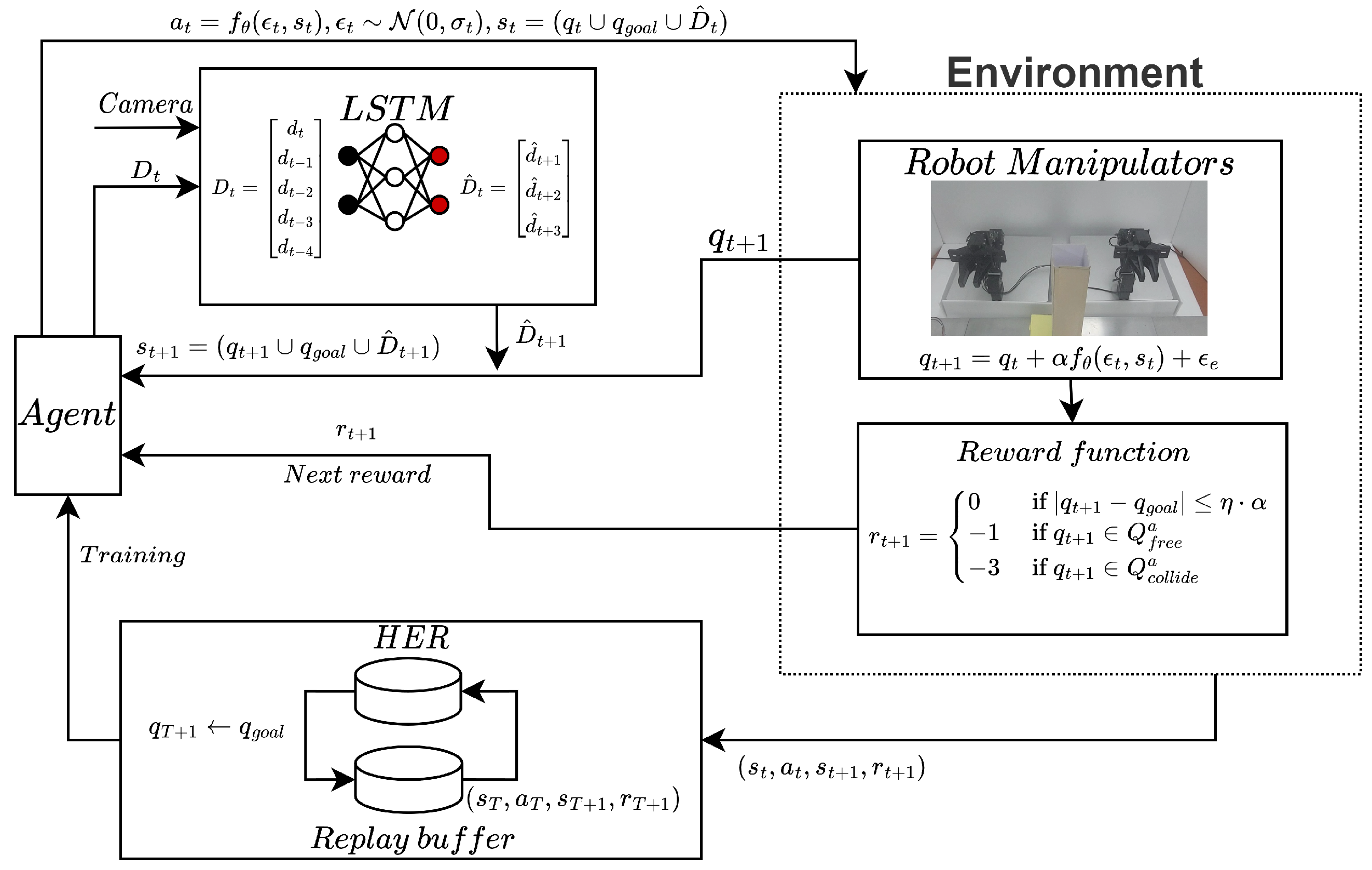
3.3. Soft Actor-Critic (SAC)-Based Path Planning with Prediction of Moving Obstacle Position via LSTM
| Algorithm 1 Proposed SAC-based path planning algorithm for multi-arm manipulators. |
|
4. Case Study
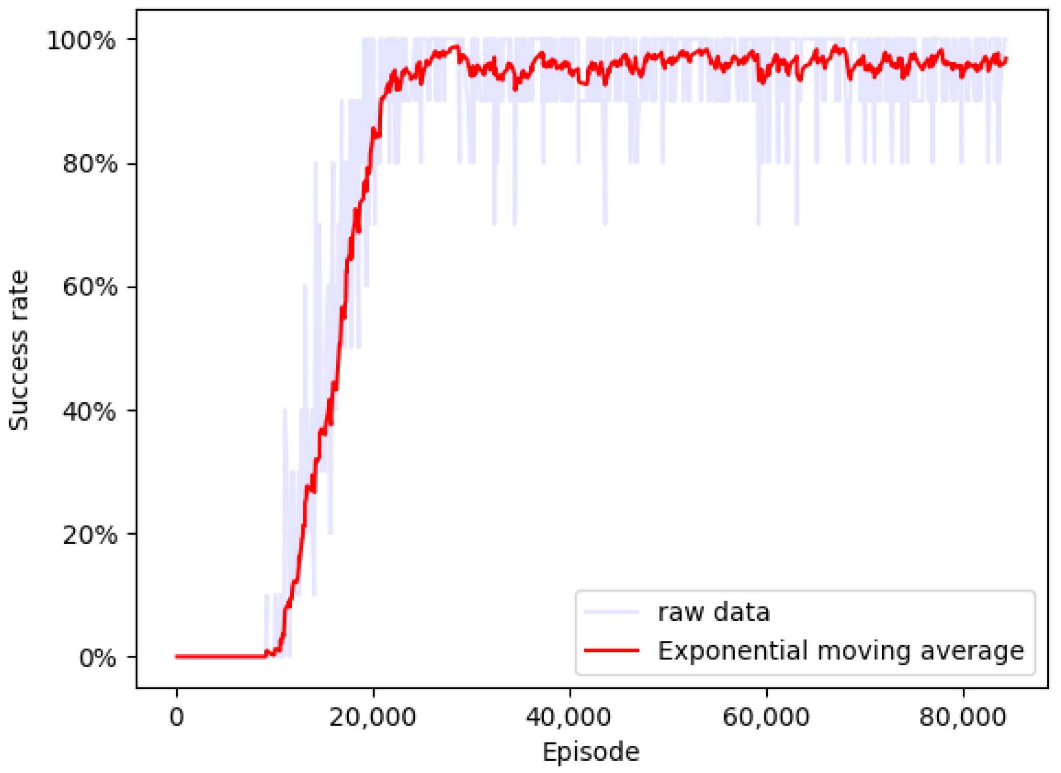
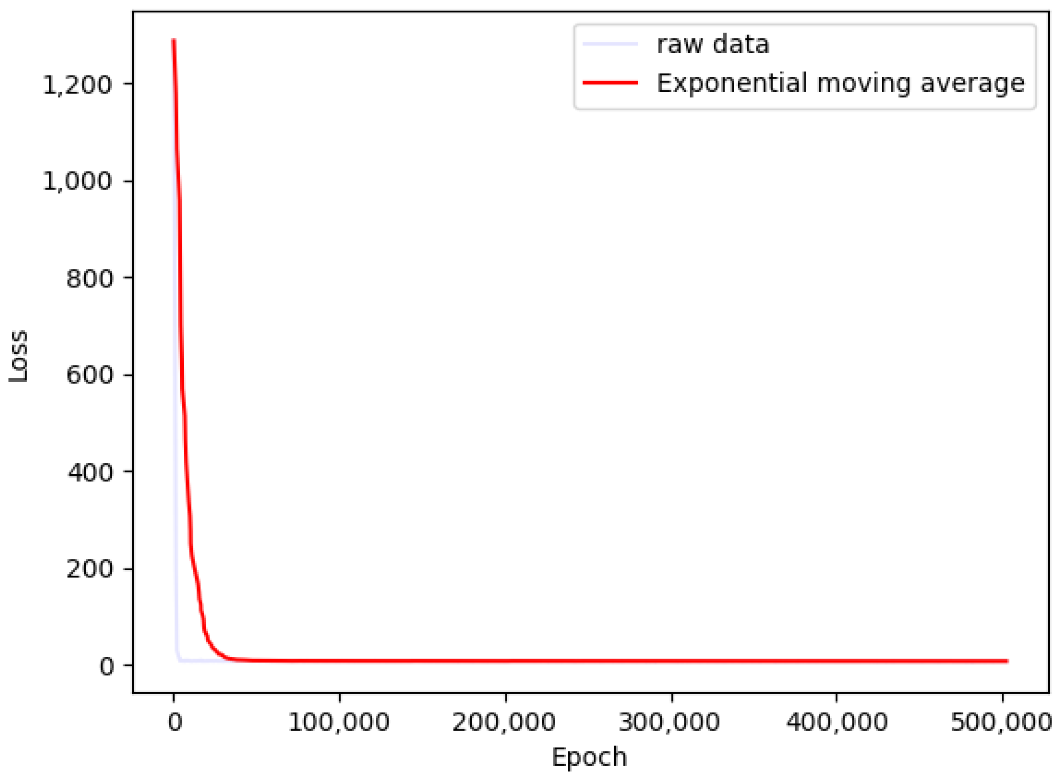
4.1. Simulation
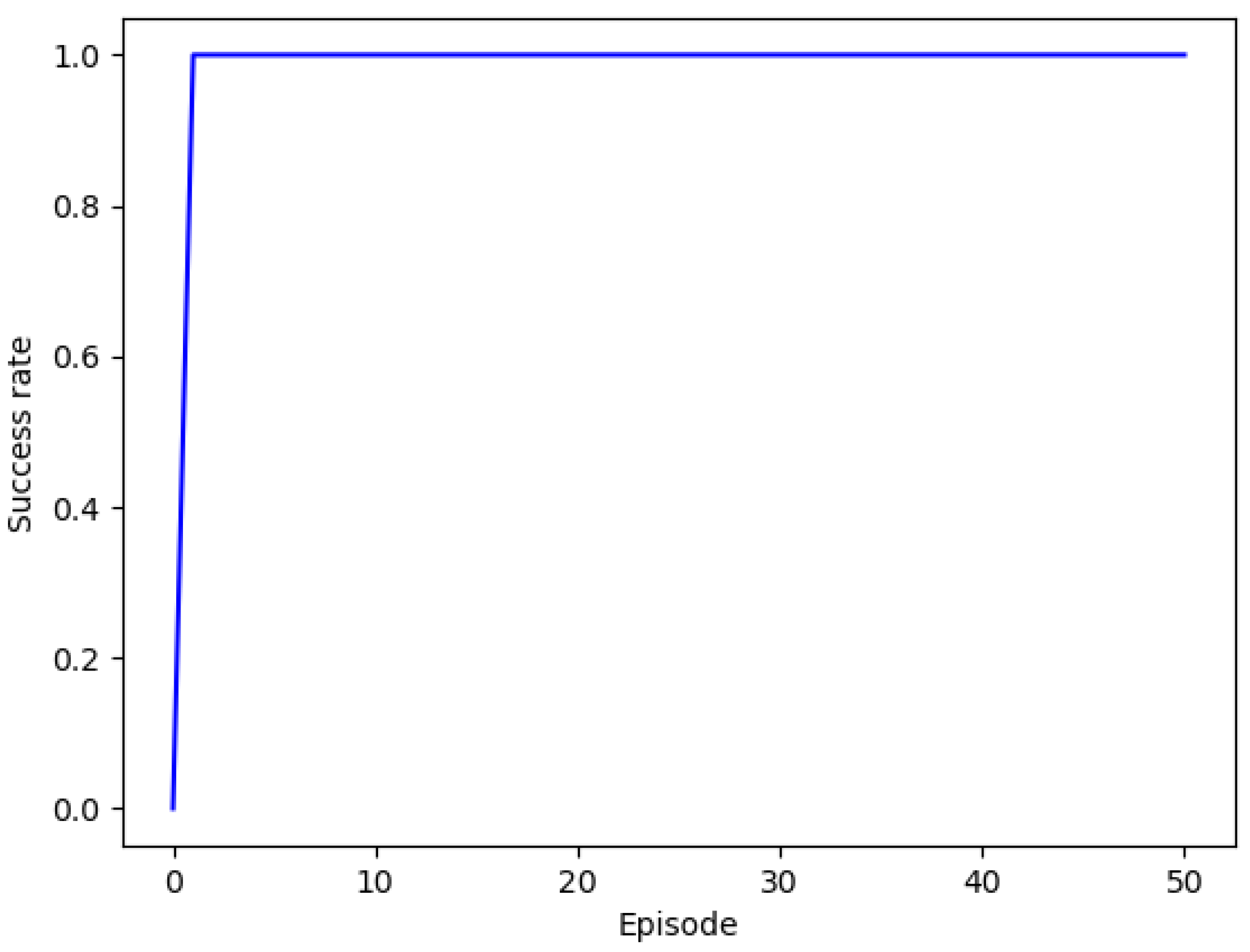
4.2. Experiment
5. Summary and Conclusions
Author Contributions
Funding
Institutional Review Board Statement
Informed Consent Statement
Data Availability Statement
Conflicts of Interest
Abbreviations
| MAMMDP | Multi-Arm Manipulator Markov Decision Process |
| SAC | Soft Actor-Critic |
| HER | Hindsight Experience Replay |
| PRM | Probabilistic Road Map |
| RRT | Rapid exploring Random Trees |
| MDP | Markov Decision Process |
| OBB | Oriented Bounding Boxes |
| LSTM | Long Short-Term Memory |
References
- Berman, S.; Schechtman, E.; Edan, Y. Evaluation of automatic guided vehicle systems. Robot. Comput.-Integr. Manuf. 2009, 25, 522–528. [Google Scholar] [CrossRef]
- Evjemo, L.D.; Gjerstad, T.; Grøtli, E.I.; Sziebig, G. Trends in smart manufacturing: Role of humans and industrial robots in smart factories. Curr. Robot. Rep. 2020, 1, 35–41. [Google Scholar] [CrossRef]
- Arents, J.; Abolins, V.; Judvaitis, J.; Vismanis, O.; Oraby, A.; Ozols, K. Human–robot collaboration trends and safety aspects: A systematic review. J. Sens. Actuator Netw. 2021, 10, 48. [Google Scholar] [CrossRef]
- Spong, M.; Hutchinson, S.; Vidyasagar, M. Robot Modeling and Control; Institute of Electrical and Electronics Engineers Inc.: New York, NY, USA, 2006; Volume 26. [Google Scholar]
- Latombe, J.C. Robot Motion Planning; Kluwer Academic Publishers: Boston, MA, USA, 1991. [Google Scholar]
- Buhl, J.F.; Grønhøj, R.; Jørgensen, J.K.; Mateus, G.; Pinto, D.; Sørensen, J.K.; Bøgh, S.; Chrysostomou, D. A dual-arm collaborative robot system for the smart factories of the future. Procedia Manuf. 2019, 38, 333–340. [Google Scholar] [CrossRef]
- Bonci, A.; Cen Cheng, P.D.; Indri, M.; Nabissi, G.; Sibona, F. Human-robot perception in industrial environments: A survey. Sensors 2021, 21, 1571. [Google Scholar] [CrossRef]
- Pendleton, S.; Andersen, H.; Du, X.; Shen, X.; Meghjani, M.; Eng, Y.; Rus, D.; Ang, M. Perception, planning, control, and coordination for autonomous vehicles. Machines 2017, 5, 6. [Google Scholar] [CrossRef]
- Le, C.H.; Le, D.T.; Arey, D.; Gheorghe, P.; Chu, A.M.; Duong, X.B.; Nguyen, T.T.; Truong, T.T.; Prakash, C.; Zhao, S.T.; et al. Challenges and conceptual framework to develop heavy-load manipulators for smart factories. Int. J. Mechatronics Appl. Mech. 2020, 8, 209–216. [Google Scholar]
- Arents, J.; Greitans, M.; Lesser, B. Construction of a smart vision-guided robot system for manipulation in a dynamic environment. In Artificial Intelligence for Digitising Industry; River Publishers: Gistrup, Denmark, 2022; pp. 205–220. [Google Scholar]
- Hart, P.E.; Nilsson, N.J.; Raphael, B. A formal basis for the heuristic determination of minimum cost paths. IEEE Trans. Syst. Sci. Cybern. 1968, 4, 100–107. [Google Scholar] [CrossRef]
- Karaman, S.; Frazzoli, E. Sampling-based algorithms for optimal motion planning. Int. J. Robot. Res. 2011, 30, 846–894. [Google Scholar] [CrossRef]
- Kavraki, L.E.; Svestka, P.; Latombe, J.C.; Overmars, M.H. Probabilistic roadmaps for path planning in high-dimensional configuration spaces. IEEE Trans. Robot. Autom. 1996, 12, 566–580. [Google Scholar] [CrossRef]
- Zhang, H.Y.; Lin, W.M.; Chen, A.X. Path planning for the mobile robot: A review. Symmetry 2018, 10, 450. [Google Scholar] [CrossRef]
- Schrijver, A. Combinatorial Optimization: Polyhedra and Efficiency; Springer: Berlin/Heidelberg, Germany, 2003; Volume 24. [Google Scholar]
- Kuffner, J.J.; LaValle, S.M. RRT-connect: An efficient approach to single-query path planning. In Proceedings of the 2000 ICRA. Millennium Conference. IEEE International Conference on Robotics and Automation. Symposia Proceedings (Cat. No. 00CH37065), San Francisco, CA, USA, 24–28 April 2000; Volume 2, pp. 995–1001. [Google Scholar]
- Davis, L. Handbook of Genetic Algorithms; CumInCAD: Ljubljana, Slovenia, 1991. [Google Scholar]
- Dorigo, M.; Birattari, M.; Stutzle, T. Ant colony optimization. IEEE Comput. Intell. Mag. 2006, 1, 28–39. [Google Scholar] [CrossRef]
- Kennedy, J.; Eberhart, R. Particle swarm optimization. In Proceedings of the ICNN’95-International Conference on Neural Networks, Perth, WA, Australia, 27 November–1 December 1995; Volume 4, pp. 1942–1948. [Google Scholar]
- Bertsimas, D.; Tsitsiklis, J. Simulated annealing. Stat. Sci. 1993, 8, 10–15. [Google Scholar] [CrossRef]
- Sangiovanni, B.; Rendiniello, A.; Incremona, G.P.; Ferrara, A.; Piastra, M. Deep reinforcement learning for collision avoidance of robotic manipulators. In Proceedings of the 2018 European Control Conference (ECC), Limassol, Cyprus, 12–15 June 2018; pp. 2063–2068. [Google Scholar]
- Prianto, E.; Park, J.H.; Bae, J.H.; Kim, J.S. Deep reinforcement learning-based path planning for multi-arm manipulators with periodically moving obstacles. Appl. Sci. 2021, 11, 2587. [Google Scholar] [CrossRef]
- Zhong, J.; Wang, T.; Cheng, L. Collision-free path planning for welding manipulator via hybrid algorithm of deep reinforcement learning and inverse kinematics. Complex Intell. Syst. 2022, 8, 1899–1912. [Google Scholar] [CrossRef]
- Xie, R.; Meng, Z.; Wang, L.; Li, H.; Wang, K.; Wu, Z. Unmanned aerial vehicle path planning algorithm based on deep reinforcement learning in large-scale and dynamic environments. IEEE Access 2021, 9, 24884–24900. [Google Scholar] [CrossRef]
- Choset, H.M.; Hutchinson, S.; Lynch, K.M.; Kantor, G.; Burgard, W.; Kavraki, L.E.; Thrun, S.; Arkin, R.C. Principles of Robot Motion: Theory, Algorithms, and Implementation; MIT Press: Cambridge, MA, USA, 2005. [Google Scholar]
- Lozano-Perez, T. Spatial planning: A configuration space approach. IEEE Trans. Comput. 1983, C-32, 108–120. [Google Scholar] [CrossRef]
- Laumond, J.P.P. Robot Motion Planning and Control; Springer: Berlin/Heidelberg, Gemany, 1998. [Google Scholar]
- Bergen, G.V.D.; Bergen, G.J. Collision Detection, 1st ed.; Morgan Kaufmann Publishers Inc.: San Francisco, CA, USA, 2003. [Google Scholar]
- Bergen, G.v.d. Efficient collision detection of complex deformable models using AABB trees. J. Graph. Tools 1997, 2, 1–13. [Google Scholar] [CrossRef]
- Ericson, C. Real-Time Collision Detection; CRC Press, Inc.: Boca Raton, FL, USA, 2004. [Google Scholar]
- Fares, C.; Hamam, Y. Collision detection for rigid bodies: A state of the art review. In Proceedings of the GraphiCon 2005—International Conference on Computer Graphics and Vision, Proceedings, Novosibirsk Akademgorodok, Russia, 20–24 June 2005. [Google Scholar]
- Puterman, M.L. Markov Decision Processes: Discrete Stochastic Dynamic Programming, 1st ed.; John Wiley & Sons, Inc.: Hoboken, NJ, USA, 1994. [Google Scholar]
- Sutton, R.S.; Barto, A.G. Reinforcement Learning: An Introduction; A Bradford Book: Cambridge, MA, USA, 2018. [Google Scholar]
- Mnih, V.; Kavukcuoglu, K.; Silver, D.; Rusu, A.A.; Veness, J.; Bellemare, M.G.; Graves, A.; Riedmiller, M.; Fidjeland, A.K.; Ostrovski, G.; et al. Human-level control through deep reinforcement learning. Nature 2015, 518, 529–533. [Google Scholar] [CrossRef]
- Hausknecht, M.; Stone, P. Deep recurrent q-learning for partially observable mdps. In Proceedings of the 2015 AAAI Fall Symposium Series, Arlington, VA, USA, 12–14 November 2015. [Google Scholar]
- Sutton, R.S.; McAllester, D.; Singh, S.; Mansour, Y. Policy Gradient Methods for Reinforcement Learning with Function Approximation. In Proceedings of the 12th International Conference on Neural Information Processing Systems, Cambridge, MA, USA, 29 November–4 December 1999; pp. 1057–1063. [Google Scholar]
- Silver, D.; Lever, G.; Heess, N.; Degris, T.; Wierstra, D.; Riedmiller, M. Deterministic Policy Gradient Algorithms. In Proceedings of the 31st International Conference on International Conference on Machine Learning, Beijing, China, 21–26 June 2014; Volume 32, pp. 387–395. [Google Scholar]
- Lillicrap, T.P.; Hunt, J.J.; Pritzel, A.; Heess, N.; Erez, T.; Tassa, Y.; Silver, D.; Wierstra, D. Continuous control with deep reinforcement learning. In Proceedings of the ICLR (Poster), San Juan, Puerto Rico, 2–4 May 2016. [Google Scholar]
- Mnih, V.; Badia, A.P.; Mirza, M.; Graves, A.; Lillicrap, T.; Harley, T.; Silver, D.; Kavukcuoglu, K. Asynchronous methods for deep reinforcement learning. In Proceedings of the International Conference on Machine Learning. PMLR, New York, NY, USA, 20–22 June 2016; pp. 1928–1937. [Google Scholar]
- Schulman, J.; Levine, S.; Abbeel, P.; Jordan, M.; Moritz, P. Trust region policy optimization. In Proceedings of the International Conference on Machine Learning. PMLR, Lille, France, 7–9 July 2015; pp. 1889–1897. [Google Scholar]
- Schulman, J.; Wolski, F.; Dhariwal, P.; Radford, A.; Klimov, O. Proximal policy optimization algorithms. arXiv 2017, arXiv:1707.06347. [Google Scholar]
- Abdolmaleki, A.; Springenberg, J.T.; Tassa, Y.; Munos, R.; Heess, N.; Riedmiller, M. Maximum a Posteriori Policy Optimisation. In Proceedings of the International Conference on Learning Representations, Vancouver, BC, Canada, 30 April–3 May 2018. [Google Scholar]
- Barth-Maron, G.; Hoffman, M.W.; Budden, D.; Dabney, W.; Horgan, D.; Dhruva, T.; Muldal, A.; Heess, N.; Lillicrap, T. Distributed Distributional Deterministic Policy Gradients. In Proceedings of the International Conference on Learning Representations, Vancouver, BC, Canada, 30 April–3 May 2018. [Google Scholar]
- Schaul, T.; Quan, J.; Antonoglou, I.; Silver, D. Prioritized experience replay. arXiv 2015, arXiv:1511.05952. [Google Scholar]
- Andrychowicz, M.; Wolski, F.; Ray, A.; Schneider, J.; Fong, R.; Welinder, P.; McGrew, B.; Tobin, J.; Pieter Abbeel, O.; Zaremba, W. Hindsight Experience Replay. In Proceedings of the Advances in Neural Information Processing Systems 30, Long Beach, CA, USA, 4–9 December 2017; pp. 5048–5058. [Google Scholar]
- Haarnoja, T.; Zhou, A.; Abbeel, P.; Levine, S. Soft actor-Critic: Off-Policy maximum entropy deep reinforcement learning with a stochastic actor. In Proceedings of the International Conference on Machine Learning, Stockholm, Sweden, 10–15 July 2018; pp. 1861–1870. [Google Scholar]
- Abdel-Nasser, M.; Mahmoud, K. Accurate photovoltaic power forecasting models using deep LSTM-RNN. Neural Comput. Appl. 2019, 31, 2727–2740. [Google Scholar] [CrossRef]
- Gensler, A.; Henze, J.; Sick, B.; Raabe, N. Deep Learning for solar power forecasting—An approach using AutoEncoder and LSTM Neural Networks. In Proceedings of the 2016 IEEE International Conference on Systems, Man, and Cybernetics (SMC), Budapest, Hungary, 9–12 October 2016; pp. 002858–002865. [Google Scholar]
- Ghosh, S.; Vinyals, O.; Strope, B.; Roy, S.; Dean, T.; Heck, L. Contextual lstm (clstm) models for large scale nlp tasks. arXiv 2016, arXiv:1602.06291. [Google Scholar]
- Melamud, O.; Goldberger, J.; Dagan, I. context2vec: Learning generic context embedding with bidirectional lstm. In Proceedings of the 20th SIGNLL Conference on Computational Natural Language Learning, Berlin, Germany, 11–12 August 2016; pp. 51–61. [Google Scholar]
- Choset, H.; Lynch, K.; Hutchinson, S.; Kantor, G.; Burgard, W. Principles of Robot Motion: Theory, Algorithms, and Implementations; Intelligent Robotics and Autonomous Agents Series; MIT Press: Cambridge, MA, USA, 2005. [Google Scholar]
- Latombe, J.C. Robot Motion Planning; Springer Science & Business Media: Berlin/Heidelberg, Germany, 2012; Volume 124. [Google Scholar]
- Fujimoto, S.; Hoof, H.; Meger, D. Addressing function approximation error in actor-critic methods. In Proceedings of the International Conference on Machine Learning, Stockholm, Sweden, 10–15 July 2018; pp. 1582–1591. [Google Scholar]


| Name | Value | Notation | Unit |
|---|---|---|---|
| The number of manipulator joints | 3 | n | pc. (Piece) |
| The number of manipulators | 2 | m | pc. (Piece) |
| Joint maximum | (140, −45, 150, 140, −45, 150) | (Degree) | |
| Joint minimum | (−140, −180, 45, −140, −180, 45) | (Degree) | |
| Dimension of | 6 | Dimension | |
| The number of dynamic obstacle | 1 | pc. (Piece) | |
| The number of past features | 5 | Feature | |
| The number of future features | 3 | Feature | |
| The dynamic obstacle axis |
| Name | Value | Notation | Unit |
|---|---|---|---|
| Policy network size | Node | ||
| Soft Q network size | Node | ||
| Soft value network size | Node | ||
| LSTM network size | Node | ||
| Learning rate | 0.0001 | ||
| Replay memory size | Buffer | ||
| Episode maximum step | 50 | T | Step |
| Soft value target copy rate | 0.005 | ||
| Mini batch size | 512 | m | Batch |
| Environment noise deviation | 0.002 | ||
| Action step size | 0.3813 | ||
| Goal boundary | 0.2 | ||
| Dicount factor | 0.99 | ||
| Entropy temperature parameter | 0.2 |
Publisher’s Note: MDPI stays neutral with regard to jurisdictional claims in published maps and institutional affiliations. |
© 2022 by the authors. Licensee MDPI, Basel, Switzerland. This article is an open access article distributed under the terms and conditions of the Creative Commons Attribution (CC BY) license (https://creativecommons.org/licenses/by/4.0/).
Share and Cite
Park, K.-W.; Kim, M.; Kim, J.-S.; Park, J.-H. Path Planning for Multi-Arm Manipulators Using Soft Actor-Critic Algorithm with Position Prediction of Moving Obstacles via LSTM. Appl. Sci. 2022, 12, 9837. https://doi.org/10.3390/app12199837
Park K-W, Kim M, Kim J-S, Park J-H. Path Planning for Multi-Arm Manipulators Using Soft Actor-Critic Algorithm with Position Prediction of Moving Obstacles via LSTM. Applied Sciences. 2022; 12(19):9837. https://doi.org/10.3390/app12199837
Chicago/Turabian StylePark, Kwan-Woo, MyeongSeop Kim, Jung-Su Kim, and Jae-Han Park. 2022. "Path Planning for Multi-Arm Manipulators Using Soft Actor-Critic Algorithm with Position Prediction of Moving Obstacles via LSTM" Applied Sciences 12, no. 19: 9837. https://doi.org/10.3390/app12199837
APA StylePark, K.-W., Kim, M., Kim, J.-S., & Park, J.-H. (2022). Path Planning for Multi-Arm Manipulators Using Soft Actor-Critic Algorithm with Position Prediction of Moving Obstacles via LSTM. Applied Sciences, 12(19), 9837. https://doi.org/10.3390/app12199837