Article

GisaxStudio—An Open Platform for Analysis and Simulation of GISAXS from 3D Nanoparticle Lattices

1
Faculty of Electrical Engineering and Computing, University of Zagreb, 10000 Zagreb, Croatia
2
Ruđer Bošković Institute, 10000 Zagreb, Croatia
3
Faculty of Science, University of Sarajevo, 71 000 Sarajevo, Bosnia and Herzegovina
*
Author to whom correspondence should be addressed.
Appl. Sci. 2022, 12(19), 9773; https://doi.org/10.3390/app12199773
Submission received: 31 August 2022 / Revised: 26 September 2022 / Accepted: 26 September 2022 / Published: 28 September 2022
(This article belongs to the Topic Advances in Non-Destructive Testing Methods)

Abstract

:

Featured Application

This paper presents the open software platform GisaxStudio for analysis of GISAXS maps from 3D lattices of nanoparticles.

Abstract

Grazing-incidence small-angle X-ray scattering (GISAXS) is a powerful method for the structural analysis of ordered arrays of nanoparticles, quantum dots, or similar objects. However, for the correct interpretation of the measured GISAXS intensity distributions, a proper data analysis, including a suitable model, is required. Here, we demonstrate a software platform, GisaxStudio, aimed at the analysis and simulation of 2D GISAXS intensity distributions from ordered lattices of different nanoparticles. It contains several models that satisfactorily describe the GISAXS from 3D lattices or crystals of nanoparticles prepared by the self-assembly processes, pre-pattering, or ion-beam interaction with the material within their tracks. It also supports different shapes of nanoparticles, including core-shell structure with the center of core possibly displaced from the center of the shell. The software is very useful for fast and accurate GISAXS data analysis.

1. Introduction

The production of materials containing ordered lattices of nanoparticles (NPs) or other nano-objects (NOs) is of great importance today, due to their very interesting properties and many relevant applications in modern nanotechnology [1,2,3]. For example, semiconductor quantum dots (QDs) are the focus of modern science because of their unique optical and electrical properties, tunable by their size and internal structure due to the confinement effects [1,2,3,4,5]. Especially interesting are QDs with a core-shell structure, in which confinement effects are very strong in both the core and the shell [6,7,8,9]. They strongly influence the current carrier and optical properties, ensuring that such materials are highly applicative in solar cells, detectors sensors, and many other devices. Quantum wires (QWs) are another very interesting material due to their specific shape, high surface to volume ratio, and multiple exciton generation effects, which are also highly explored in many photo-sensitive devices [10,11]. As all these properties are highly size- and shape-sensitive, it is very important to develop effective tools for their accurate determination.
In addition to the nanoparticle shape and size, another important factor for the application of such materials is their ordering on the surface or within the matrix. The regular ordering is usually desirable because it allows for controlling the separation of NPs, which greatly influences the material electrical properties. The regularity in ordering can also induce some novel effects in the material, such as mini-band formation, or specific conduction in the desired spatial direction, as well as many others [12,13].
Therefore, the tools for the detailed characterization of size, shape, and arrangement of NPs in a material are of great importance. Grazing-incidence small-angle X-ray scattering (GISAXS) is the leading technique for this purpose because it provides data in reciprocal space with excellent statistics [14,15,16,17,18,19]. The materials with ordered lattices of NPs show characteristic peaks in GISAXS, whose positions and widths are determined by the ordering type of NPs and the degree of regularity in their ordering. Due to that fact, even a visual inspection of the GISAXS map enables a rough estimation of the materials structure, including NP arrangement, separation, and shape. However, for obtaining detailed information about the systems structure, a numerical analysis of a GISAXS map should be performed.
The main problem with the analysis of GISAXS intensity distributions is the proper choice of a model that describes NP ordering, especially the deviations from the ideal NP positions given by the lattice type. The deviations from the ideal NP positions are very important because they significantly affect the position and the width of the peaks in the GISAXS map. Therefore, only the proper choice of the model will lead to the yielding of accurate data from GISAXS analysis. We have analyzed different types of NP ordering in 3D lattices and proposed theoretical models for the description of GISAXS in such systems. These models provide accurate structural data [20]. In another work [21], we have analyzed GISAXS from ion-beam treated materials in which the ion beam forms NPs along its tracks. Finally, some examples are given in [22]. Although these models are published and have proven to be efficient for the analysis of the GISAXS maps, they are usable only by very few experts in GISAXS analysis and modeling. Many users from various disciplines (physics, chemistry, biology, medicine, industry) are in need of the GISAXS technique, but most of them do not know how to analyze the data. Therefore, the software platform which incorporates these models and which is usable by a wide audience is still missing.
Several excellent platforms for description and analysis of GISAXS exist [23,24,25,26,27,28,29], while a full list of the available software for GISAXS analysis can be found in [30]. One of the best known is IsGISAXS [23], aimed at the analysis of different types of islands supported on a substrate. It supports different ordering types of islands, from random distribution via paracrystal, to fully ordered systems. Another frequently used platform is NANOCELL [24], which enables the simulation of 2D diffraction patterns from single-crystals for GISAXS/GISANS geometry. Further, FitGISAXS contains models for the description of GISAXS for monodisperse, polydisperse, and interacting particles with various size distributions, form factors, and structure factors [25]. HipGISAXS is suitable for the treatment of a wide range of structures, shapes, or morphologies, including multilayered polymer films and nanoparticles on top of, or embedded in, a substrate or polymer film layers [26]. DPDAK is a software for the processing and reduction of large amounts of data from synchrotron scattering experiments [27]. It also contains tools for calibration and correction of raw data, one- or two-dimensional integration, and the fitting and further analysis of the data, including the extraction of certain parameters. The most recently developed software is BornAgain, an excellent software for the simulation and fitting of X-ray and neutron reflectometry, off-specular scattering, and grazing-incidence small-angle scattering (GISAS) [28,29]. This platform includes most of the options available in IsGISAXS, along with many new features. BornAgain has a very appealing user-interface and it is, being fairly generic, usable for scientists from different disciplines.
Although currently existing platforms can be used to extract some important features of the 3D assemblies of NPs produced by self-assembly processes, they lack detailed analysis of the NP ordering properties. As stated above, and also discussed in Ref. [20], the NP ordering properties, or more precisely, the type of deviations of the NP positions from the ideal ones, can differ in various spatial directions in the same material. This fact strongly influences the GISAXS intensity distribution, and simulating the intensity distribution by the improper models usually results in incorrect structural parameters, even if the simulated GISAXS map agrees well with the measured one. All things considered, the current software options provide many options, but they are not detailed enough for suitable analysis of the materials based on 3D-ordered NP lattices, nor for specific core-shell structures with the displaced core-shell origins.
In this paper, we present the software platform GisaxStudio for the analysis of thin films consisting of 3D lattices of NPs produced by self-assembled growth or ion-beam irradiation [31]. This software is a result of GISAXS data analysis and suitable model formulation of the aforementioned thin films that has been developed over the last 20 years. It enables the analysis and fitting of 2D GISAXS intensity distributions from 3D NP crystals, 3D lattices of NPs having spheroidal or core-shell shape, and from the NP arrays formed within ion-beam tracks. By fitting of the entire 2D GISAXS map, or even some of its parts, the GisaxStudio enables the determination of the NP’s shape, size, and 3D arrangement properties, including the crystal lattice parameters and disorder type along each of the basis vectors of the 3D lattice. It is also possible to determine statistical distributions of all these parameters. The software includes theoretical models published in [20,21,22], which take into account the NP ordering properties along each of the basis vectors of the 3D NP lattice. The models and the software are already successfully applied in the GISAXS analysis of many systems, including 3D NP lattices [5,7,8,9,11,13,20,21,32,33,34,35,36] and NPs formed within ion tracks [22,37,38,39], where fitting of the full 2D measured map was performed. We show how the platform is constructed, reveal its main features, and demonstrate its performance. The process of preparation for fitting and its main steps are demonstrated. The platform is free for non-commercial use, available at a link given in [31], and is very useful to a broad audience for the analysis of the measured GISAXS maps or for the prediction of measurements using its simulation option.

2. Materials and Methods

GisaxStudio is a modular, multi-platform program for GISAXS analysis of various nanostructured materials. It is written in Java programming language, featuring a graphical user interface (GUI), built-in optimization algorithms, and visualization. It stores all data in the relational database, which facilitates data exchange and reproducibility. Figure 1 shows the architecture of the GisaxStudio application. It is important to note that GisaxStudio has been developed in a modular fashion to enable extendibility and cooperation between the physicist and the computer scientist. Thus, physical models (see Section 3.1) are completely decoupled from the optimization algorithms, GUI, visualization, etc.
Physicists deal only with the models, and in order to produce a new model, they merely provide two Java classes:
  • Parameters class which extends AbstractGisaxsParam and describes the model’s parameters. For instance, instead of the existing iBeam model, suppose our model is a line y = ax + b. The parameter class would then have only two double members: x and y. Members must be annotated in order to expose them to the user via GUI, so that the parameters class would contain simply:
    public class LinearModelParams extends AbstractGisaxsParam {
       @GxParam(defval = 1.00, absLimits = {-1e5, 1e30}, name = "Slope (a)", group
       = "Slope and intercept", tab = "First tab", ordinal = 1)
       public double a;
     
       @GxParam(defval = 0, absLimits = {-1e30, 1e5}, name = "y-intercept (b)",
       group = "Slope and intercept", tab = "First tab", ordinal = 2)
       public double b;
    }
    Through the use of reflection, GisaxStudio will analyze its own code at runtime and dynamically build the GUI dialog for the selected model (e.g., Figure 5a for the iBeam model). Besides primitive types, the parameter class also supports complex numbers, lists of values (manifested as dropdowns for the user), etc. Of course, besides fittable parameters, the parameters class can also include constants and other non-fittable parameters that are easily assigned by the user.
  • Model class, which implements the IGisaxsModel interface, defines 16 methods, the most important being compute(double[]), which computes the model given an array of fittable parameters. In our example, compute would receive a and b via the double array and simply return a*x + b, where x is a vector that has already been assigned:
    @Override
    public double[] compute(double[] params) {
       LinearModelParams pObj = (LinearModelParams)
                    fitVectorToParamObject(params);
       return _xFit
          .times(pObj.a)
          .plus(pObj.b)
          .toArray();
    }
    LinearModel is actually included as a proof-of-concept in the GisaxStudio code, and the code shown above is taken from those two classes (although it is not shown in Figure 1). Helper method fitVectorToParamObject is used to instantiate and populate the params object so that the programmer could use meaningful variable names (a, b) in the code and autocompletion features instead of working with params[0] and params[1].
In conclusion, the physicist deals only with the model and the math, having at their disposal math libraries such as Apache Commons Math [40], ParallelColt [41], and a custom developed matrix and vector library which enables Matlab-like expressions, such as the .times() and .plus() methods shown above. GisaxStudio could be used to fit anything which is manifested/measured as a matrix (image). Apart from these two classes and two parameters in the main application screen (y0 and specular shown in Figure 4), there is nothing GISAXS-specific in the remainder of the application—everything is built dynamically via reflection.
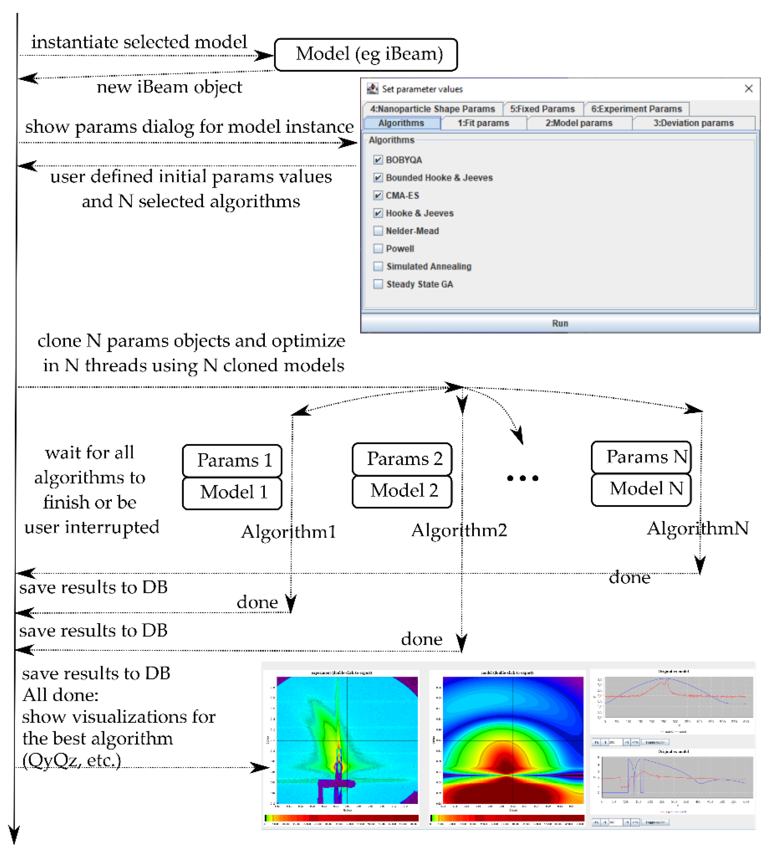
The fitting (optimization) process, whose simplified flow is shown on Figure 2, treats the model as a “black box” and varies the fittable parameters according to some algorithm, calling each time the compute method, in an attempt to find the global minimum in the least squares sense. As GISAXS models are complex and non-linear, it is not reasonable to pick “one best” optimization algorithm. Therefore, in accordance with the generic nature of the application, we have opted for the following approach: GisaxStudio provides a number of different optimization algorithms, and the user can try them all and decide to use those that perform best for their model. Thus, for the time being, the following eight optimization algorithms are included: BobyQA, Bounded Hooke and Jeeves, CMA-ES, Hooke and Jeeves, Nelder–Mead, Powell, Simulated Annealing, and Steady State GA (Figure 2). New algorithms can be easily added, much like the GISAXS model procedure described above: it is simply a matter of implementing the assigned interface and registering the algorithm; the application will then pick up the algorithm and include it in the fitting process.
GisaxStudio instantiates the selected model’s class and retrieves the parameter objects from that instance, which is then inspected via reflection to dynamically build the parameters dialog GUI. This dialog presents the last used values or default values, if it is being used for the first time. After the user sets the initial parameter values and selects the optimization algorithms (e.g., N = 4 in the Figure 2), the application creates N threads, one for each algorithm, provides them with copies of the model and parameters object, and starts the multi-threaded optimization. The main thread receives notifications from the optimization threads and waits for them to finish or to be interrupted by the user. The results are saved in the database as they arrive. Finally, when all the threads are finished, the best optimization result is selected, and a new tab with the visualizations of the winning algorithm, i.e., parameters, is automatically created.
GisaxStudio features a project organization where one project, defined and named by the user, comprises of an arbitrary number of GISAXS images, which are stored in the projects/images subfolder of the application. All other data is stored in a JDBC-compliant (Java DataBase Connectivity) relational database: metadata about the images, regions of interest (ROIs), fits and parameters, results obtained with fits, etc. By default, the portable in-memory H2 Database Engine is used [42], although, any other JDBC-compliant database could be used. Note that a shared environment could also be easily configured by pointing the GisaxStudio to the shared database example, such as PostgreSQL in a local network or shared file system for images. However, for the sake of the simplicity, the default setup is single-user. Such setup allows for portability by simply copying the GisaxStudio folder, which usually contains images and database subfolders, to another computer, even if that computer features a different operating system.

3. Results

3.1. Main Features

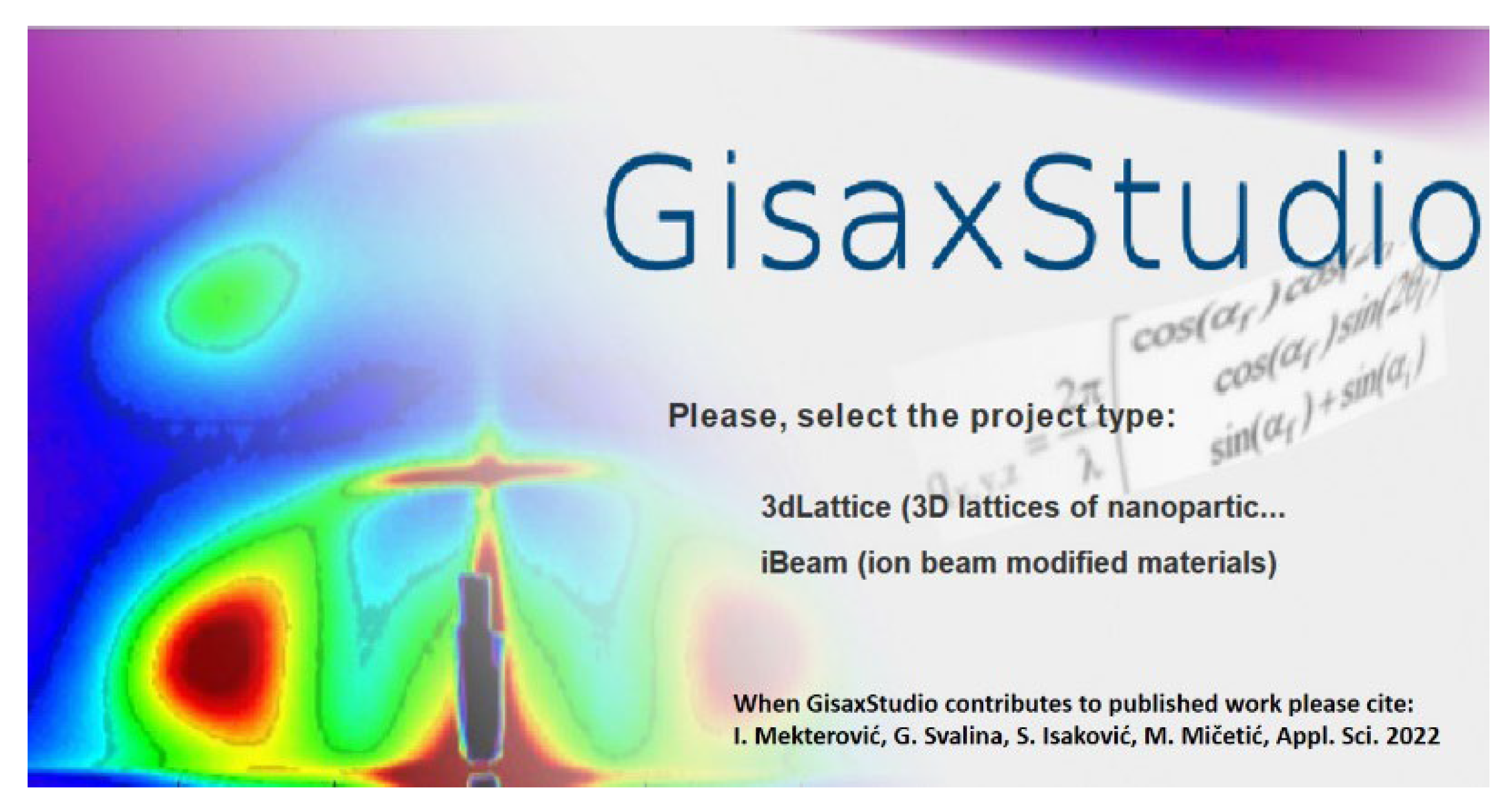
GisaxStudio is a platform for the GISAXS analysis of two types of NP-containing materials: 3D lattices of nanoparticles (experiment type 3dLattice) and ion beam modified materials (iBeam). Figure 3 shows the main window of the software with the choice of the mentioned options. The theory describing the model and functions for the 3dLattice option is published in [20], while the theory for the iBeam option is given in [22].
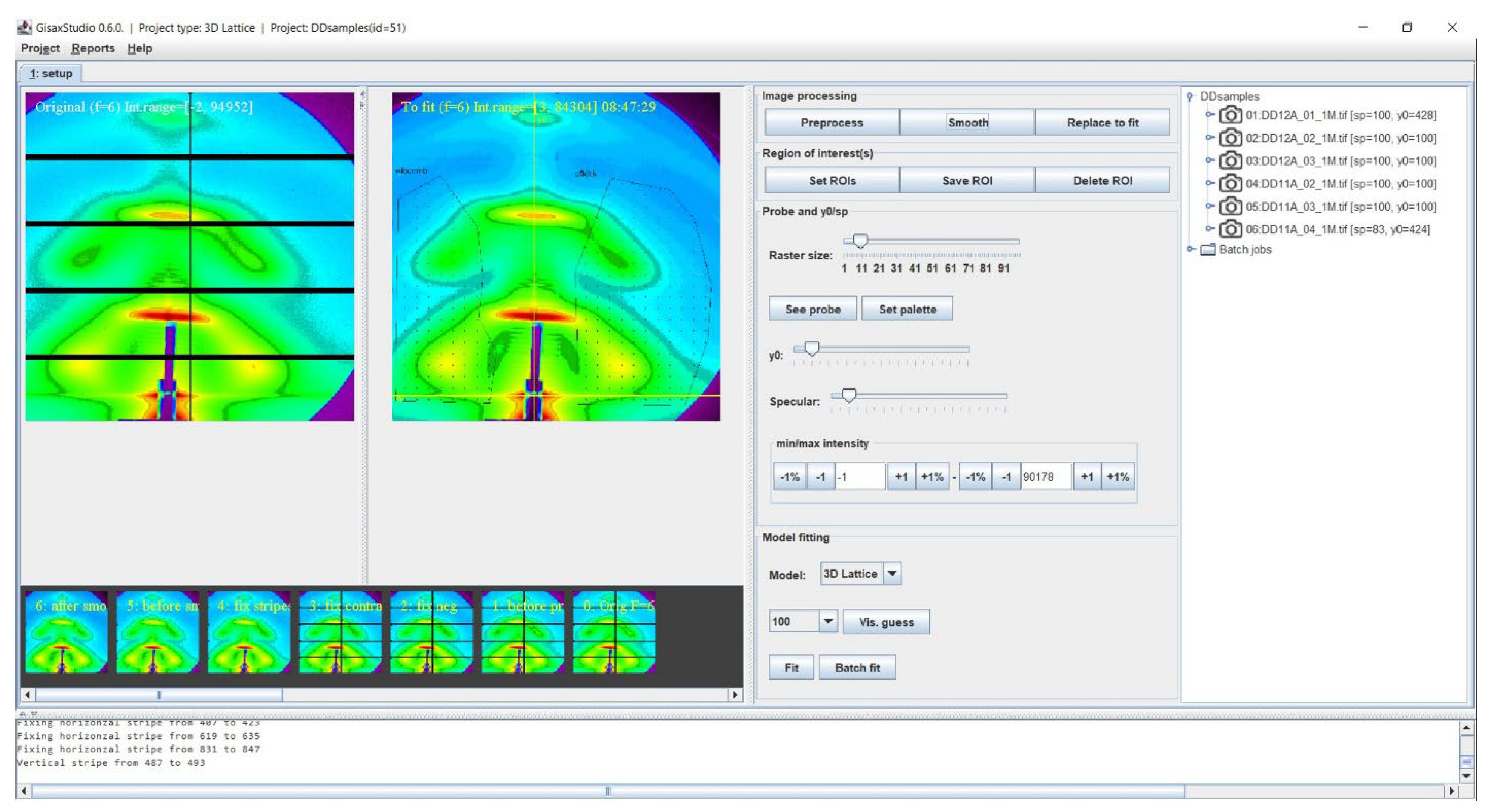
After the project type is chosen, the window (shown in Figure 4) with the main options for the simulation or analysis of the measured GISAXS maps is opened. The tab ‘Project’ enables setting up new project and loading the set of image files that needs to be analyzed, or loading previous projects. The loaded files are displayed at the rightmost column of the window. GisaxStudio enables some simple image processing of the experimental GISAXS maps. For example, the Preprocess button removes the detector’s ‘dead’ lines (black lines in the GISAXS maps), while the Smooth button automatically smooths out the GISAXS map. The Replace to fit button sets the processed image as the one that will be used for further fitting and data analysis. The tab ‘Reports’ provides direct access to the relational database used by the program, so that data can be exported as CSV, and advanced users can even execute custom select and update SQL queries.
One of the main steps in the fitting procedure of the measured data is to choose an arbitrary number of ROIs that will be fitted. ROIs can be chosen using the button Set ROI which opens the open-source ImageJ application incorporated into GisaxStudio. Choosing particular ROIs is required because the measured GISAXS map always contains the contribution of coherent scattering, and it usually contains contributions from the surface roughness close to the Qy = 0 plain, which we do not wish to include in the fit because it cannot be accounted for by the model. In addition, the measured maps often contain some shadows of the vacuum tube, beam-stoppers, or similar items which we do not want to fit. Therefore, we choose the areas of the map (dotted parts in Figure 4) that contain NPs contributions only. These selected parts of the map will be used for fitting.
GisaxStudio enables the simple setting of the incident angle and the lateral beam position directly at the measured map. The y0 parameter, represented by the vertical line on the processed map, should be positioned at the center of the measured signal, while specular (represented by the horizontal line) should be positioned at the reflected beam.

3.2. Visual Estimate Option

In general, a program fits the given set of parameters. These parameters have reasonable defaults set by the GisaxStudio, which can be manually tweaked by the user. Therefore, before the fitting process, it is very useful to use the option Vis guess, which calculates the GISAXS map from the current parameters in the list. The same parameters will be remembered and used as initial parameters for the subsequent fit. This is an optional step, but it enables an experienced user to help the fitting process by moving the initial default parameters closer to the optimal values. The number on the left of the tab ‘Vis Guess’ sets the resolution of the simulated map, as it significantly affects the time needed to calculate the map—lower resolutions will, of course, yield faster results. The window that appears after pressing the Vis guess button is shown in Figure 5. This window allows for setting the desired model and its main parameters. These are specified in six tabs: Fit, Model, Deviation, Nanoparticle shape, Fixed Params, and Experiment Params.
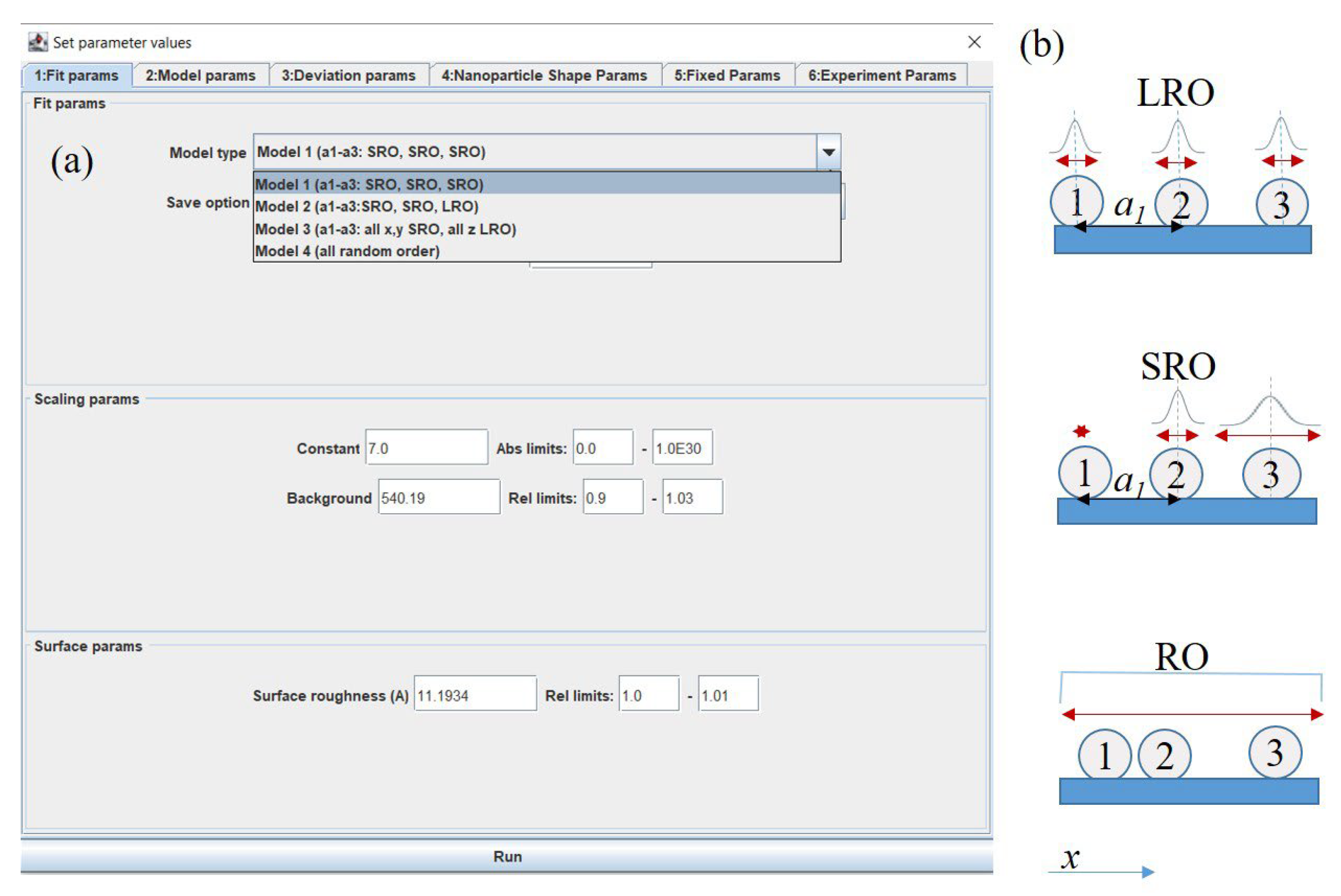
The Fit params tab (Figure 5a) allows us to choose the model most suitable for our system. This tab, in addition to the model, allows us to choose the parameters, including the overall constant, which depends on the intensity collection time, background, and surface roughness of the sample. The choice of the model is crucial for the accuracy of the analysis. Therefore, three main types of the NP ordering, demonstrated in Figure 5b, are available. The program is suitable for the analysis of NP lattices with three basic types of disorder: long range ordering (LRO), short-range ordering (SRO), and random ordering (RO). The disorder describes deviations from the ideal positions of the NPs in a specific 3D lattice. In the LRO model, the positions of the NPs fluctuate around predefined ideal lattice positions, while the separation between the NPs fluctuate in the SRO model. Therefore, the fluctuation probability is increasing from the first to the last NP along the given basis vector. Random ordering shows NP correlations in the NP positions (these are random).
The disorder type can differ in various spatial directions. Because of this, in the description of the 3D lattice, the final model is a combination of three ordering types, which can be different. Each ordering type is associated with one of the three basis vectors that defines the ordering of NP in a 3D lattice, or with some of its components. The model can be set by the variable Model type in the tab ‘Fit parameters’, as shown in Figure 5a. For example, the system that is grown by the self-assembly process, without any restrictions, usually shows SRO in all spatial directions. Therefore, in order to properly describe it, Model 1 (SRO, SRO, SRO) should be chosen. However, for the deposition of NPs in a multilayer, the vertical positions of the layers where the NP form are predefined by the deposition process. Here, the vertical (z component) of all basis vectors should be LRO, while all x, y components that define deviations in the plane within the layers are SRO. Therefore, the appropriate choice for a multilayer system is Model 3 (all x, y SRO, all z LRO). In some cases, the positions of the NPs are predefined along one basis vector (assumed a3). For these types of systems, Model 2 is the appropriate choice. Finally, in some cases, the positions of the NPs are random. In this case, we mainly see, as shown on the GISAXS map, the contribution of the NP shape, and the appropriate choice is Model 4 (all random).
The tab ‘Model params’, shown in Figure 6a, enables setting the lattice type that defines the ideal positions of the NPs in a 3D lattice. The ordering is described by three basis vectors a1a3, whose length and the number of periods along each vector (Nx,y,z) should be specified. The main features of the basis vectors a1a3 are illustrated in Figure 6b, where the body centered tetragonal (BCT) lattice is shown. The presented features are the same for other 3D lattices available in the software. The basis vectors a1 and a2 are in the plane parallel to the films surface/substrate (x-y plane), and they describe the ordering in that plane. The basis vector a3 describes the vertical ordering of the NPs in a 3D lattice. The multilayer period (denoted by vertical period) is given by the z component of basis vector a3. This is well visible in Figure 6c, where a cross-section (x-z plane) through the BCT lattice of the NPs is given.
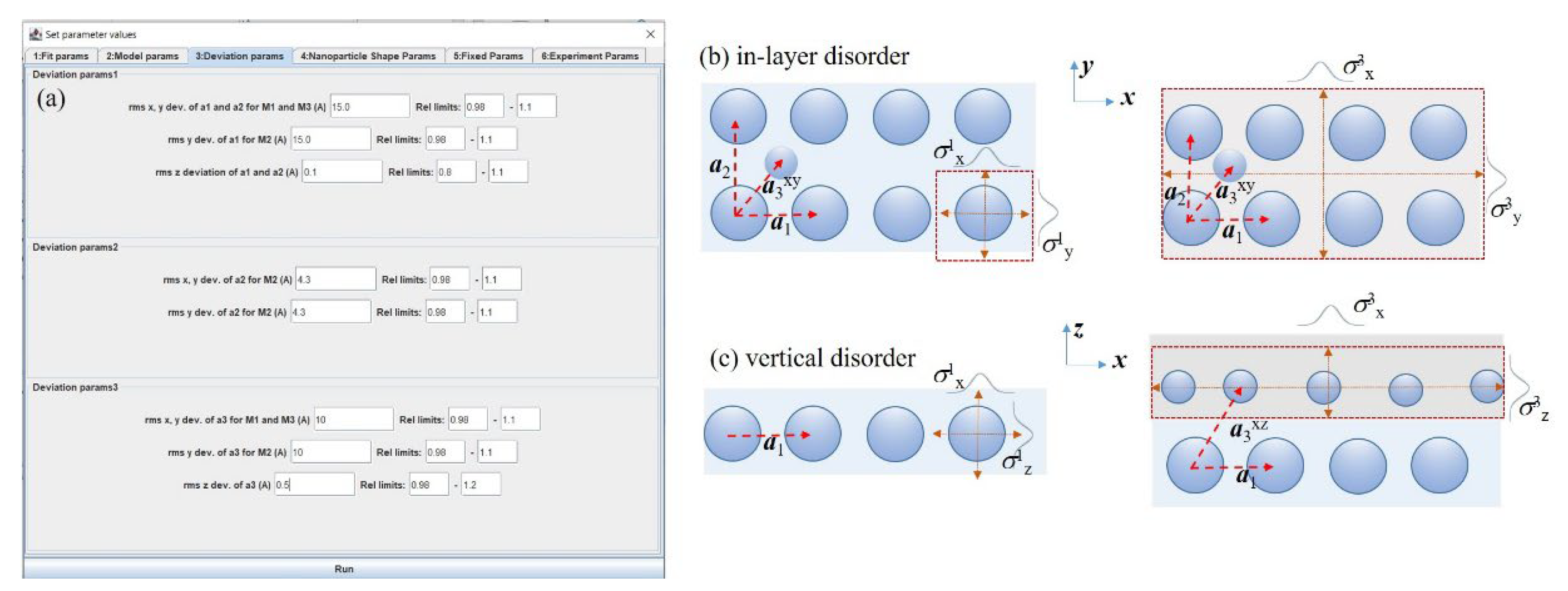
The parameters that describe the disorder of the NP positions, with respect to the ideal positions (given by the basis vectors a1a3), are given in the tab ‘Deviation params’, shown in Figure 7a. The deviations should be set for each spatial direction (x, y, z) of each basis vector. Since the basis vectors a1 and a2 are in the plane parallel to the substrate surface, they usually have the same disorder parameters (σ1,2x,y). Therefore, the software uses the same values of disorder for vectors a1 and a2 in all models, except for Model 2. For Model 2, each basis vector has its own disorder. The drawback is that if the number of fitting parameters is increased, the fitting process becomes more complex. The proper determination of the deviation parameters is often the most difficult step in the fitting process because they strongly influence the shape and width of the GISAXS map peaks caused by the regularity in the NP positions. Figure 7b shows the scheme of the corresponding NP disorder distributions. As mentioned previously, the parameters σ1,2x,y describe disorder in the x-y plane, while the disorder parameters σ3x,y describe the deviations of each new layer of NPs from the ideal position, as illustrated in the right section of Figure 7b. Therefore, these parameters actually define the regularity of the formed 3D lattice, and it is the measure of quality of the self-assembly process in the multilayer deposition preparation method.
The vertical (z) components of disorder σ1,2,3z often have different properties than the lateral components. Here again it is assumed that the disorder related to basis vectors a1 and a2 is the same (σ1z = σ2z). These parameters describe the vertical fluctuation of each NP in a layer parallel to the surface. The parameter σ3z describes the vertical deviation of the entire layer, as illustrated on the right in Figure 7c. If the material is produced by the self-assembly process during multilayer deposition, the vertical disorders σ1,2,3z are usually much smaller than the lateral ones σ1,2,3x,y because the NP forms within the layers of a multilayer. Some examples are given in [20,21].
GisaxStudio currently supports five basic types of the NP shape-structures: sphere, spheroid, ellipsoid, tilted ellipsoid, and core-shell spheroid NPs, as shown in Figure 8. Their parameters can be set in tab ‘Nanoparticle Shape Params’, shown in Figure 8a. The shapes and structures are schematically illustrated in Figure 8b. The main parameters of the NP shape are their radii along the x, y, and z directions Rx,y,z (valid for Ellipsoid). The option Sphere uses only the radius in the x direction (Rx) for all directions, while the option Spheroid uses Rx for radii parallel to the surface and Rz for the direction vertical to the surface. The option Ellipsoid tilted along a3 assumes the same radii values as explained for Ellipsoid, but the entire NP is then assumed to be tilted along the basis vector a3, as shown in Figure 8b.
The option Core-Shell refers to a spheroid with core-shell structure. It consists of different core and shell materials, with radii Rcore and Rshell, respectively. Their origins can be shifted form each other by value d, as shown in Figure 8c. Such structures are often formed by the production of core-shell QDs by thin layer deposition [7,8,9]. The entire system can be scaled in the z direction by factor F, which enables the transition from a spherical to a spheroidal shape. Therefore, actual core-shell radii in the vertical direction are obtained by the multiplication of Rcore and Rshell by factor F.
The distribution of all NP shapes is assumed to be gamma distribution, as described by parameter γ, and the NP radii. All directions are assumed to have the same order of the distribution. The refraction indices of the NPs and their real and imaginary parts should also be set in the ‘Nanoparticle Shape Params’.
The tab Fixed Params includes the refraction indices of the matrix in which the NPs are embedded. It also includes the starting and final averaging angle, along with the step. The averaging is assumed to be performed for the rotation of the 3D lattice around the surface normal (z direction). This is needed because the regular 3D ordering usually appears in domains that are randomly rotated around the surface normal when the material is produced by the self-assembly process. If there is pre-patterning on the substrate that acts as nuclei for the 3D lattice growth, or some other mechanism that predefines the directions of basis vectors a1 and a2, then there is no need for averaging.
The tab Experiment Params contains the details about sample position (sample-detector distance), the vertical position of the primary beam on the detector that may be negative if the beam is below the detector, wavelength of the x-ray beam used for the measurement, and the pixel size.
As previously mentioned, after the parameters in ‘Vis guess’ are set, the Run button activates the calculation of the GISAXS intensity distribution for the given set of parameters. The result appears as a new tab in the application. We recommend running the Vis guess option with different sets of the parameters until the simulated GISAXS map is similar to the measured one. For example, some parameters, such as multilayer period, the NP shape, or NP approximate separation, could be estimated from some other microscopy measurements. After we are satisfied with the Vis guess calculated map, we can start the fitting process.

3.3. Fitting Options

The fitting offers eight different fitting algorithms under the Algorithms tab, as visible in Figure 9a, where one or more options can be chosen for fitting. The other tabs that appear after the Fit button (Figure 4) is clicked contain the same parameters as the Vis guess option. It is important to check the limits for each parameter, which can be set in an absolute or relative fashion. They limit the fitting of the particular parameter. If the limits are too broad, it is more probable that the fitting will go in the wrong direction. On the other hand, if they are too narrow, then the fit will possibly not be able to reach the correct value. However, for most of the parameters, it is possible to estimate the limits correctly. Some of them can be estimated from the GISAXS map, such as the multilayer period, or lateral separation of the NPs (parameter |a1|). The background can also be easily estimated. The width of the Bragg spots related to the 3D lattice formation can be used for the estimation of the disorder parameters. The Vis Guess option is very helpful for this. Setting the limits is very important because the model contains numerous parameters, and many local minima exist in the fitting function. Therefore, if the initial parameters and the limits are not set correctly, it is possible that the fit finishes in some local minima. When the fitting process is started, the software updates the user about the progress of the fit via the status text window, as visible in Figure 9b. We can stop any of the started fitting algorithms at any time using the options stop or kill. Some optimization algorithms can be benignly stopped, and can report the best-found values before they were ended, while others can only be killed, and cannot report any data. Finally, when the fitting procedure is finished, a new tab (Figure 9c) pops up. This tab shows the simulated GISAXS map and the parameters of the fit, along with the line profiles showing the intensity distribution at the chosen cross section.
Finally, the software offers the Batch fit option. Sometimes, fitting can be a time-consuming operation, especially if the number of parameters is large or when user wants to check many variations. In these cases, it is possible to generate an arbitrary number of initial parameter sets (“batch items”), store them in the database, and then launch the batch fitting process, for instance, overnight. Figure 10a shows the dialog for setting the parameters for batch fit. Multiple initial values of each parameter, along with lower and upper limits, can be set by typing in comma delimited values (e.g., “1, 3, 8”), or by using a rudimentary “for-loop” scripting command (e.g., “for( (1, 1); (3, 3); (1, 1) )” that will produce complex numbers “(1, 1), (2, 2), (3, 3)”. Since parallel execution on a desktop or laptop could require too many resources, GisaxStudio will process batch items in a sequential fashion, as follows (Figure 10b):
Repeat until there are unfinished batch items:
load the first unprocessed batch item (parameter set) from list
execute the batch item (fit)
store the results to the database
A beneficial feature of the program is that batch execution can be interrupted at any time and resumed afterwards. For instance, assume that we run a 40-batch item. The program progresses to the, e.g., 20th item, and then the computer powers off (or a user simply kills the program). A total of 19 items have been executed, and their results have been stored in the database. The 20th item was interrupted, and those results are lost. However, when the same batch is run afterwards, it will simply resume from the 20th item and finish the whole batch. When the batch fit is completed, the user can inspect and visualize the results.
In the above text, we have used the option 3dLattice of GisaxStudio. The other option is iBeam, and it has all the same features as 3dLattice, except for the models describing the NP ordering properties within the ion tracks. We have used all the models given in Ref. [22], so we avoid repeating them here.

4. Conclusions

The software platform GisaxStudio, which is aimed at the simulation, analysis, and fitting of GISAXS maps from different types of 2D or 3D lattices of NPs or QDs, is demonstrated. It is specifically developed for GISAXS measured on thin films consisting of 3D lattices of NPs grown by the self-assembly processes, and for the NPs formed within ion-tracks during ion beam irradiation. Therefore, it contains two main groups of models: 3dLattice for application in analysis of GISAXS from NP lattices formed by self-assembled growth, and iBeam aimed at the NPs formed during the ion-beam irradiation of materials. Each group contains several models of the NP arrangement that depend on the material production conditions, i.e., the type of disorder along each of the basis vectors of the formed 3D NP lattice. The main NP shapes supported by GisaxStudio are ellipsoid, spheroid, and sphere with full or core-shell structure. The core-shell structure includes the option of single or double shells, as well as the possibly displaced center of the core with respect to the center of the shell. The models of the NP ordering and their main features available in the software, along with the NP shapes, are discussed. The options for the fitting are provided and supported by examples. The platform is suitable for use by broad audience and non-experts in the GISAXS field.

Author Contributions

Conceptualization M.M.; methodology, I.M. and M.M.; software, I.M.; formal analysis, G.S., S.I. and M.M.; data curation, I.M. and M.M.; writing—review and editing, all authors.; visualization, I.M. and M.M.; project administration, M.M.; funding acquisition, I.M. All authors have read and agreed to the published version of the manuscript.

Funding

This research was funded by the Croatian Science Foundation (no. IP-2018-01-3633) and the European Regional Development Fund under the grant KK.01.1.1.01.0009 (DATACROSS). The authors acknowledge the CERIC-ERIC Consortium for the access to experimental facilities and financial support.

Institutional Review Board Statement

Not applicable.

Informed Consent Statement

Not applicable.

Data Availability Statement

Not applicable.

Acknowledgments

The authors are thankful to J. Erceg for assistance in the sample preparation and D. Mičetić for GISAXS measurements. The authors acknowledge the CERIC-ERIC Consortium for the access to the experimental SAXS facilities and financial support.

Conflicts of Interest

The authors declare no conflict of interest. The funders had no role in the design of the study, in the collection, analyses, or interpretation of data, in the writing of the manuscript, or in the decision to publish the results.

References

  1. Baig, N.; Kammakakam, I.; Falath, W. Nanomaterials: A review of synthesis methods, properties, recent progress, and challenges. Mater. Adv. 2021, 2, 1821–1871. [Google Scholar] [CrossRef]
  2. Chandrakala, V.; Aruna, V.; Angajala, G. Review on metal nanoparticles as nanocarriers: Current challenges and perspectives in drug delivery systems. Emergent Mater. 2022. [Google Scholar] [CrossRef] [PubMed]
  3. de Arquer, F.P.G.; Talapin, D.V.; Klimov, V.I.; Arakawa, Y.; Bayer, M.; Sargent, E.H. Semiconductor quantum dots: Technological progress and future challenges. Science 2021, 373, eaaz8541. [Google Scholar] [CrossRef]
  4. Ossicini, S.; Amato, M.; Guerra, R.; Palummo, M.; Pulci, O. Silicon and Germanium Nanostructures for Photovoltaic Applications: Ab-Initio Results. Nanoscale Res. Lett. 2010, 5, 1637–1649. [Google Scholar] [CrossRef]
  5. Nekić, N.; Šarić, I.; Salamon, K.; Basioli, L.; Sancho-Parramon, J.; Grenzer, J.; Hübner, R.; Bernstorff, S.; Petravić, M.; Mičetić, M. Preparation of non-oxidized Ge quantum dot lattices in amorphous Al2O3, Si3N4 and SiC matrices. Nanotechnology 2019, 30, 335601. [Google Scholar] [CrossRef] [PubMed]
  6. de Oliveira, E.L.; Albuquerque, E.L.; de Sousa, J.S.; Farias, G.A.; Peeters, F.M. Configuration-Interaction Excitonic Absorption in Small Si/Ge and Ge/Si Core/Shell Nanocrystals. J. Phys. Chem. C 2012, 116, 4399–4407. [Google Scholar] [CrossRef]
  7. Nekić, N.; Sancho-Parramon, J.; Radovic, I.B.; Grenzer, J.; Huebner, R.; Bernstorff, S.; Ivanda, M.; Buljan, M. Ge/Si core/shell quantum dots in alumina: Tuning the optical absorption by the core and shell size. Nanophotonics 2017, 6, 1055–1062. [Google Scholar] [CrossRef]
  8. Buljan, M.; Radić, N.; Sancho-Paramon, J.; Janicki, V.; Grenzer, J.; Radovic, I.B.; Siketić, Z.; Ivanda, M.; Utrobičić, A.; Hübner, R.; et al. Production of three-dimensional quantum dot lattice of Ge/Si core–shell quantum dots and Si/Ge layers in an alumina glass matrix. Nanotechnology 2015, 26, 065602. [Google Scholar] [CrossRef]
  9. Basioli, L.; Sancho-Parramon, J.; Despoja, V.; Fazinić, S.; Radović, I.B.; Mihalić, I.B.; Salamon, K.; Nekić, N.; Ivanda, M.; Dražić, G.; et al. Ge Quantum Dots Coated with Metal Shells (Al, Ta, and Ti) Embedded in Alumina Thin Films for Solar Energy Conversion. ACS Appl. Nano Mater. 2020, 3, 8640–8650. [Google Scholar] [CrossRef]
  10. Kes, H.; Okan, S.; Aktas, S. The excitons in infinite potential centered multilayered coaxial quantum wire and the magnetic field effects on their properties. Superlattices Microstruct. 2020, 139, 106421. [Google Scholar] [CrossRef]
  11. Basioli, L.; Tkalčević, M.; Bogdanović-Radović, I.; Dražić, G.; Nadazdy, P.; Siffalovic, P.; Salamon, K.; Mičetić, M. 3D Networks of Ge Quantum Wires in Amorphous Alumina Matrix. Nanomaterials 2020, 10, 1363. [Google Scholar] [CrossRef] [PubMed]
  12. Lazarenkova, O.L.; Balandin, A.A. Miniband formation in a quantum dot crystal. J. Appl. Phys. 2001, 89, 5509–5515. [Google Scholar] [CrossRef]
  13. Buljan, M.; Roshchupkina, O.; Šantić, A.; Holý, V.; Baehtz, C.; Mücklich, A.; Horák, L.; Valeš, V.; Radić, N.; Bernstorff, S.; et al. Growth of a three-dimensional anisotropic lattice of Ge quantum dots in an amorphous alumina matrix. J. Appl. Crystallogr. 2013, 46, 709–715. [Google Scholar] [CrossRef]
  14. Müller-Buschbaum, P. A Basic Introduction to Grazing Incidence Small-Angle X-Ray Scattering. In Applications of Synchrotron Light to Scattering and Diffraction in Materials and Life Sciences; Lecture Notes in Physics; Chapter 3; Springer: Berlin/Heidelberg, Germany, 2009; pp. 61–89. [Google Scholar] [CrossRef]
  15. Renaud, G.; Lazzari, R.; Leroy, F. Probing surface and interface morphology with Grazing Incidence Small Angle X-Ray Scattering. Surf. Sci. Rep. 2009, 64, 255–380. [Google Scholar] [CrossRef]
  16. Cristofolini, L. Synchrotron X-ray techniques for the investigation of structures and dynamics in interfacial systems. Curr. Opin. Colloid Interface Sci. 2014, 19, 228–241. [Google Scholar] [CrossRef]
  17. Hexemer, A.; Müller-Buschbaum, P. Advanced grazing-incidence techniques for modern soft-matter materials analysis. IUCrJ 2015, 2, 106–125. [Google Scholar] [CrossRef]
  18. Müller-Buschbaum, P. GISAXS and GISANS as metrology technique for understanding the 3D morphology of block copolymer thin films. Eur. Polym. J. 2016, 81, 470–493. [Google Scholar] [CrossRef]
  19. Smilgies, D. GISAXS: A versatile tool to assess structure and self-assembly kinetics in block copolymer thin films. J. Appl. Polym. Sci. 2021, 60, 1023–1041. [Google Scholar] [CrossRef]
  20. Buljan, M.; Radić, N.; Bernstorff, S.; Dražić, G.; Bogdanović-Radović, I.; Holý, V. Grazing-incidence small-angle X-ray scattering: Application to the study of quantum dot lattices. Acta Crystallogr. Sect. A Found. Crystallogr. 2012, 68, 124–138. [Google Scholar] [CrossRef] [Green Version]
  21. Basioli, L.; Salamon, K.; Tkalčević, M.; Mekterović, I.; Bernstorff, S.; Mičetić, M. Application of GISAXS in the Investigation of Three-Dimensional Lattices of Nanostructures. Crystals 2019, 9, 479. [Google Scholar] [CrossRef]
  22. Buljan, M.; Karlušić, M.; Nekić, N.; Jerčinović, M.; Bogdanović-Radović, I.; Bernstorff, S.; Radić, N.; Mekterović, I. GISAXS analysis of ion beam modified films and surfaces. Comput. Phys. Commun. 2017, 212, 69–81. [Google Scholar] [CrossRef]
  23. Lazzari, R. IsGISAXS: A program for grazing-incidence small-angle X-ray scattering analysis of supported islands. J. Appl. Crystallogr. 2002, 35, 406–421. [Google Scholar] [CrossRef]
  24. Tate, M.P.; Urade, V.N.; Kowalski, J.D.; Wei, T.-C.; Hamilton, B.D.; Eggiman, B.W.; Hillhouse, H.W. Simulation and Interpretation of 2D Diffraction Patterns from Self-Assembled Nanostructured Films at Arbitrary Angles of Incidence: From Grazing Incidence (Above the Critical Angle) to Transmission Perpendicular to the Substrate. J. Phys. Chem. B 2006, 110, 9882–9892. [Google Scholar] [CrossRef]
  25. Babonneau, D. FitGISAXS: Software package for modelling and analysis of GISAXS data using IGOR Pro. J. Appl. Crystallogr. 2010, 43, 929–936. [Google Scholar] [CrossRef]
  26. Chourou, S.T.; Sarje, A.; Li, X.S.; Chan, E.R.; Hexemer, A. HipGISAXS: A high-performance computing code for simulating grazing-incidence X-ray scattering data. J. Appl. Crystallogr. 2013, 46, 1781–1795. [Google Scholar] [CrossRef]
  27. Benecke, G.; Wagermaier, W.; Li, C.; Schwartzkopf, M.; Flucke, G.; Hoerth, R.; Zizak, I.; Burghammer, M.; Metwalli, E.; Müller-Buschbaum, P.; et al. A customizable software for fast reduction and analysis of large X-ray scattering data sets: Applications of the new DPDAK package to small-angle X-ray scattering and grazing-incidence small-angle X-ray scattering. J. Appl. Crystallogr. 2014, 47, 1797–1803. [Google Scholar] [CrossRef]
  28. Durniak, C.; Ganeva, M.; Pospelov, G.; Van Herck, W.; Wuttke, J. BornAgain—Software for Simulating and Fitting X-ray and Neutron Small-Angle Scattering at Grazing Incidence. In Proceedings of the 26th International Conference on Amorphous and Nanocrystalline Semiconductors, Aachen, Germany, 13–18 September 2015; Available online: http://juser.fz-juelich.de/record/255761 (accessed on 28 August 2022).
  29. Pospelov, G.; Van Herck, W.; Burle, J.; Loaiza, J.M.C.; Durniak, C.; Fisher, J.M.; Ganeva, M.; Yurov, D.; Wuttke, J. BornAgain: Software for simulating and fitting grazing-incidence small-angle scattering. J. Appl. Crystallogr. 2020, 53, 262–276. [Google Scholar] [CrossRef]
  30. Available online: http://gisaxs.com/index.php/Software/ (accessed on 21 September 2022).
  31. GisaxStudio. Available online: http://homer.zpr.fer.hr/gisaxstudio/ (accessed on 30 August 2022).
  32. Tkalčević, M.; Boršćak, D.; Periša, I.; Bogdanović-Radović, I.; Janković, I.; Petravić, M.; Bernstorff, S.; Mičetić, M. Multiple Exciton Generation in 3D-Ordered Networks of Ge Quantum Wires in Alumina Matrix. Materials 2022, 15, 5353. [Google Scholar] [CrossRef]
  33. Shaji, A.; Micetic, M.; Halahovets, Y.; Nadazdy, P.; Matko, I.; Jergel, M.; Majkova, E.; Siffalovic, P. Real-time tracking of the self-assembled growth of a 3D Ge quantum dot lattice in an alumina matrix. J. Appl. Crystallogr. 2020, 53, 1029–1038. [Google Scholar] [CrossRef]
  34. Tkalčević, M.; Basioli, L.; Salamon, K.; Šarić, I.; Parramon, J.S.; Bubaš, M.; Bogdanović-Radović, I.; Bernstorff, S.; Fogarassy, Z.; Balázsi, K.; et al. Ge quantum dot lattices in alumina prepared by nitrogen assisted deposition: Structure and photoelectric conversion efficiency. Sol. Energy Mater. Sol. Cells 2020, 218, 110722. [Google Scholar] [CrossRef]
  35. Krause, M.; Buljan, M.; Mücklich, A.; Möller, W.; Fritzsche, M.; Facsko, S.; Heller, R.; Zschornak, M.; Wintz, S.; Endrino, J.L.; et al. Compositionally modulated ripples during composite film growth: Three-dimensional pattern formation at the nanoscale. Phys. Rev. B 2014, 89, 085418. [Google Scholar] [CrossRef]
  36. Karlušić, M.; Mičetić, M.; Kresić, M.; Jakšić, M.; Šantić, B.; Bogdanović-Radović, I.; Bernstorff, S.; Lebius, H.; Ban-D’Etat, B.; Rožman, K.; et al. Nanopatterning surfaces by grazing incidence swift heavy ion irradiation. Appl. Surf. Sci. 2021, 541, 148467. [Google Scholar] [CrossRef]
  37. Karlušić, M.; Bernstorff, S.; Siketić, Z.; Šantić, B.; Bogdanović-Radović, I.; Jakšić, M.; Schleberger, M.; Buljan, M. Formation of swift heavy ion tracks on a rutile TiO2 (001) surface. J Appl Crystallogr. 2016, 49, 1704–1712. [Google Scholar] [CrossRef] [PubMed]
  38. Radović, I.B.; Buljan, M.; Karlušić, M.; Jerčinović, M.; Dražič, G.; Bernstorff, S.; Boettger, R. Modification of semiconductor or metal nanoparticle lattices in amorphous alumina by MeV heavy ions. New J. Phys. 2016, 18, 093032. [Google Scholar] [CrossRef]
  39. Karlušić, M.; Kozubek, R.; Lebius, H.; Ban-D’Etat, B.; Wilhelm, R.A.; Buljan, M.; Siketić, Z.; Scholz, F.; Meisch, T.; Jakšić, M.; et al. Response of GaN to energetic ion irradiation: Conditions for ion track formation. J. Phys. D: Appl. Phys. 2015, 48, 325304. [Google Scholar] [CrossRef] [Green Version]
  40. Commons Math: The Apache Commons Mathematics Library. Available online: https://commons.apache.org/proper/commons-math/ (accessed on 30 August 2022).
  41. Parallel Colt. A Multithreaded Version of Colt—A library for High Performance Scientific Computing in JAVA. Available online: https://github.com/rwl/ParallelColt (accessed on 30 August 2022).
  42. H2 Database Engine. Available online: https://www.h2database.com/ (accessed on 30 August 2022).
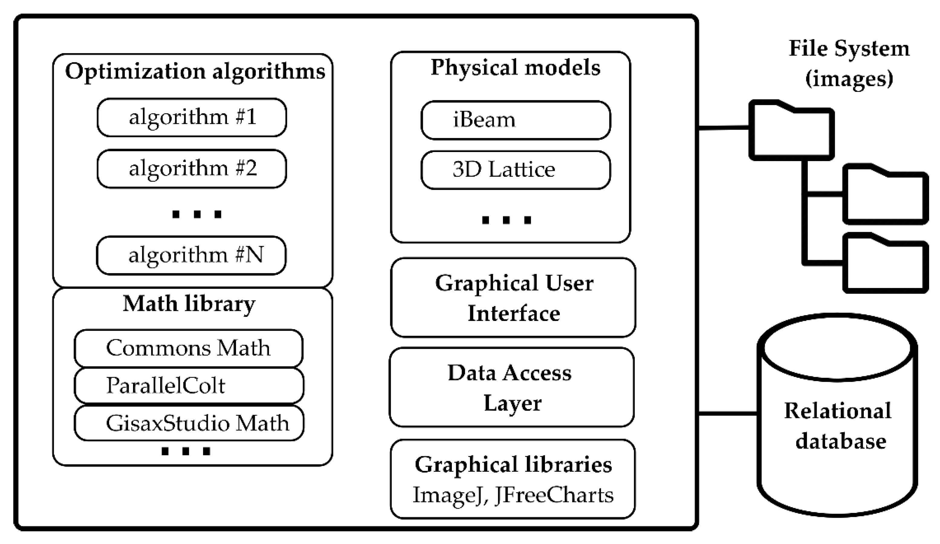
Figure 1. GisaxStudio architecture. Physical models are decoupled from the generic optimization algorithms. Images are stored in file system, and project data is stored in a JDBC-compliant relational database.
Applsci 12 09773 g001
Figure 2. Fitting procedure in GisaxStudio: after the user selects the model and assigns initial values of the corresponding model, the application spawns N threads (corresponding to the number of chosen optimization algorithms) and initiates a multi-threaded optimization. When all the threads are finished (or interrupted by the user), the application visualizes the resulting winning algorithms.
Applsci 12 09773 g002
Figure 3. Starting window of GisaxStudio enabling the choice of the experiment type: the 3dLattice option should be used for the analysis of GISAXS from 3D ordered lattices of NPs, while iBeam is aimed at the analysis of NPs formed within ion-beam induced tracks.
Applsci 12 09773 g003
Figure 4. Window for setup the analysis options for 3dLattice experiment type. It contains the GISAXS map which should be analysed, as well as the options for image processing and simulation in the middle columns, followed by the list of loaded files in the current project on the right side.
Applsci 12 09773 g004
Figure 5. (a) Window for setting the parameter values that appears for the ‘Vis Guess’ option in the main window. The opened window contains six tabs: Fit, Model, Deviation, Nanoparticle shape, Fixed params and Experiment params. The chosen tab allows for setting the model type, scaling, and surface parameters. (b) Scheme of possible ordering types along one of the basis vectors (a1) of the NP lattice: long range ordering (LRO), short-range ordering (SRO), and random ordering (RO).
Applsci 12 09773 g005
Figure 6. (a) Tab Model params with the corresponding parameters describing the lattice type and its main parameters. (b) Scheme of ordering in a body centered tetragonal (BCT) lattice defined by basis vectors a1a3. (c) Cross-section of the 3D lattice of NPs having BCT unit cell with N1 = 6 and N3 = 4 periods along basis vectors a1 and a3, respectively.
Applsci 12 09773 g006
Figure 7. (a) Tab Deviation params with the corresponding parameters. (b) Illustration of disorder parameters σ1,2,3xy. The disorder properties within each layer parallel to the surface (σ1,2xy) are usually the same (left), and they describe the deviations of each NP within a layer from the ideal positions. The parameters σ3xy (right) describe the disorder of each layer from the ideal position, and therefore, are a measure of the quality of the self-assembly process that leads to formation of the 3D NP lattice. (c) The disorder parameters in the vertical direction (perpendicular to the surface). These parameters describe the deviation of each NP within a layer (σ1,2z), and of each layer (σ3z) from the ideal positions in the vertical (z) direction.
Applsci 12 09773 g007
Figure 8. (a) Tab Nanoparticle Shape Params and its parameters. (b) Some of NP shapes currently available in the software: spheroid defined by lateral (in x-y plane) and vertical (z direction) radii Rx and Rz, respectively. Option Ellipsoid has the additional radius Ry in the y direction; tilted ellipsoid with the tilt along basis vector a3. (c) Core-shell spheroid with the core and shell radii Rcore and Rshell, respectively, and the shift of the shell origin d. The spheroidal shape is defined by factor F, so that the actual vertical radii are the product of Rcore and Rshell and factor F.
Applsci 12 09773 g008
Figure 9. Tabs related to the fitting of the 2D GISAXS map. (a) The window with fitting parameters, including the same parameters as in Vis guess option and an additional Algorithms tab that enables the choice of the fitting algorithms. (b) Window that appears after starting of the fit, showing its progress. After the fitting is finished, the parameters are shown in the window at the bottom. (c) Results of the fitting process, including the original and simulated GISAXS map using the best-fit parameters, along with the line profiles at the right.
Applsci 12 09773 g009
Figure 10. (a) Tab related to Batch fit option. (b) Start or delete options of Batch fit in the main window.
Applsci 12 09773 g010
Publisher’s Note: MDPI stays neutral with regard to jurisdictional claims in published maps and institutional affiliations.