Abstract
When collecting dust samples from coal-fired power plant chimneys, a nozzle specially designed with an inlet shape of circle type is used for constant velocity suction. However, it is cumbersome to use nozzles with different areas depending on the flow rate. In this study, the effect of the nozzle inlet shape of the isokinetic sampler on the performance of constant velocity suction was evaluated through simulation. The simulations were conducted using the realizable k−ε model, which is known to be suitable for separation flow analysis for particles of 1–50 μm. The turbulent flow fully developed before reaching the inlet of the sampling probe, and the flow rate was set under the condition that the uniformity was secured at approximately 92% at least. The aspiration ratio was employed for evaluating the degree of constant velocity aspiration of the isokinetic sampling probe. It was found that the larger the particle diameter and the faster the flow rate, the larger the aspiration ratio for both the circular and ellipsoidal inlets. In particular, compared with the circular inlet, the aspiration ratio of the sampler with ellipsoidal inlet was closer to 1 in the free-flow velocity range, from 5 to 15 m/s. For this reason, if the ellipsoidal inlet nozzle is used by adjusting only the length parallel to the major axis, the maintenance cost is expected to be reduced compared to the circle-type nozzle.
1. Introduction
Ultrafine particles (PM2.5) having a diameter of 2.5 μm or below are known to cause respiratory diseases in certain vulnerable social groups such as the elderly and infants [1]. In particular, smaller particles are more likely to be toxic and can penetrate deeply into the lung, thus inducing serious health issues, including respiratory and cardiovascular diseases, reproductive and central nervous system dysfunction, and even cancer [2,3]. Therefore, it is crucial to real-time monitor the air quality in industrial areas, where numerous businesses emit airborne pollutants, as well as in residential and commercial areas, which have high population densities. Particulate matter concentrations are provided to the public on a daily basis [4]. Accordingly, pollutant emission standards are becoming stricter worldwide in order to reduce the effects of particulate matter on air pollution [5]. In particular, dust concentration must be monitored in real time at large air-pollutant-emitting facilities such as coal-fired power plants [6]. In general, the light-transmission method is used to measure the dust concentration in the chimney of a coal-fired power plant. This method involves measuring the degree of change in light intensity owing to foreign substances such as dust in the exhaust gas when light is transmitted from a light source installed in one side of the chimney to the detector installed on the opposite side; this light-intensity change is then converted into a concentration [7].
Coal-fired power plants are also investing in the reduction of air pollutants. The emission concentration of discharged dust is strictly monitored by a telemonitoring system (TMS) using the light-transmission method, which is used in conjunction with an electrostatic precipitator [8]; in general, the accuracy of dust concentration measurements is determined via the error rates of the semi-automatic method and light transmission method used by the TMS. Since the semi-automatic method utilizes a sampler to ensure that the sampling nozzle and flow direction within a power-plant chimney are aligned parallel to each other, it is important to minimize the effect of exhaust gas flow during isokinetic sampling [9].
Particles gain an inertial force as they move along the flow direction, and the degree of isokinetic sampling is determined according to free-stream and sampling flow velocity [10]. Figure 1a shows the super-isokinetic sampling of particles when the velocity inside the sampler is faster than that of the free stream, which results in greater inertia of the particles. By contrast, Figure 1c shows the case of sub-isokinetic sampling of particles along the flow arising from the slower velocity of the particles inside the sampler compared with the particles in the free stream. As shown in Figure 1b, an accurate particle concentration can be obtained only from isokinetic sampling [11]. Therefore, typical sampling of an aerosol can be performed, and pollutants can be effectively controlled by developing an isokinetic sampler [12].
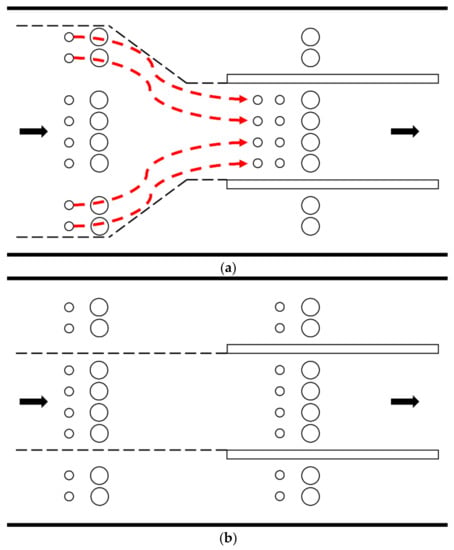

Figure 1.
Isokinetic sampling condition classification: (a) super-isokinetic sampling, (b) isokinetic sampling, and (c) sub-isokinetic sampling.
The aspiration ratio, i.e., the ratio of the particle number concentration measured in a free stream to the particle number concentration measured at the sampling probe inlet, is one of the indicators for evaluating the accuracy of isokinetic sampling of an aerosol. An aspiration ratio closer to 1 indicates that the sampling probe is effectively performing isokinetic sampling [13].
The geometric structure of a sampling probe can significantly impact the particle distribution [14]. The major causes of distortion of the aerosol in the sampling nozzle area include the formation of vena contracta as a result of the impact against the nozzle wall owing to turbulence, gravity sedimentation, and electrostatic interaction [15]. If the velocity vectors governing the free stream and flow suctioned into the sampling probe vary significantly, extracting representative samples becomes difficult, and the suctioned sample may underestimate or overestimate the actual concentration [16]. Therefore, the inlet tip of a sampling probe must be designed so that the effects on aerosol behavior are minimized, as the sampling nozzle shape of an isokinetic sampler affects the flow pattern around the nozzle.
In recent studies on an isokinetic sampler, its sampling performance was improved using a probe and shroud arranged on the co-axis. The particle number concentration is considerably affected by the free-stream velocity around the sampling probe inlet as well as the sampling conditions, and thus the shroud reduces the flow velocity before the flow reaches the inlet of the sampling nozzle, thus enabling isokinetic sampling irrespective of the velocity of a wide free-stream [17]. Furthermore, in a shrouded isokinetic probe, the wall loss is lower and the transmission ratio is higher because the turbulence intensity is less than in a nonshrouded isokinetic probe [18]. If another shroud is arranged around a single-shrouded probe, forming a double shroud, the axial flow velocity can be reduced by 50% while maintaining the allowable flow characteristics at the probe inlet, and the aspiration ratio is improved for particles with large diameters [19].
Numerous studies have been conducted on single- and double-shrouded probes, but the effects of the sampler nozzle shape on the aerosol behavior have not been sufficiently researched. Therefore, this study numerically evaluated the applicability of a nozzle with an ellipsoidal inlet, which allows the adjustment of the length parallel to the major axis and avoids the drawbacks of circular inlets, which require different nozzles with different inlet areas depending on the free-stream velocity.
2. Numerical Method
The free-stream velocity was set to 5, 10, and 15 m/s in order to analyze the aspiration efficiency according to the nozzle shape of the sampling probe; a total of six cases for circular and ellipsoidal inlets, with the same inlet area per flow velocity, were modeled as shown in Figure 2. The ellipsoidal inlet has a different length along the major axis direction, but the curved areas on both ends are identical. At a 5 m/s flow velocity, the areas of the circular and ellipsoidal inlets were 55.42 mm2 and 55.37 mm2, respectively; at 10 m/s, the areas were 27.34 mm2 and 26.57 mm2, respectively; and at 15 m/s, the areas were 18.86 mm2 and 18.57 mm2, respectively, indicating that there is almost no difference in area at the highest velocity.

Figure 2.
Inlet geometry of the sampling probe: (a) 5 m/s free-stream, circular inlet; (b) 10 m/s free-stream, circular inlet; (c) 15 m/s free-stream, circular inlet; (d) 5 m/s free-stream, ellipsoidal inlet; (e) 10 m/s free-stream, ellipsoidal inlet; and (f) 15 m/s free-stream, ellipsoidal inlet.
Considering an air density of 1.225 kg/m3 at room temperature, the mass flow rate suctioned into the sampling probe was set to 0.00034 kg/s in order to satisfy the sampling flow rate (16.7 Liter per minute, L/min) of the cyclone installed at the rear of the apparatus. Figure 3 shows the numerical analysis domain and boundary conditions for analyzing the particle behavior and flow around the sampling probe. The sampling probe had a thickness of 1 mm and length of 200 mm regardless of the inlet shape, and the walls were set with a no-slip condition that assumed no wall loss of the particles. The flow field had a total length of 3200 mm including the length of the sampling probe, considering the fully developed region of the flow and a cylindrical inlet with a diameter of 100 mm; the walls were set with a no-slip condition as well. Furthermore, the turbulence was minimized around the inlet by arranging the sampling probe parallel to the flow direction.

Figure 3.
Simulation conditions: numerical analysis showing the domain and boundary conditions and inlet tip of sampling probe and velocity-distribution analysis line.
A commercial CFD code, ANSYS FLUENT Release 21.2, was used to perform a numerical analysis of flow patterns and particle behaviors around the sampling probe. Since the Reynolds number of each case exceeds at least 34,000, the flow was assumed to be three-dimensional, normal, incompressible, and turbulent; the temperature was assumed to be 300 K; and the atmospheric pressure was set to 1 atm. The study conducted by Gong, H. [20] was the reference in this study in terms of numerical analysis methods. The realizable k-ε turbulence model, which can accurately predict a turbulent flow and its separation, was used [21]. The governing equations used in the flow analysis and particle-behavior analysis of the isokinetic sampler are as follows.
Mass conservation equation:
Momentum conservation equation:
Transport equation for k (Realizable k-ε model):
Transport equation for ε (Realizable k-ε model):
Energy Equation:
Equation of motion for DPM particle:
Here, is the density of the fluid element; is time; is the flow velocity; is the static pressure; is the molecular viscosity coefficient; is the turbulence kinetic energy; is the dissipation rate; is the generation of turbulence kinetic energy owing to the mean velocity slope in the transport equation and is related to and ; is the generation of turbulence kinetic energy owing to buoyancy; is the effect of variable expansion of compressible turbulence on the overall dispersion speed; and are the turbulent Prandtl numbers for and , respectively; and are user-defined source terms; and , , , and are constants. is specific heat at constant pressure; is the temperature; is the diffusion flux of species ; is the volumetric rate of creation of species ; is the source term; is the particle mass; and is the particle velocity. In addition, includes the rotational force, thermophoretic force, Brownian force, Saffman lift force, and virtual mass force in equations related to DPM. To calculate the aspiration ratio, particles of 1–50 μm were selected for analysis using the code embedded in FLUENT, a discrete phase model (DPM). Table 1 presents the physical properties of air and particles in the simulated flow field, which exist in the fluid domain, and of the sampling probe (aluminum), which comprises the solid domain.

Table 1.
Physical properties of fluid and solid domains.
For the boundary conditions, the flow-field wall and the sampling probe wall were set to mimic the wall conditions; the velocity inlet condition and pressure outlet conditions were adjusted to the flow-field inlet and flow-field outlet, respectively, while the pressure outlet and target mass flow rate were adjusted so as to maintain a constant suction flow rate at the sampling probe outlet plane, as shown in Table 2.
Table 2.
Simulation boundary conditions.
The discrete phase model FLUENT was used for analyzing the particle behaviors. The gravitational force, drag force, Brownian force, and Saffman lift force were applied to account for the effects of various forces on the relatively small particles (1–5 μm). In particular, the Cunningham slip correction factor (), which considers the mean free path, was calculated using Equation (7) to adjust the drag force in terms of the particle size, and the value based on the particle size is shown in Table 3 [22].
Table 3.
Cunningham slip correction factor by particle size.
In addition, the energy equation was applied to consider the Brownian force. The particle density was set to 1000 kg/m3 to account for an aerodynamic diameter, and particles with sizes of 1–50 μm were injected into the inlet of the flow field in the flow direction.
Here, is the absolute pressure in kPa, and is the particle diameter in μm. The degree of isokinetic sampling of particles was compared using the aspiration ratio, which is the ratio of the number concentration of all particles suctioned into the flow field to that of the particles measured at the sampling probe outlet. An aspiration ratio near 1 indicates isokinetic sampling, while a ratio greater than 1 indicates super-isokinetic sampling, and a ratio of less than 1 signifies sub-isokinetic sampling. The aspiration ratio (A) was calculated using Equation (8).
Here, is the particle number concentration of the sampling probe inlet, is the particle number concentration of the free stream, is the number of particles of sampling probe, is the number of particles constituting the free stream, is the average velocity of the free stream, is the average velocity of the sampling probe inlet, is the cross-sectional area of the free stream, and is the cross-sectional area of the sampling probe inlet. The mesh was created by composing a grid with only a hexahedron. The grid independence test was performed by varying the number of grids from 1 to 5 million to increase the reliability of the analysis. Given that the difference in the suction ratio from the grids was insignificant, approximately 1.16 million pieces were determined considering the calculation cost.
Figure 4 shows the grid details of the simulation geometry around the isokinetic sampler. Given that the flow was separated, or particles were sucked at the sampler inlet, the densest mesh was generated. In the case of flow field, the mesh spacing was decreased toward the wall. The mesh was created only in a hexahedral structure, and the skewness was 0.46 at most in all cases, increasing the reliability of the analysis.

Figure 4.
Grid system for numerical simulation.
3. Results and Discussion
The velocity distribution of the flow field on which the isokinetic sampler is arranged was analyzed in order to examine whether the free stream was fully developed. Figure 5 displays the calculation results of the area-weighted uniformity index () from the inlet of the flow field to the sampling probe inlet. The parameter was calculated based on statistical deviation, as represented by Equation (9), to examine how a specified field variable such as velocity magnitude varied at the surface; the mean value of the field variable for the surface was calculated using Equation (10). For example, a value of 0.9 indicates that the flow-velocity distribution is 90% close to 10 m/s on average on one plane when the flow velocity is 10 m/s. In other words, is a measure for determining how uniformly the flow flows into the sampler inlet, where a value close to 1 signifies that the flow velocity is more uniform at the respective plane. The schematic diagram shown in Figure 5 depicts the modeling results of planes 1–10 to evaluate the uniformity of the flow velocity, where the distance between the planes was set to 30 cm. Figure 5a,b show the flow-velocity uniformities of the circular inlet and ellipsoidal inlet, respectively. Both inlet shapes exhibited a uniformity of 0.92 or higher in all the free-stream flow-velocity conditions; since the uniformity was the highest at the inlet plane of the flow field and eventually converged to one value along the flow direction, the aspiration ratio of the isokinetic sampler reflects the fully developed flow.

Figure 5.
Uniformity of free-stream velocity: (a) circular inlet; and (b) ellipsoidal inlet.
Here, is the facet index of a surface with facets; is the area of a surface; and is the average value of the field variable over the surface.
Figure 6 shows the simulation result obtained by viewing the speed distribution around the inlet tip of the sampling probe in the major-axis direction. Figure 6a displays the result for the circular inlet with an 8.4 mm diameter, while Figure 6b shows the result for the ellipsoidal inlet with a major axis length of 14.7 mm and a semi-circular radius of 2 mm on both ends. The free-stream velocity was identical (5 m/s), and the flow rate suctioned by the sampling probe was maintained as 16.7 L/min. The flow velocity is locally increased when the air of the free stream moves toward the sampler inlet, which has a smaller area. In the circular inlet, the flow forms symmetrically along the radial direction with respect to the origin. In the ellipsoidal inlet, which is longer in the major-axis direction and shorter in the radial direction, the cross-sectional area and suction rate are identical to those of the circular inlet; therefore, the difference in the velocity distribution around the inlet tip is 0.1 m/s, which is insignificant. The velocity distribution difference is 0.07 m/s and 0.04 m/s when the free-stream velocity is 10 m/s and 15 m/s, respectively, thus indicating that the effect of flow velocity is negligible. After the free stream is suctioned into the sampling probe, the velocities of both inlet shapes converged to zero owing to the shearing force of the wall inside the sampling probe, leading to the development of a velocity boundary layer; thus, suction is applied with a difference of 5 m/s and 0.02 m/s, which are the free-stream velocities, at the sampler outlet. Hence, the velocity distribution around the inlet tip did not differ significantly between the circular and ellipsoidal inlets. If the air resistance can be reduced by designing an inlet tip with an acute angle, the degree of isokinetic sampling of the sampling probe will be further enhanced.

Figure 6.
Velocity distribution of sampling probe at free-stream velocity of 5 m/s: (a) circular inlet; and (b) ellipsoidal inlet.
Figure 7 shows the simulation results obtained from viewing the pressure distribution around the inlet tip in the major-axis direction. Figure 7a,b reveal the pressure distributions of the circular and ellipsoidal inlets, respectively. Relatively high pressure is formed around the inlet tip owing to the low flow velocity, and the dynamic pressure increases toward the inlet tip. A pressure field extends to the center line in the circular inlet but is only formed locally around the tip of the ellipsoidal inlet, indicating that the effect of the pressure field can be minimized if the length of the major axis is sufficiently long.

Figure 7.
Pressure distribution of sampling probe at a free-stream velocity of 5 m/s: (a) circular inlet; and (b) ellipsoidal inlet.
Figure 8 shows the velocity distribution obtained by dividing the sampling probe inlet into front (Line 1), inlet (Line 2), and rear (Line 3) sections, as shown in Figure 3, and setting the length of the lines to 2 cm in the major-axis direction. Figure 8a,b show the velocity distribution when the free-stream velocity is 5 m/s; it can be seen that the velocity represented by Line 1 is constant regardless of the sampling probe type, while that of Line 2 increases toward the sampling probe wall and then decreases to 0 at the inlet tip marked in Figure 3, similarly to the velocity of the flow field around the sampling probe inlet where flow suction actually occurs. Then, the velocity represented by Line 3 decreases to 0 on the sampling probe wall owing to the viscosity effect, and a velocity boundary layer is developed with a smooth curve. For the circular inlet with an identical radius, the difference between the maximum and minimum flow velocities is 0.56 m/s in the −0.0042–0.0042 m range in which actual suction in the sampling probe occurs, as represented by Line 2. For the ellipsoidal inlet, the difference between the maximum and minimum flow velocities is 0.61 m/s in the −0.00735–0.00735 m range. Hence, the difference between the two inlets is 0.05 m/s, which is negligible because it accounts for only 1.05% of the 5 m/s free-stream velocity. Figure 8c,d show the flow velocity distribution around the sampling probe at 10 m/s. In Line 2, the flow velocity decreases further at the inlet tip of the sampling probe compared with that of the 5 m/s condition. Figure 8e,f display the flow velocity distribution around the sampling probe at 15 m/s; similarly, the flow velocity again decreases at the inlet tip of the sampling probe, which becomes more noticeable as the free-stream velocity increases. In addition, as the flow velocities of Line 1 and Line 2 are similar, it can be concluded that the sampling probe suctions the free-stream velocity without distortion; compared with the circular inlet, the ellipsoidal inlet gives rise to a 0.92% more similar flow velocity as the free stream, which is a trivial difference.
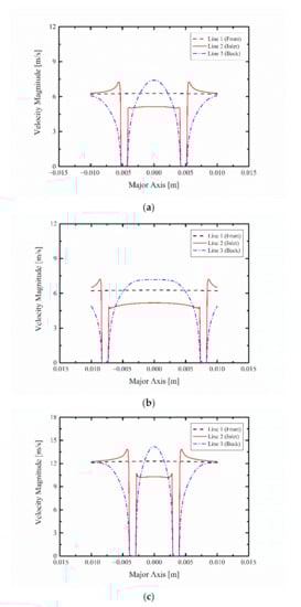

Figure 8.
Velocity distribution around the sampling probe according to free-stream velocity: (a) 5 m/s free-stream, circular inlet; (b) 5 m/s free-stream, ellipsoidal inlet; (c) 10 m/s free-stream, circular inlet; (d) 10 m/s free-stream, ellipsoidal inlet; (e) 15 m/s free-stream, circular inlet; and (f) 15 m/s free-stream, ellipsoidal inlet.
Figure 9 shows the aspiration ratio of the circular and ellipsoidal sampling probes at flow velocities of 5, 10, and 15 m/s. To compare the two inlet shapes, 31,000 particles were uniformly injected at the inlet of the flow field. The aspiration ratio tended to exceed 1 as the flow velocity and particle size increase; in all cases, the aspiration ratio of the ellipsoidal inlet was closer to 1 than that of the circular inlet. This result implies that isokinetic sampling of aerosols in the air is possible when an ellipsoidal nozzle is used. Figure 9a shows the aspiration ratio when the flow velocity is 5 m/s, where the mean aspiration ratios of the circular and ellipsoidal inlets have a 4.1% relative difference with respect to a ratio of 1. The slope of the aspiration ratio increases gradually for all flow-velocity conditions; the ellipsoidal inlet guarantees isokinetic sampling with a 1.0% error rate for particles of PM10 or below, while the circular inlet had a 3.0% error rate, confirming that super-isokinetic sampling occurs as the particle size increases. Figure 9b shows the aspiration ratios when the flow velocity is 10 m/s; the mean aspiration ratios of both inlets have a 2.3% relative difference with respect to a ratio of 1. The ellipsoidal inlet showed isokinetic sampling with a 1.8% error rate for particles with PM10 or below, while the circular inlet had a 2.6% error rate. Figure 9c shows the aspiration ratios of both inlets for a flow velocity of 15 m/s; the mean aspiration ratios differ by 2.0% relatively. The ellipsoidal inlet demonstrated a 1.0% error in isokinetic sampling for the particles below PM10, while the circular inlet exhibited a 1.2% error. The relative difference between the two inlet types decreased as the free-stream velocity increased. Considering all cases, the ellipsoidal and circular inlets had an average difference of 2.8% in terms of the aspiration ratio. Although the circular inlet achieves uniform sampling in the radial direction, the ellipsoidal inlet can correct the aspiration ratio to a certain extent owing to irregular sampling arising from the difference in length in the major-axis direction and radial direction, allowing for the sampling of particles at a similar as the circular inlet.

Figure 9.
Comparison of aspiration ratio according to inlet type of the sampling probe: (a) 5 m/s, (b) 10 m/s, and (c) 15 m/s.
Figure 10 shows a graph plotting the aspiration ratio according to turbulence intensity when the free-stream velocity is 5 m/s for each inlet shape of the sampling probe. The turbulence intensity at the inlet must be specified when setting the boundary conditions in FLUENT. Turbulence intensity is defined as the ratio of the root mean square of velocity changes with respect to mean velocity; in general, a turbulence intensity of 1% or lower is considered low, while an intensity of 10% or higher is considered high [23]. A fast flow inside an inlet with high turbulence generally has a turbulence intensity of 5–20%. Also, the turbulence intensity of a fully developed pipe flow can be calculated using Equation (11) [24].

Figure 10.
Comparison of aspiration ratio according to turbulence intensity: (a) circular inlet and (b) ellipsoidal inlet.
Here, is the Reynolds number based on the pipe hydraulic diameter . The flow-velocity condition used in this study (i.e., 5–15 m/s) corresponds to a turbulence with a Reynolds number of 34,000–102,000 and turbulence intensities of 3.8–4.3%, as calculated using Equation (6).
Figure 10a,b show the aspiration ratios of the circular and ellipsoidal inlets when the turbulence intensity is 5–15%, respectively. The effect on the aspiration ratio was insignificant in the area where the particle size was ≤15 μm and the Stokes number was <1 when the turbulence intensity was 5–15%, which is higher than the actual condition; super-isokinetic sampling tended to occur in the area containing particles of 20 μm or larger. Hence, at higher turbulence intensities, super-isokinetic sampling into the sampling probe may occur owing to the interaction between the particles and turbulent eddy. The Stokes number is a dimensionless number related to the behavior of particles in a fluid and is expressed by Equation (12). When the Stokes number is less than unity, the flow direction changes when encountering an obstacle, and particles move along the streamline. When the Stokes number is greater than unity, the influence of particle inertia increases, and the particle moves in the tangential direction of the streamline [25].
Here, is the relaxation time, is the average flow rate passing through the nozzle, is the diameter of the nozzle, is the density of particles, is the diameter of the particles, is the Cunningham slip correction factor, and is the viscosity coefficient of air. In the range of 1~15 m, the Stokes number is unity at most, and there is no difference in the aspiration ratio depending on the turbulence intensity. However, in the range of 20~50 μm, the Stokes number exceeds unity, and it was confirmed that super-isokinetic sampling is performed as the particle size and turbulence intensity increase. However, since the difference in the aspiration ratio is 1.1%, which corresponds to a turbulence intensity of 5–15%, the effect of turbulence intensity on the aspiration ratio is insignificant.
4. Conclusions
This study examined the effect of the inlet shape of an isokinetic sampler on the aspiration ratio. The aspiration ratio was analyzed at free-stream velocities of 5, 10, and 15 m/s by modeling a circular inlet with identical lengths in the radial direction and an ellipsoidal inlet with a rectangular shape in the middle along the major-axis and a semi-circle shape on both ends. We performed a simulation by setting the suction flow rate of the sampling probe to 16.7 L/min, the pressure to atmospheric pressure, and temperature to 300 K in order to isolate the effect of the inlet shape on the aspiration ratio. The uniformity was analyzed to determine if the flow was fully developed, and both the circular and ellipsoidal inlets exhibited a uniformity of at least 0.92 in all flow-velocity ranges of the free stream. Furthermore, an analysis of the velocity magnitude near the inlet tip of the sampling probe indicated that the velocity boundary layer inside the sampling probe formed earlier in the ellipsoidal inlet than in the circular inlet at a flow velocity of 5 m/s; moreover, the velocity of the latter was 0.92% closer to that of the free-stream velocity than that of the former when the flow velocity was 15 m/s. The aspiration ratio according to inlet shape increased as the particle size and flow velocity increased; the ellipsoidal inlet was 1.8% to 3.7% more effective at isokinetic sampling than the circular inlet. This result indicates that the ellipsoidal nozzle is capable of isokinetic sampling, and its economic feasibility lies in the ability to adjust the length of the major axis. This is an advantage over the circular nozzle, which requires inlets of different diameters depending on the measurement environment. Lastly, the effect of turbulence intensity on the aspiration ratio was examined by adjusting the turbulence intensity of the free stream from 5 to 15%; an insignificant effect was observed for both inlets. In future studies, further analyses are required for the cases of an ellipsoidal nozzle with an area gradually expanding past the sampling inlet plane, and when the inlet tip forms an acute rather than orthogonal angle with the flow. Moreover, the aspiration ratio must be analyzed at various flow velocities to account for aerosol sampling by devices installed on fast-moving vehicles such as automobiles or unmanned air vehicles.
Author Contributions
Conceptualization, J.-H.N.; Methodology, M.-C.C. and J.-H.Y.; Software, J.-H.Y.; Validation, M.-C.C.; Formal analysis, M.-C.C.; Investigation, M.-C.C.; Resources, J.-H.Y.; Data curation, M.-C.C.; Writing—original draft preparation, M.-C.C.; Writing—review and editing, D.-S.K. and J.-H.N.; Visualization, M.-C.C.; Supervision, J.-H.N.; Project administration, D.-S.K. and J.-H.N.; Funding acquisition, J.-H.N. All authors have read and agreed to the published version of the manuscript.
Funding
This work was supported by the Korea Institute of Energy Technology Evaluation and Planning (KETEP) and the Ministry of Trade, Industry & Energy (MOTIE) of the Republic of Korea (No. 20181110200170).
Institutional Review Board Statement
Not applicable.
Informed Consent Statement
Not applicable.
Data Availability Statement
Not applicable.
Conflicts of Interest
The authors declare no conflict of interest.
References
- Kim, B.-U.; Kim, O.; Kim, H.; Kim, S. Influence of fossil-fuel power plant emissions on the surface fine particulate matter in the Seoul Capital Area, South Korea. J. Air Waste Manag. Assoc. 2016, 66, 863–873. [Google Scholar] [CrossRef] [PubMed]
- Miller, F.J.; Gardner, D.E.; Graham, J.A.; Lee, R.E.; Wilson, W.E.; Bachmann, J.D. Size Considerations for Establishing a Standard for Inhalable Particles. J. Air Pollut. Control Assoc. 1979, 29, 610–615. [Google Scholar] [CrossRef]
- Manisalidis, I.; Stavropoulou, E.; Stavropoulos, A.; Bezirtzoglou, E. Environmental and Health Impacts of Air Pollution: A Review. Front. Public Health 2020, 8, 14. [Google Scholar] [CrossRef] [PubMed]
- Heo, N.-G.; Lim, J.-H.; Lee, J.-W.; Lee, J.-S.; Yook, S.-J.; Ahn, K.-H. Development of a Sampling Probe for Representative Sampling of PM at Freestream Velocities in the Range from 0 to 300 km h−1. J. Atmos. Ocean. Technol. 2018, 35, 727–738. [Google Scholar] [CrossRef]
- Kanemoto, K.; Moran, D.; Lenzen, M.; Geschke, A. International trade undermines national emission reduction targets: New evidence from air pollution. Glob. Environ. Chang. 2014, 24, 52–59. [Google Scholar] [CrossRef]
- Shin, D.; Woo, C.G.; Hong, K.-J.; Kim, H.-J.; Kim, Y.-J.; Han, B.; Hwang, J.; Lee, G.-Y.; Chun, S.-N. Continuous measurement of PM10 and PM2.5 concentration in coal-fired power plant stacks using a newly developed diluter and optical particle counter. Fuel 2020, 269, 117445. [Google Scholar] [CrossRef]
- Moteki, N.; Kondo, Y.; Nakayama, T.; Kita, K.; Sahu, L.K.; Ishigai, T.; Kinase, T.; Matsumi, Y. Radiative transfer modeling of filter-based measurements of light absorption by particles: Importance of particle size dependent penetration depth. J. Aerosol Sci. 2010, 41, 401–412. [Google Scholar] [CrossRef]
- Jaworek, A.; Marchewicz, A.; Krupa, A.; Sobczyk, A.T.; Czech, T.; Antes, T.; Kurz, M.; Szudyga, M.; Rożnowski, W. Dust particles precipitation in AC/DC electrostatic precipitator. J. Phys. Conf. Ser. 2015, 646, 012031. [Google Scholar] [CrossRef]
- Hemeon, W.C.L.; Haines, G.F. The Magnitude of Errors in Stack Dust Sampling. Air Repair 1954, 4, 159–164. [Google Scholar] [CrossRef][Green Version]
- Baron, P. Generation and Behavior of Airborne Particles (Aerosols). Available online: https://www.cdc.gov/niosh/topics/aerosols/pdfs/Aerosol_101.pdf (accessed on 30 August 2022).
- Wilcox, J.D. Isokinetic Flow and Sampling. J. Air Pollut. Control Assoc. 1956, 5, 226–245. [Google Scholar] [CrossRef]
- Baron, P.A.; Chen, C.-C.; Hemenway, D.R.; O’Shaughnessy, P. Nonuniform Air Flow in Inlets: The Effect on Filter Deposits in the Fiber Sampling Cassette. Am. Ind. Hyg. Assoc. J. 1994, 55, 722–732. [Google Scholar] [CrossRef] [PubMed]
- Lim, J.-H.; Park, S.-H.; Yook, S.-J.; Ahn, K.-H. Aspiration ratio of a double-shrouded probe under low pressure conditions in troposphere. Aerosol Sci. Technol. 2020, 54, 1323–1334. [Google Scholar] [CrossRef]
- Dunnett, S.J.; Ingham, D.B. An Empirical Model for the Aspiration Efficiencies of Blunt Aerosol Samplers Orientated at an Angle to the Oncoming Flow. Aerosol Sci. Technol. 1988, 8, 245–264. [Google Scholar] [CrossRef]
- Kalatoor, S.; Grinshpun, S.A.; Willeke, K.; Baron, P. New aerosol sampler with low wind sensitivity and good filter collection uniformity. Atmos. Environ. 1995, 29, 1105–1112. [Google Scholar] [CrossRef]
- Rader, D.J.; Marple, V.A. A Study of the Effects of Anisokinetic Sampling. Aerosol Sci. Technol. 1988, 8, 283–299. [Google Scholar] [CrossRef]
- Badzioch, S. Collection of gas-borne dust particles by means of an aspirated sampling nozzle. Br. J. Appl. Phys. 1959, 10, 26–32. [Google Scholar] [CrossRef]
- McFarland, A.R.; Ortiz, C.A.; Moore, M.E.; Otte, R.E.D., Jr.; Somasundaram, S. A shrouded aerosol sampling probe. Environ. Sci. Technol. 1989, 23, 1487–1492. [Google Scholar] [CrossRef]
- Ram, M.; Cain, S.A.; Taulbee, D.B. Design of a shrouded probe for airborne aerosol sampling in a high velocity airstream. J. Aerosol Sci. 1995, 26, 945–962. [Google Scholar] [CrossRef]
- Gong, H.; Anand, N.K.; McFarland, A.R. Numerical Prediction of the Performance of a Shrouded Probe Sampling in Turbulent Flow. Aerosol Sci. Technol. 1993, 19, 294–304. [Google Scholar] [CrossRef]
- ANSYS. ANSYS Theory Reference; ANSYS Inc.: Canonsburg, PA, USA, 2020. [Google Scholar]
- Hinds, W. Aerosol Technology: Properties, Behavior, and Measurement of Airborne Particles; John Wiley & Sons: New York, NY, USA, 1999. [Google Scholar]
- ANSYS. ANSYS FLUENT 12.0. Theory Guide; ANSYS Inc.: Canonsburg, PA, USA, 2009. [Google Scholar]
- CFD Online. Turbulence Intensity. Available online: https://www.cfd-online.com/Wiki/Turbulence_intensity (accessed on 30 August 2022).
- Marjamäki, M.; Keskinen, J.; Chen, D.-R.; Pui, D.Y.H. Performance Evaluation of the Electrical Low-Pressure Impactor (ELPI). J. Aerosol Sci. 2000, 31, 249–261. [Google Scholar] [CrossRef]
Publisher’s Note: MDPI stays neutral with regard to jurisdictional claims in published maps and institutional affiliations. |
© 2022 by the authors. Licensee MDPI, Basel, Switzerland. This article is an open access article distributed under the terms and conditions of the Creative Commons Attribution (CC BY) license (https://creativecommons.org/licenses/by/4.0/).