Robustness, Stability, and Fidelity of Explanations for a Deep Skin Cancer Classification Model

Abstract

Skin cancer is one of the most prevalent of all cancers. Because of its being widespread and externally observable, there is a potential that machine learning models integrated into artificial intelligence systems will allow self-screening and automatic analysis in the future. Especially, the recent success of various deep machine learning models shows promise that, in the future, patients could self-analyse their external signs of skin cancer by uploading pictures of these signs to an artificial intelligence system, which runs such a deep learning model and returns the classification results. However, both patients and dermatologists, who might use such a system to aid their work, need to know why the system has made a particular decision. Recently, several explanation techniques for the deep learning algorithm’s decision-making process have been introduced. This study compares two popular local explanation techniques (integrated gradients and local model-agnostic explanations) for image data on top of a well-performing (80% accuracy) deep learning algorithm trained on the HAM10000 dataset, a large public collection of dermatoscopic images. Our results show that both methods have full local fidelity. However, the integrated gradients explanations perform better with regard to quantitative evaluation metrics (stability and robustness), while the model-agnostic method seem to provide more intuitive explanations. We conclude that there is still a long way before such automatic systems can be used reliably in practice.

1. Introduction

Skin cancer is one of the most prevalent cancer types [1,2]. The Center for Disease Control and Prevention estimates that there are 44 million visits to dermatologists every year, with skin lesions being one of the primary reasons for these visits [3]. Automating some of the tasks dermatologists work with, would not only bring a relief to the rising workload dermatologists struggle with but also make regular assessments easier and more affordable to a large number of patients. In recent years, advances in computer vision techniques and deep neural networks have yielded models that can automatically classify skin cancer. More specifically, the ability of convolutional neural networks (CNNs) to learn features have been noted also in the medical image analysis domain [4], and the dermatology subfield [1,2,5,6]. As a whole, CNNs have become a widely used and “state-of-art” technique when developing algorithms for medical image classification (including dermatology) tasks.

To our knowledge, in 2019, Brinker et al. [7] reported, for the first time, an on par skin cancer classification performance of CNN with dermatologists. Since then, scholars have increasingly published studies of automatic skin lesion classification models outperforming human domain experts/ dermatologists [8]. In fact, a recent survey by Haggenmüller et al. [9] reports that in all their reviewed works, AI showed superior or at least equivalent performance compared with clinicians. However, one of the main disadvantages of CNNs with their many layers and weights is that they are opaque. This means that it is unclear why a CNN arrived at a certain decision, making it difficult to trust the models. Thus, before these models can be integrated into clinical practice, the interpretability gap needs to be filled [10].

As explained by Selvaraju et al. [11], there are three main reasons why interpretability matters, and these reasons mostly related to how well the AI system is performing in comparison to human decision-makers: First, if the human decision-maker is performing better than the AI system, interpretability is needed mostly as a debugging function (i.e., for establishing the reasons why and where the AI is not performing as expected). As summarized by Maron et al. [12], CNNs can suffer from a variety of flaws, and it is important to detect these flaws. Secondly, if the human and the AI are more or less on par, the interpretability need mainly arises to convince users to have confidence and trust in the AI (e.g., by showing that the human domain expert would decide exactly as the AI system). Thirdly, if the AI outperforms the human domain expert, the interpretability can show or teach humans to become better (e.g., by highlighting the most important features one should pay attention to or providing general rules).

In this study, we are interested in all three reasons. For our experiments, we use the well-known HAM10000 data [13], an established public dataset for benchmarking and training of dermatology tasks. This dataset contains more than 10,000 dermascopic images spread between seven different types of skin lesions. According to a 2020 paper by Tschandl et al. [8], human domain expert classification performance for this dataset is about 64%, while current CNNs clearly outperform the human experts. This means that the interpretability of such an AI system/CNN model might actually teach humans tricks or rules helping them to make better decisions/classifications of skin lesions. However, we also want to make sure that the reasons why these models make particular decisions, make sense (e.g., that no unreasonable parts of the skin lesion images, such as hair, are utilized for the classification), and that humans (both domain experts as well as patients) have more arguments and justification to trust and confide in such AI systems. As pointed out by Gaube et al. [14], AI systems will only be able to provide real clinical benefit if the physicians using them can balance trust and skepticism. On the one hand, physicians, who do not trust the technology, will not use it. On the other hand, blind trust in the technology can lead to medical error. Explainable AI promises a solution to these problems: provide explanations to increase trust and informed decision-making; and give reasons/a glass-box for the AI’s decisions, instead of condoning black-box decisions.

More specifically, explainable AI (XAI), sometimes also called interpretable machine learning (IML), is an emerging research direction concerned with helping the user or developer of complex machine learning models to understand the model’s underlying decision process, and why these models behave the way they do [15,16,17,18,19]. XAI/IML techniques can be divided into global and local ones. Global interpretation methods provide explanations for the whole dataset, while the latter provide explanations for specific instances. Because we rely on the automatic feature extraction by CNNs, we cannot use intrinsically interpretable classification models that give us model-specific global explanations (such as random forest, decision tree, or logistic regression). Moreover, the local ones are more useful for our case, where we want to provide the patient with classification results and explanations for his/her specific lesion images. Thus, to address the dermatology AI interpretability issue, we compare two currently popular local XAI/IML techniques for images; one gradient- and one perturbation-based method:

• Integrated gradients [20], which calculate feature attributions to the prediction by accumulating gradients along a path from a baseline instance to the specific instance of interest.
• Local interpretable model-agnostic explanations [21], which build an interpretable surrogate model around the decision space of the CNN model’s prediction in the local neighbourhood of the specific instance of interest.

To compare the explanations quantitatively, we compute their performance with regard to three metrics: robustness, stability, and fidelity. Moreover, we provide the visual explanations for the “most interesting” [22,23] explanation cases: those, which the CNN classifier classifies correctly and incorrectly with the highest probability.

As pointed out in a recent review of explanation techniques for the medical domain [19], new XAI/IML are introduced constantly, but metrics and comparison studies are needed to assess and validate these techniques. To address this research gap, our main contribution is the qualitative and quantitative comparison of two popular explanation techniques for a deep CNN model. Although some skin cancer classification studies used visualizations to explain a few local classifications of their CNN models (e.g., [2,5,24]), to our knowledge, no study exists that quantitatively compares such explanations through metrics. Thus, our focus lies on the quality of the XAI/IML techniques that create such visualizations. In comparison to related work, we quantitatively and qualitatively compare the outcomes of different explanation techniques for the same model and the same classifications, while related work only showed a few local explanations/visualizations of randomly (i.e., with no reported rule) picked instances.

The remainder of this paper is structured as follows. Section 2 describes the HAM1000 data and used methods. More specifically, we explicate the deep learning models’ performance–interpretability trade-off, and how XAI/IML techniques work to address this trade-off. We also depict the quantitative metrics that we used to compare the explanation techniques. Section 3 presents the experimental results. Section 4 concludes our analysis, and discusses limitations and future work.

2. Material and Methods

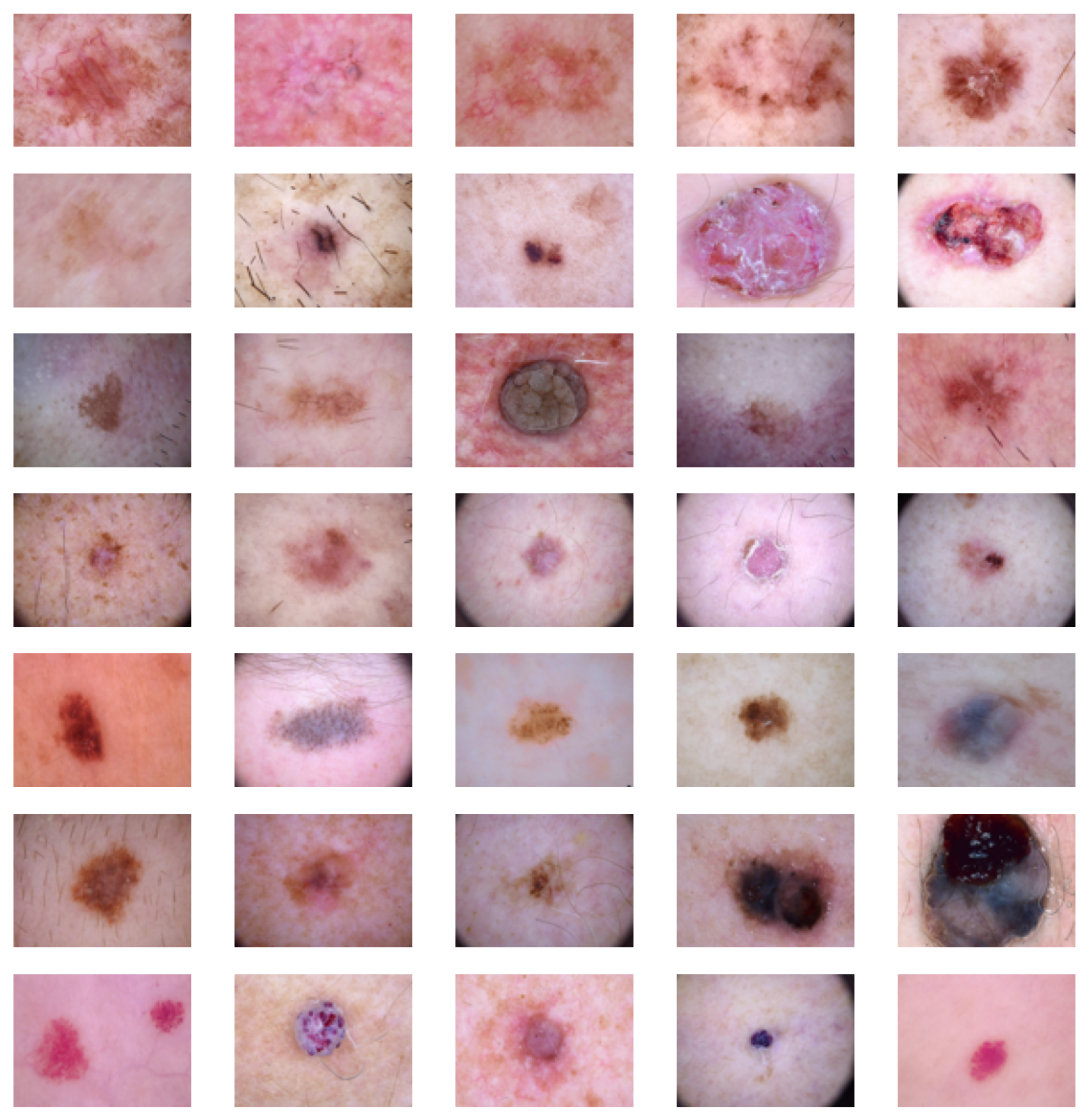
2.1. Data

We used the HAM10000 dataset, a large public collection of dermatoscopic images, for our experiments. This dataset can be downloaded from the International Skin Imaging Collaboration (ISIC). (See https://www.isic-archive.com/, accessed on 10 August 2022). It consists of 10,050 dermoscopic images belonging to seven different classes. More specifically, 6705 images belong to the melanocytic nevi (nv) class, 1113 belong to the melanoma (mel) class, 1099 belong to the benign keratosis-like lesions (bkl) class, 514 belong to the basal cell carcinoma (bcc) class, 327 belong to the actinic keratoses (akiec) class, 142 belong to the vascular lesions (vasc) class, and 115 images belong to the dermatofibroma (df) class. Figure 1 shows five randomly picked examples of each of these classes.

These 10,015 dermoscopic images were collected over a time period of 20 years from the department of dermatology at the Medical University of Viena, Austria, and the skin cancer practice of Cliff Rosendahl in Queensland, Australia (see [13] for a detailed description of this dataset). Since then, they have become a widely used dataset for dermatology benchmarking and training.

As mentioned in the introduction, human domain expert classification performance for this dataset is about 64% [8], while current ML models mostly outperform the human experts in classification accuracy. In a recent article, Cassidy et al. [1] compared several popular deep learning architectures for this dataset and reported the best performance for EfficientNetB0 with an accuracy of 62.1% (see Table 13 in [1]). Eestava et al. [2] reported a higher accuracy (72.1%), but they used external data to augment the dataset and the 72.1% is only for the classification into three types (i.e., benign, malignant, and neoplastic). Tschandl et al. [8] used a 34-layer residual network and achieved an accuracy of 80.3% on the classification into the seven classes in the data (i.e., askiec, bcc, bkl, df, mel, nv, and vasc). This is similar to the accuracy we achieve with a significantly simpler model (see Section 3), and a result that outperforms human expert classifications and that ranks in the top quartile of all ML models developed for the HAM10000 dataset [8].

A full overview of related work using the ISIC data and skin cancer classification models is out of scope for this article. Moreover, it would shift its focus which lies on the explanations of the classifications. A plethora of articles reviewing skin cancer classification models exist already. Thus, we refer the interested reader to one these overviews. For example, Table 1 by Cassidy et al. [1] provides a very recent overview of research papers using ISIC data for skin cancer classification, Höhn et al. [25] survey approaches of integrating patient data into skin cancer CNN classification models, Gulzar and Khan [26] compare studies that use U-Net and attention-based methods for skin lesion image segmentation, and the study by Thurnhofer-Hemsi and Domínguez [6] includes a recent summary of papers using specifically the HAM10000 dataset for deep learning skin cancer classification models. In addition, articles have been published that highlight the increasing performance with transfer learning approaches [27], the significance of specific techniques for the multi-class classification [28], and the usefulness of CNN ensemble techniques [29].

2.2. Methods

All experiments were performed in Python 3.9.7, using tensorflow version 2.8.1. Explanations were created using the open-source packages alibi-explain [30] and LIME [21].

2.2.1. Deep Learning

Deep learning networks are based on artificial neural networks, which are composed of neurons organized in layers [31]. In comparison to traditional or “shallow” neural networks, deep networks use multiple layers to progressively extract higher-level features from the raw input [32,33]. This automatic feature extraction is one of the main advantages of deep learning since not everything needs to be programmed explicitly [34]. It is also one the reasons why deep learning networks have shown exceptional performance, especially in (medical) image analysis, where manual feature engineering is a time-consuming and error-prone process [4]. However, this advantage comes with the trade-off that deep learning models, with their many kinds of processing layers and multitudes of weights, are also reckoned to be one of the least interpretable machine learning models [18].

Deep learning models can be categorized into multi-layer neural networks that take non-structured data as input, and CNNs that take structured data as input. For (medical) image analysis, CNNs are the most common choice, because of the structural characteristic of images, that is, the structural information among neighbouring pixels or voxels is another source of information [4,33,35]. The core building blocks of a CNN are convolutional layers (giving CNNs their name), pooling layers, and fully connected layers [4,36]. The convolutional layers produce feature maps by applying convolutional operations to the input. More specifically, the units of the convolution layer l compute their activations ${\mathit{A}}_j^{\left(l\right)}$ based only on a spatially contiguous subset of units in the feature maps ${\mathit{A}}_j^{(l-1)}$ of the preceding layer $l-1$ by convolving the kernels $k_{ij}^{\left(l\right)}$ as follows:

$${\mathit{A}}_j^{\left(l\right)}=f(\sum _{i=1}^{M^{(l-1)}}{\mathit{A}}_j^{(l-1)}\ast k_{ij}^{\left(l\right)}+b_j^{\left(l\right)})$$

(1)

with $M^{(l-1)}$ being the number of feature maps in the $l-1$ layer, ∗ being a convolution operator, $b_j^{\left(l\right)}$ being a bias parameter, and $f(·)$ being a non-linear activation function. Pooling layers can be added to down-sample the feature maps of the preceding convolution layer and, through that, “squeeze” the amount of information that is passed on to the next layer. Fully connected layers are the ones solving the final classification problem with the data they have from the previous layer [31].

Table 1. Summary and overall architecture of the CNN model used in this study.

Layer	Type	Output Shape	Number of Parameters
conv2d	Conv2D	(None, 200, 150, 32)	896
conv2d_1	Conv2D	(None, 200, 150, 32)	9248
max_pooling2d	Max_Pooling2D	(None, 100, 75, 32)	0
dropout	Dropout	(None, 100, 75, 32)	0
conv2d_2	Conv2D	(None, 100, 75, 64)	18,496
conv2d_3	Conv2D	(None, 100, 75, 64)	36,928
max_pooling2d_1	Max_Pooling2D	(None, 50, 37, 64)	0
dropout_1	Dropout	(None, 50, 37, 64)	0
flatten	Flatten	(None, 118,400)	0
dense	Dense	(None, 128)	15,155,328
dropout_2	Dropout	(None, 128)	0
dense_1	Dense	(None, 7)	903

reports the summary and overall architecture of the CNN used in this study. We built our CNN with the Keras Sequential API and trained it by using 150 epochs, a batch size of 10, the Adam optimizer with categorical cross-entropy as the loss function, and 0.0001 as the learning rate. As the non-linear activation function (i.e., $f(·)$ in Equation (1)) we chose the rectified linear unit (ReLU) activation function.

2.2.2. Explanation Techniques

Explainable artificial intelligence (XAI), sometimes also called interpretable machine learning (IML), is a new research area. Several surveys about this topic have been published recently [15,16,17,19] underlining its topicality. Explainability is presented either as inherent characteristic of an algorithm or as an approximation by other methods [37]. The latter is highly important for methods that have until recently been labeled as “black-box”, such as artificial neural networks. To explain their predictions, however, numerous methods exist today [37,38]. Generally, predictive modelling implies a trade-off: the reason for the prediction versus how accurate it is. This means that the performance of complex models with non-linear combinations of inputs usually is better, but such models are harder or even impossible to understand. As pointed out before, deep learning models are typically on the extreme ends: they usually outperform all other machine learning techniques with regard to predictive accuracy (especially in image analysis tasks), but they are also the least interpretable. XAI/IML refer to approaches attempting to make machine learning models more explainable.

The need for interpretability arises from an incompleteness in problem formalization [39], which means that for certain problems or tasks it is not enough to obtain the prediction (the what). The model must also explain how it came to the prediction (the why), because a correct prediction only partially solves the original problem. The following reasons drive the demand for interpretability and explanations [40]: compliance and trust related to uptake of health care applications, transparency and reproducibility of the AI decision-making process, and potentially mitigation of bias in health care. The challenge when using AI models as black boxes has resulted in a lack of accountability and trust in the decisions which XAI aims to rectify.

Generally, XAI/IML methods can be categorized into

• Intrinsic versus post hoc;
• Global versus local;
• Model-specific versus model-agnostic;
• Perturbation- or occlusion-based versus gradient-based.

Intrinsic XAI/IML methods refer to techniques that are explainable by themselves (e.g., due to their simple structure, such as linear regression models), while post hoc methods explain the model’s logic in retrospect after it was trained. Moreover, one distinguishes between local and global explanations. Although modular global explanations provide interpretation for the model as a whole, approaching it holistically, a local explanation provides interpretation for a specific observation (such as one particular image). Furthermore, an explanation technique can be model-specific if it depends on (parts of) its model, or model-agnostic, if it can be applied to any model. Occlusion- or perturbation-based methods manipulate parts of the image to generate explanations, while gradient-based methods compute the gradient of the prediction (or classification score) with respect to the input features.

Another way to categorize XAI/IML methods is the manner in which they provide explanations. They can be either based on examples (e.g., [41,42,43]), counterfactuals (e.g., [44]), hidden semantics (e.g., [45]), rules (e.g., [46,47,48]), or features/attributions/saliency (e.g., [49,50,51,52]). The most common explanation for classification models are the latter, that is, feature importances [22]. Feature importances rely on feature scoring and ranking to quantify and improve the understandability of a model, and thereby explain its behaviour [53]. If the model is trained on images (i.e., features refer to (super-)pixels of the images), one also speaks about “saliency maps” or “pixel attribution” explanation methods. Saliency of features to rank their explanatory power is applicable in both feature selection and as a post hoc explainability approach [16,54].

Both XAI/IML methods we use in this work, that is, integrated gradients by Sundararajan et al. [20] and local model-agnostic explanations (LIME) by Ribeiro et al. [21], provide explanations as feature importances. Moreover, they are both post hoc methods that are applied after model training. However, LIME is model-agnostic and can be applied to any model, while integrated gradients can only be applied to any differentiable model. Moreover, LIME is perturbation-based and integrated gradients is gradient-based.

For neural networks, one measure of feature importance/saliency is the input sensitivity, that is, the partial derivative of the network’s output with respect to its input. For shallow networks, feature assessment originating from this idea was proposed by Dimopoulos et al. [55]. Use of a partial derivative method was rediscovered within the context of deep neural networks by Simonyan et al. [56], where it was used to generate an image-specific saliency map for visual interpretation of a CNN classifier. However, these early gradient-based techniques suffer from the saturation problem [20,57]. Meaning that the more a model learns the relationship between the range of an individual feature and the prediction, the gradient for this feature will become increasingly small and even go to zero. To solve this saturation problem, the integrated gradients technique by Sundararajan et al. [20] accumulates gradients along a path from a baseline instance $x^{\prime }$ to the specific instance of interest. The integrated gradient for a particular instance x is defined as

$$(x_i-x_i^{\prime })\times {\int }_{\alpha =0}^1\frac{\delta F(x^{\prime }+\alpha \times (x-x^{\prime }))}{\delta x_i}d\alpha$$

(2)

where i is a feature (pixel), and $\frac{\delta F\left(x\right)}{\delta x_i}$ is the gradient of $F\left(x\right)$ along the ith feature.

LIME is perturbation-based and does not need access to any model internals. It works for tabular, text, and image data. It takes the instance x for which the prediction should be explained and permutes depending on the data type, either its feature values (for tabular and text data) or its superpixels (i.e., interconnected pixels with similar colour) for image data. These permuted instances are then weighted by their distance to x, the model f is used to predict the permuted instances, and a new surrogate model g is trained. Optimization is used to find a local surrogate model with low complexity but high agreement with the prediction of the original model. In short, LIME is defined as follows:

$$\xi =\underset{g\in G}{arg\; min}\mathcal{L}(f,g,{\pi }_x)+\mathsf{\Omega }\left(g\right),$$

(3)

where ${\pi }_x$ is the proximity measure to define locality around x, and $\mathsf{\Omega }\left(g\right)$ is the complexity of g.

2.2.3. Metrics

There is no general consensus among scholars on how the quality and reliability of explanation techniques should be assessed [58]. Generally, one can distinguish between human-centred qualitative evaluations and more objective metrics [58]. In this paper, we provide qualitative visual explanations only for the “most interesting cases” [22], and focus the main validation assessment to the latter. More precisely, we use three objective quantitative evaluation metrics: robustness, stability, and fidelity.

First, we measure the robustness of the explanation techniques using the Lipschitz indicator proposed by Alvarez-Melis and Jaakkola [59]. This Lipschitz indicator gives the persistence of an explanation method to withstand small perturbations of the input that do not change the prediction of the model. More precisely, Alvarez-Melis and Jaakkola proposed to artificially perturb the features of each object $x_i\in X$, so that ${\mathcal{N}}_{ϵ}\left(x_i\right)=\left|\right|x_i-x_j\left|\right|\le ϵ,$ and then computing the quantity

$$L_X\left(x_i\right)=\underset{x_j\in {\mathcal{N}}_{ϵ}\left(x_i\right)\le ϵ}{arg\; max}\frac{\left|\right|f\left(x_i\right)-f\left(x_j\right)\left|\right|}{\left|\right|x_i-x_j\left|\right|}$$

(4)

to measure whether the explanation technique is robust in a Lipschitz sense. As pointed out in [59], there is no single ideal value for this robustness estimate, because it is highly dataset dependent. However, a smaller value corresponds to more robustness [59]. To measure the robustness of our explanation techniques, we compute the mean and standard deviation of the Lipschitz indicator for all naturally similar instances in the test set (i.e., those test set instances that belong to the same class), so that we do not have perturb any instances artificially.

Second, we measure the stability or identity [60] of the explanation technique by repeating the explanation generation for the same instance and model with the same configuration arguments. If the explanation technique results in different explanations, the technique is not stable. To measure the degree of stability, we simply compute the explanation for each instance in the test set twice with the same configurations and take the percentage of same explanations from all the explanations pairs in the test set. A higher percentage means more stability.

Third, we measure the fidelity. The fidelity metric indicates how closely the surrogate model reflects the real model. By definition, the fidelity of an intrinsically explainable model-specific explanation is always 100%, as it harnesses the original model. However, for model-agnostic explanation techniques, which (such as LIME) are based on local surrogate models, the fidelity is an important objective quality metric. As pointed out by Carvalho et al. [38], an explanation with low fidelity is essentially useless. Similarly as the stability, we report the local fidelity of the explanation technique as percentage for each observation in the test set. Meaning for each observation in the test set, we compute the prediction of the original model and the prediction of the (surrogate) explanation model and report the percentage of agreement.

3. Experimental Results

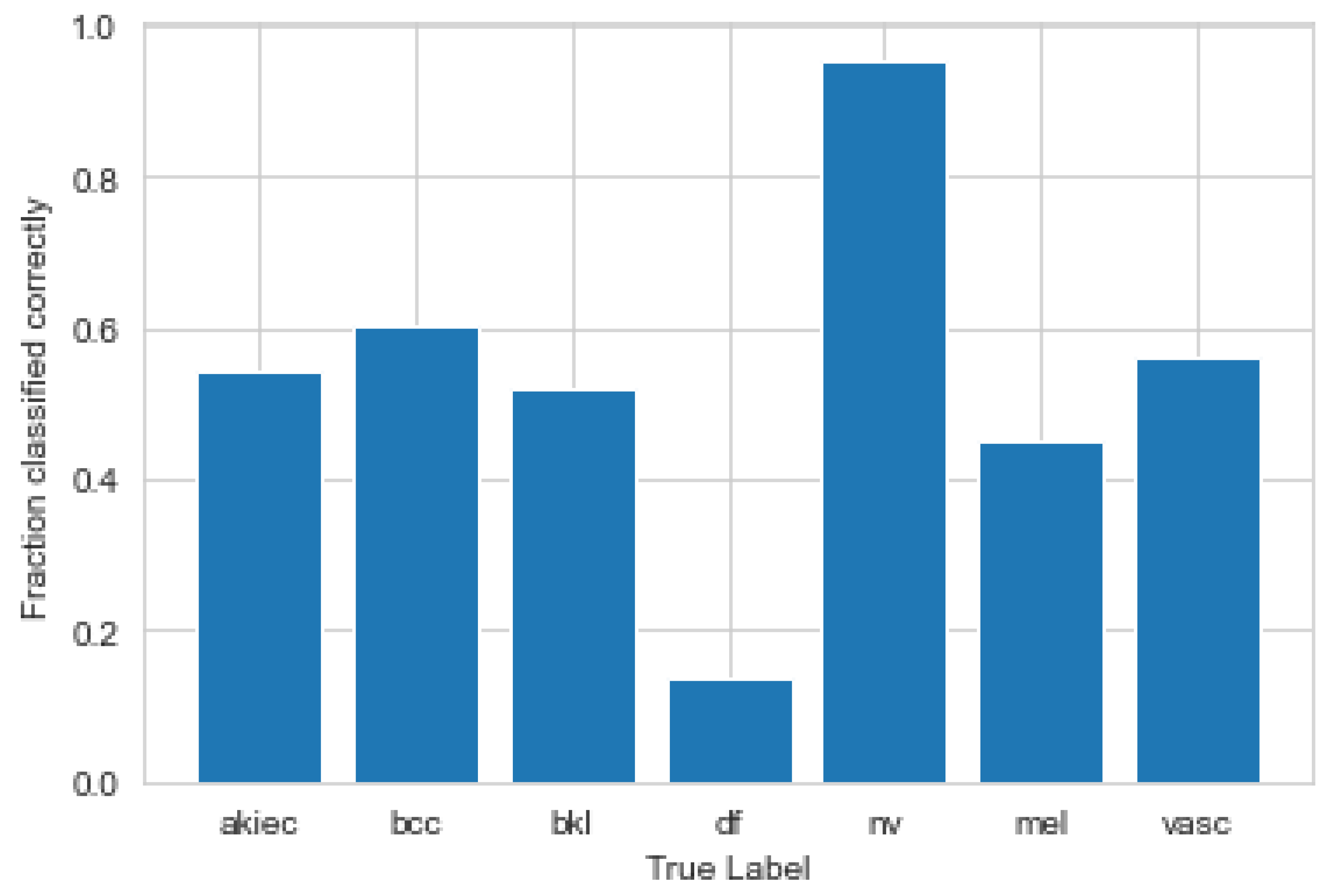
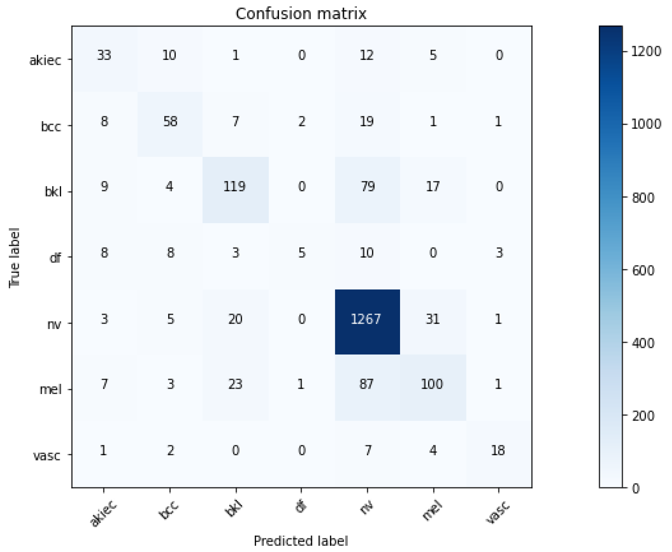
3.1. Convolutional Neural Network

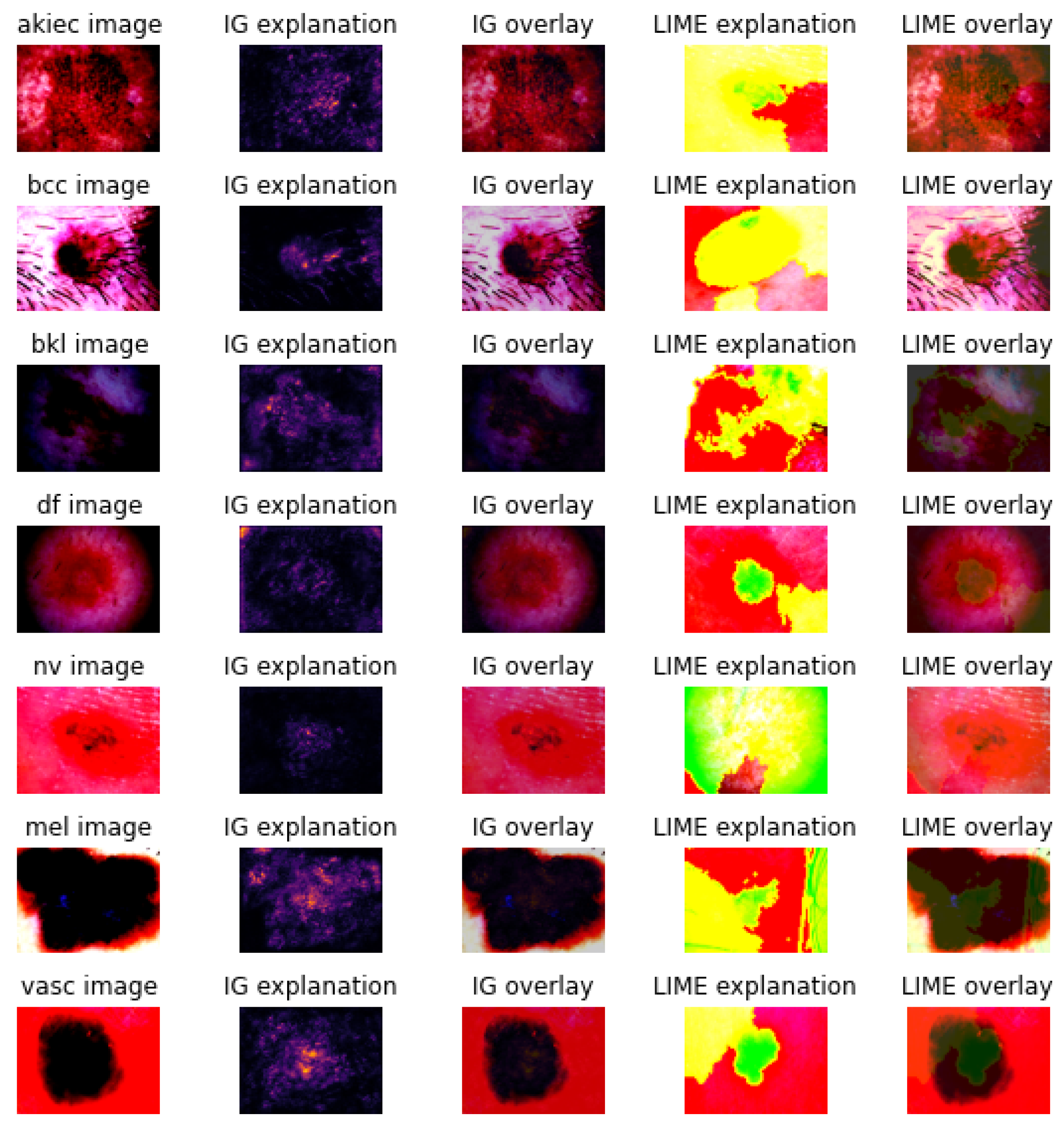
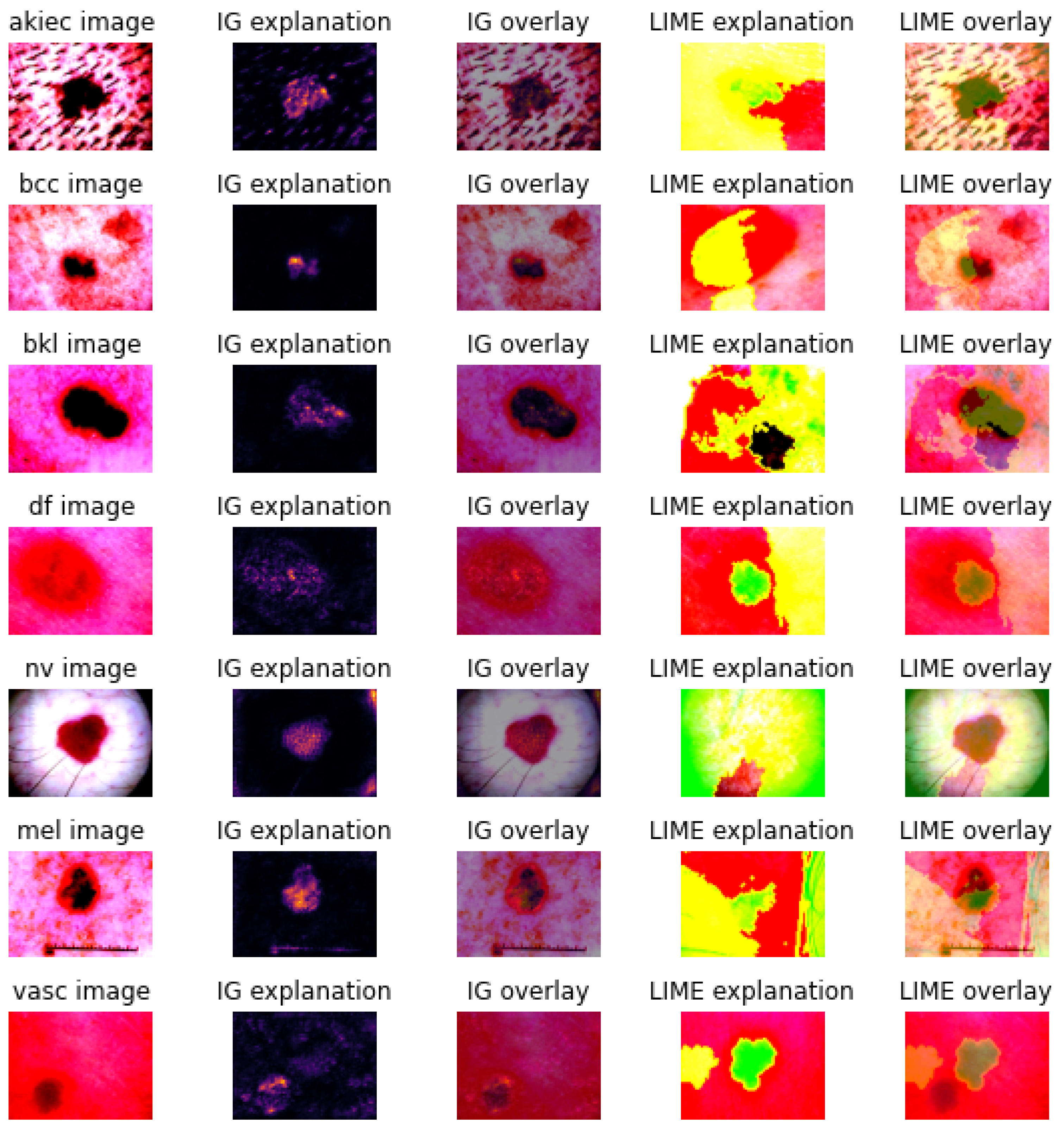
First, the data were divided into a train (80%) and a test (20%) sets. Second, the train set was divided further into a training (90%) and a validation (10%) set. Because of the high imbalance of the classes, we used a stratified split to ensure that the fraction of images from the same class was similar in train and validation sets [61]. To prevent data snooping, only the training and validation set were used during model training, and the test set was kept separately the whole time and used only to test the final the model.

The final model had a performance of 80% accuracy on the test set. Figure 2 shows the confusion matrix of the test set for our final model, and Figure 3 shows the percentage of correct classifications as a bar plot. As expected, performance was best for the melanocytic nevi (nv) class, which had the most images to learn from. It was worst for the actinic keratoses (akiec) class, which had the third least images to learn from, and, thus, is one of the minority classes in the dataset. More training images of the minority classes (i.e., dermatofibroma, vascular lesions, and actinic keratoses) would help the classifier to extract more specific characteristics of these three classes and, thus, improve the overall classification performance.

3.2. Explanations

We computed the feature (pixel) attributions using integrated gradients and LIME on top of the CNN for each image in the test set. Because both explanation techniques provide only local explanations, it is clearly infeasible to show explanations for all the images. Therefore, similarly to Saarela and Jauhiainen [22], we show the explanations for the “most interesting” instances for each class, that is, those images from the test set that the CNN classified correctly and those that the CNN classified incorrectly with the highest probability.

Figure 4 shows the feature (pixel) attributions using the two explanation techniques for those images in the test set that the CNN classified correctly with the highest probability. Figure 5 shows the integrated gradients and LIME explanations for those images, where the CNN did not perform as wanted, that is, those images in the test set that the CNN misclassified with the highest probability. For all classes (except the melanocytic nevi class), the test set images that were misclassified with the highest probability, were classified as belonging to the melanocytic nevi (nv) class. This makes sense as the classifier is clearly biased towards the majority class. The melanocytic nevi test image that was misclassified with the highest probability belonged to the basal cell carcinoma class.

Previous work (see, e.g., [62]) mainly compared feature attributions/maps for ImageNet labels (e.g., cats or dogs). The feature maps learned on the medical images are more challenging to interpret. For example, while it makes sense that a network classifies an animal with sharp ears and whiskers as a cat, there are no such clear rules for skin lesions types. Such approaches commonly use clustering and dimension reduction methods and are applicable to strictly defined domains. For example, Dindorf et al. proposed an explainable pathology independent classifier for spinal posture [63]. The authors used SVM and random forest as the ML classifiers and then applied LIME to explain the prediction of the ML classifier. However, for our data, it seems that the integrated gradients method is able to harness the shape of the lesions. The LIME explanations seem to use more features/pixels to explain, and seem, therefore, somewhat more intuitive.

Most approaches to assurance of safety and reliability of interpretations and as a result their explainability emphasize verification and validation, although the definitions of the terms can vary. The International Medical Devices Regulator Forum (IMDRF) define the terms as follows: Verification—confirmation through provision of objective evidence that specified requirements have been fulfilled; and Validation—confirmation through provision of objective evidence that the requirements for a specific intended use or application have been fulfilled [64]. Explainability is of particularly high value when compliance is required and for applications where predictive performance is not enough [39]. Generally, models which use deep learning, SVM, or gradient boosting are considered non-transparent and require additional model agnostic methods to ensure safety and reproducibility and extract explanations.

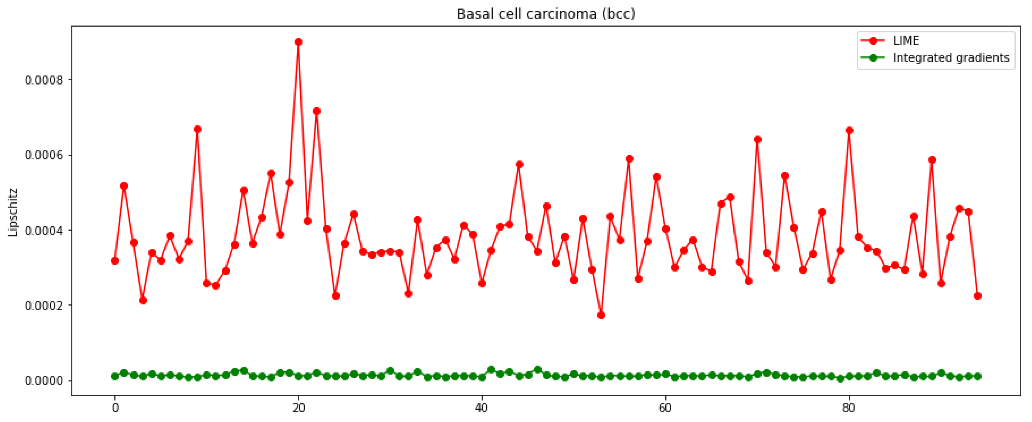
3.3. Metrics and Axioms

Table 2. Quantitative quality indicators for the different explanation techniques.

	Integrated Gradients
	akiec	bcc	bkl	df	nv	mel	vasc
Lipschitz Robustness	$0.0012$	$0.001$	$0.0014$	$0.0008$	$0.0018$	$0.0014$	$0.0012$
mean (±std)	$\pm 0.0003$	$\pm 0.0005$	$\pm 0.0004$	$\pm 0.0005$	$\pm 0.0006$	$\pm 0.0004$	$\pm 0.0005$
Stability %	100	100	100	100	100	100	100
Local Fidelity %	100	100	100	100	100	100	100
	LIME
Lipschitz Robustness	$0.0004$	$0.0004$	$0.0007$	$0.0005$	$0.0009$	$0.0004$	$0.0002$
mean (±std)	$\pm 0.0002$	$\pm 0.0001$	$\pm 0.0002$	$\pm 0.0003$	$\pm 0.0003$	$\pm 0.0001$	$\pm 0.0001$
Stability %	0	0	0	0	0	0	0
Local Fidelity %	100	100	100	100	100	100	100

reports the three quantitative quality indicators (see Section 2.2.3) for the different explanation techniques. Regarding the local fidelity, the two explanation techniques were on par; both showed full fidelity. Since the integrated gradients method uses the original model, its fidelity is by default 100%. For LIME, the local fidelity on all instances in the test set was also 100%. The local surrogate models that LIME built to explain the predictions of the test instances predicted in all 2003 cases (i.e., all observations in the test set), the same class out of the seven skin lesion classes as the original model. Note that this also means that the local surrogate model predicted the wrong class if the original model predicted the wrong class (see Figure 2 for the test set predictions).

Regarding the stability and robustness, the integrated gradient method clearly outperformed LIME. Although integrated gradients always gave the same results (feature attributions) when the explanation was repeated for the same instance and same settings (100% stability on the test set), LIME always gave a different result (0% stability on the test set).

Similarly, the integrated gradient method proved to be more robust than LIME. For all classes, the Lipschitz robustness indicator [59] was smaller (i.e., better) for the integrated gradients explanation technique than for LIME. To visualize this difference, Figure 6 shows the Lipschitz robustness indicator for the two explanation techniques, as an example, for the test instances of the basal cell carcinoma (bcc) class.

In sum, the integrated gradients explanation technique seems better with regard to the quantitative evaluation metrics. However, one should keep in mind that LIME is model-agnostic, while the integrated gradients method can only be applied if the original model is differentiable. Because of this, the LIME explainer is also more portable and can be used even if the original model would be changed.

4. Discussion and Conclusions

In this paper, we compared two currently popular XAI/IML explanation techniques applied on top of a well-performing deep CNN classification model classifying seven types of skin lesion. Both XAI/IML techniques showed a hundred percent fidelity to the original CNN model. However, integrated gradients was clearly better with regard to the other two quantitative metrics (stability and robustness). In comparison, LIME explanations were not stable (each run produced a different explanation) and less robust than the integrated gradients explanation, but the qualitative visualization seemed to use more features and were somewhat more intuitive. Moreover, in contrast to the integrated gradients, which depend on the model internals’ gradient, the LIME explainer is model-agnostic, and thus more portable and applicable also when the classification model is changed.

Limitations and Future Work

The results presented in this paper are limited by the number of models, explanation techniques, and metrics used. Moreover, they are specific to the used dataset. A plethora of different explanation techniques exists and although we used explanation techniques from two different branches (see Section 2.2.2), that is, one gradient-based model-dependent and one perturbation-based model-agnostic, there are many more XAI/IML techniques that would be interesting to compare.

In particular, it would be interesting to build easier, more traditional classification models with manual feature engineering in future work, and compare the hand-engineered features to the automatically generated ones from the CNN. More precisely, it would be interesting to use a classifier that provides modular global feature importance, such as those that any tree-based classifier or logistic regression models supply, and analyse their differences.

Another direction for future work would be to improve the CNN model and augment the used data. In this work, we focused on the explainability techniques. However, novel approaches for medical image analysis using CNNs (see, e.g., [65]), and special strategies to deal with the imbalanced data (see, e.g., [61]), such as employing a weighted cross entropy loss function, or collecting and integrating more images of the minority classes would certainly improve the classification performance and might also yield more interpretable models. In addition, future works could also use effective techniques, such as colour constancy algorithms, to improve the quality of the over a 20-year-long period collected dermoscopic images, and should use, also, other datasets to increase the generalizability of findings. Finally, we hope that future work will follow our study and compare not only accuracy but also explainability and explanation approaches for given models.

Before an automatic AI skin lesion classification system with integrated explanation techniques can be used reliably in practice, future work should also look into which explanation should be offered if several, maybe even conflicting ones, are available. As a whole, this papers offers a framework for building an explainable AI skin cancer classification system, but a set of questions, including legal ones, remain to be answered before such a system could be integrated into clinical practice.

References

1. Cassidy, B.; Kendrick, C.; Brodzicki, A.; Jaworek-Korjakowska, J.; Yap, M.H. Analysis of the ISIC image datasets: Usage, benchmarks and recommendations. Med. Image Anal. 2022, 75, 102305. [Google Scholar] [CrossRef]
2. Esteva, A.; Kuprel, B.; Novoa, R.A.; Ko, J.; Swetter, S.M.; Blau, H.M.; Thrun, S. Dermatologist-level classification of skin cancer with deep neural networks. Nature 2017, 542, 115–118. [Google Scholar] [CrossRef]
3. Holland, K. What Is a Dermatologist and How Can They Help You? Healthline. 2020. Last Medically Reviewed on 24 June 2020. Available online: https://www.healthline.com/find-care/articles/dermatologists/what-is-a-dermatologist (accessed on 22 September 2022).
4. Shen, D.; Wu, G.; Suk, H.I. Deep learning in medical image analysis. Annu. Rev. Biomed. Eng. 2017, 19, 221. [Google Scholar] [CrossRef]
5. Barata, C.; Celebi, M.E.; Marques, J.S. Explainable skin lesion diagnosis using taxonomies. Pattern Recognit. 2021, 110, 107413. [Google Scholar] [CrossRef]
6. Thurnhofer-Hemsi, K.; Domínguez, E. A convolutional neural network framework for accurate skin cancer detection. Neural Process. Lett. 2021, 53, 3073–3093. [Google Scholar] [CrossRef]
7. Brinker, T.J.; Hekler, A.; Enk, A.H.; Klode, J.; Hauschild, A.; Berking, C.; Schilling, B.; Haferkamp, S.; Schadendorf, D.; Fröhling, S.; et al. A convolutional neural network trained with dermoscopic images performed on par with 145 dermatologists in a clinical melanoma image classification task. Eur. J. Cancer 2019, 111, 148–154. [Google Scholar] [CrossRef]
8. Tschandl, P.; Rinner, C.; Apalla, Z.; Argenziano, G.; Codella, N.; Halpern, A.; Janda, M.; Lallas, A.; Longo, C.; Malvehy, J.; et al. Human–computer collaboration for skin cancer recognition. Nat. Med. 2020, 26, 1229–1234. [Google Scholar] [CrossRef]
9. Haggenmüller, S.; Maron, R.C.; Hekler, A.; Utikal, J.S.; Barata, C.; Barnhill, R.L.; Beltraminelli, H.; Berking, C.; Betz-Stablein, B.; Blum, A.; et al. Skin cancer classification via convolutional neural networks: Systematic review of studies involving human experts. Eur. J. Cancer 2021, 156, 202–216. [Google Scholar] [CrossRef]
10. Codella, N.C.; Lin, C.C.; Halpern, A.; Hind, M.; Feris, R.; Smith, J.R. Collaborative human-AI (CHAI): Evidence-based interpretable melanoma classification in dermoscopic images. In Understanding and Interpreting Machine Learning in Medical Image Computing Applications; Springer: Cham, Germany, 2018; pp. 97–105. [Google Scholar]
11. Selvaraju, R.R.; Cogswell, M.; Das, A.; Vedantam, R.; Parikh, D.; Batra, D. Grad-cam: Visual explanations from deep networks via gradient-based localization. In Proceedings of the IEEE International Conference on Computer Vision, Venice, Italy, 22–29 October 2017; pp. 618–626. [Google Scholar]
12. Maron, R.C.; Schlager, J.G.; Haggenmüller, S.; von Kalle, C.; Utikal, J.S.; Meier, F.; Gellrich, F.F.; Hobelsberger, S.; Hauschild, A.; French, L.; et al. A benchmark for neural network robustness in skin cancer classification. Eur. J. Cancer 2021, 155, 191–199. [Google Scholar] [CrossRef] [PubMed]
13. Tschandl, P.; Rosendahl, C.; Kittler, H. The HAM10000 dataset, a large collection of multi-source dermatoscopic images of common pigmented skin lesions. Sci. Data 2018, 5, 180161. [Google Scholar] [CrossRef]
14. Gaube, S.; Suresh, H.; Raue, M.; Merritt, A.; Berkowitz, S.J.; Lermer, E.; Coughlin, J.F.; Guttag, J.V.; Colak, E.; Ghassemi, M. Do as AI say: Susceptibility in deployment of clinical decision-aids. NPJ Digit. Med. 2021, 4, 31. [Google Scholar] [CrossRef]
15. Adadi, A.; Berrada, M. Peeking inside the black-box: A survey on explainable artificial intelligence (XAI). IEEE Access 2018, 6, 52138–52160. [Google Scholar] [CrossRef]
16. Arrieta, A.B.; Díaz-Rodríguez, N.; Del Ser, J.; Bennetot, A.; Tabik, S.; Barbado, A.; García, S.; Gil-López, S.; Molina, D.; Benjamins, R.; et al. Explainable Artificial Intelligence (XAI): Concepts, taxonomies, opportunities and challenges toward responsible AI. Inf. Fusion 2020, 58, 82–115. [Google Scholar] [CrossRef]
17. Guidotti, R.; Monreale, A.; Ruggieri, S.; Turini, F.; Giannotti, F.; Pedreschi, D. A survey of methods for explaining black box models. ACM Comput. Surv. (CSUR) 2018, 51, 1–42. [Google Scholar] [CrossRef]
18. Samek, W.; Montavon, G.; Lapuschkin, S.; Anders, C.J.; Müller, K.R. Explaining deep neural networks and beyond: A review of methods and applications. Proc. IEEE 2021, 109, 247–278. [Google Scholar] [CrossRef]
19. Tjoa, E.; Guan, C. A survey on explainable artificial intelligence (XAI): Toward medical XAI. IEEE Trans. Neural Netw. Learn. Syst. 2020, 32, 4793–4813. [Google Scholar] [CrossRef]
20. Sundararajan, M.; Taly, A.; Yan, Q. Axiomatic attribution for deep networks. In Proceedings of the International Conference on Machine Learning, Sydney, Australia, 6–11 August 2017; pp. 3319–3328. [Google Scholar]
21. Ribeiro, M.T.; Singh, S.; Guestrin, C. “Why Should I Trust You?”: Explaining the Predictions of Any Classifier. In Proceedings of the 22nd ACM SIGKDD International Conference on Knowledge Discovery and Data Mining, San Francisco, CA, USA, 13–17 August 2016; pp. 1135–1144. [Google Scholar]
22. Saarela, M.; Jauhiainen, S. Comparison of feature importance measures as explanations for classification models. SN Appl. Sci. 2021, 3, 272. [Google Scholar] [CrossRef]
23. Saarela, M.; Kärkkäinen, T. Can we automate expert-based journal rankings? Analysis of the Finnish publication indicator. J. Inf. 2020, 14, 101008. [Google Scholar] [CrossRef]
24. Zhang, J.; Xie, Y.; Xia, Y.; Shen, C. Attention residual learning for skin lesion classification. IEEE Trans. Med. Imaging 2019, 38, 2092–2103. [Google Scholar] [CrossRef]
25. Höhn, J.; Hekler, A.; Krieghoff-Henning, E.; Kather, J.N.; Utikal, J.S.; Meier, F.; Gellrich, F.F.; Hauschild, A.; French, L.; Schlager, J.G.; et al. Integrating patient data into skin cancer classification using convolutional neural networks: Systematic review. J. Med. Internet Res. 2021, 23, e20708. [Google Scholar] [CrossRef]
26. Gulzar, Y.; Khan, S.A. Skin Lesion Segmentation Based on Vision Transformers and Convolutional Neural Networks—A Comparative Study. Appl. Sci. 2022, 12, 5990. [Google Scholar] [CrossRef]
27. Ali, M.S.; Miah, M.S.; Haque, J.; Rahman, M.M.; Islam, M.K. An enhanced technique of skin cancer classification using deep convolutional neural network with transfer learning models. Mach. Learn. Appl. 2021, 5, 100036. [Google Scholar] [CrossRef]
28. Ali, K.; Shaikh, Z.A.; Khan, A.A.; Laghari, A.A. Multiclass skin cancer classification using EfficientNets—A first step towards preventing skin cancer. Neurosci. Inform. 2021, 2, 100034. [Google Scholar] [CrossRef]
29. Ali, R.; Hardie, R.C.; Narayanan, B.N.; De Silva, S. Deep learning ensemble methods for skin lesion analysis towards melanoma detection. In Proceedings of the 2019 IEEE National Aerospace and Electronics Conference (NAECON), Dayton, OH, USA, 15–19 July 2019; pp. 311–316. [Google Scholar]
30. Klaise, J.; Van Looveren, A.; Vacanti, G.; Coca, A. Alibi Explain: Algorithms for Explaining Machine Learning Models. J. Mach. Learn. Res. 2021, 22, 181-1. [Google Scholar]
31. LeCun, Y.; Bengio, Y.; Hinton, G. Deep learning. Nature 2015, 521, 436–444. [Google Scholar] [CrossRef]
32. Deng, L.; Yu, D. Deep learning: Methods and applications. Found. Trends Signal Process. 2014, 7, 197–387. [Google Scholar] [CrossRef]
33. Qin, Z.; Yu, F.; Liu, C.; Chen, X. How convolutional neural network see the world-A survey of convolutional neural network visualization methods. Math. Found. Comput. 2018, 1, 149–180. [Google Scholar] [CrossRef]
34. Khan, S.A.; Gulzar, Y.; Turaev, S.; Peng, Y.S. A Modified HSIFT Descriptor for Medical Image Classification of Anatomy Objects. Symmetry 2021, 13, 1987. [Google Scholar] [CrossRef]
35. Valueva, M.V.; Nagornov, N.; Lyakhov, P.A.; Valuev, G.V.; Chervyakov, N.I. Application of the residue number system to reduce hardware costs of the convolutional neural network implementation. Math. Comput. Simul. 2020, 177, 232–243. [Google Scholar] [CrossRef]
36. Albawi, S.; Mohammed, T.A.; Al-Zawi, S. Understanding of a convolutional neural network. In Proceedings of the IEEE 2017 International Conference on Engineering and Technology (ICET), Antalya, Turkey, 21–23 August 2017; pp. 1–6. [Google Scholar]
37. Molnar, C. Interpretable Machine Learning: A Guide for Making Black Box Models Explainable, 2nd ed.; Lulu Press: Morrisville, NC, USA, 2022. [Google Scholar]
38. Carvalho, D.V.; Pereira, E.M.; Cardoso, J.S. Machine learning interpretability: A survey on methods and metrics. Electronics 2019, 8, 832. [Google Scholar] [CrossRef]
39. Doshi-Velez, F.; Kim, B. Towards a rigorous science of interpretable machine learning. arXiv 2017, arXiv:1702.08608. [Google Scholar]
40. Miller, T. Explanation in artificial intelligence: Insights from the social sciences. Artif. Intell. 2019, 267, 1–38. [Google Scholar] [CrossRef]
41. Koh, P.W.; Liang, P. Understanding black-box predictions via influence functions. In Proceedings of the 34th International Conference on Machine Learning, Sydney, Australia, 6–11 August 2017; Volume 70. [Google Scholar]
42. Yeh, C.K.; Kim, J.; Yen, I.E.H.; Ravikumar, P.K. Representer point selection for explaining deep neural networks. Adv. Neural Inf. Process. Syst. 2018, 31, 1–11. [Google Scholar]
43. Li, O.; Liu, H.; Chen, C.; Rudin, C. Deep Learning for Case-Based Reasoning through Prototypes: A Neural Network that Explains Its Predictions. In Proceedings of the Thirty-Second AAAI Conference on Artificial Intelligence, New Orleans, LA, USA, 2–7 February 2018. [Google Scholar]
44. Wachter, S.; Mittelstadt, B.; Russell, C. Counterfactual Explanations without Opening the Black Box: Automated Decisions and the GDPR. Harv. J. Law Technol. 2017, 31, 841. [Google Scholar] [CrossRef]
45. Erhan, D.; Bengio, Y.; Courville, A.; Vincent, P. Visualizing higher-layer features of a deep network. Univ. Montr. 2009, 1341, 1. [Google Scholar]
46. Towell, G.G.; Shavlik, J.W. Extracting refined rules from knowledge-based neural networks. Mach. Learn. 1993, 13, 71–101. [Google Scholar] [CrossRef]
47. Castro, J.L.; Mantas, C.J.; Benitez, J.M. Interpretation of artificial neural networks by means of fuzzy rules. IEEE Trans. Neural Netw. 2002, 13, 101–116. [Google Scholar] [CrossRef] [PubMed]
48. Mitra, S.; Hayashi, Y. Neuro-fuzzy rule generation: Survey in soft computing framework. IEEE Trans. Neural Netw. 2000, 11, 748–768. [Google Scholar] [CrossRef] [PubMed]
49. Fisher, A.; Rudin, C.; Dominici, F. All Models are Wrong, but Many are Useful: Learning a Variable’s Importance by Studying an Entire Class of Prediction Models Simultaneously. J. Mach. Learn. Res. 2019, 20, 1–81. [Google Scholar]
50. Fong, R.C.; Vedaldi, A. Interpretable explanations of black boxes by meaningful perturbation. In Proceedings of the IEEE International Conference on Computer Vision, Venice, Italy, 22–29 October 2017. [Google Scholar]
51. Zintgraf, L.M.; Cohen, T.S.; Adel, T.; Welling, M. Visualizing deep neural network decisions: Prediction difference analysis. In Proceedings of the International Conference on Learning Representations (ICLR), Toulon, France, 24–26 April 2017; pp. 1–12. [Google Scholar]
52. Zeiler, M.D.; Fergus, R. Visualizing and understanding convolutional networks. In Proceedings of the European Conference on Computer Vision, Zurich, Switzerland, 6–12 September 2014. [Google Scholar]
53. Wojtas, M.; Chen, K. Feature Importance Ranking for Deep Learning. In Proceedings of the Advances in Neural Information Processing Systems (NIPS 2020), Virtual, 6–12 December 2020; Volume 33, pp. 5105–5114. [Google Scholar]
54. Burkart, N.; Huber, M.F. A Survey on the Explainability of Supervised Machine Learning. J. Artif. Intell. Res. 2021, 70, 245–317. [Google Scholar] [CrossRef]
55. Dimopoulos, Y.; Bourret, P.; Lek, S. Use of some sensitivity criteria for choosing networks with good generalization ability. Neural Process. Lett. 1995, 2, 1–4. [Google Scholar] [CrossRef]
56. Simonyan, K.; Vedaldi, A.; Zisserman, A. Deep inside convolutional networks: Visualising image classification models and saliency maps. arXiv 2013, arXiv:1312.6034. [Google Scholar]
57. Shrikumar, A.; Greenside, P.; Kundaje, A. Learning important features through propagating activation differences. In Proceedings of the International Conference on Machine Learning, Sydney, Australia, 6–11 August 2017; pp. 3145–3153. [Google Scholar]
58. Vilone, G.; Longo, L. Notions of explainability and evaluation approaches for explainable artificial intelligence. Inf. Fusion 2021, 76, 89–106. [Google Scholar] [CrossRef]
59. Alvarez-Melis, D.; Jaakkola, T.S. On the robustness of interpretability methods. In Proceedings of the 35th International Conference on Machine Learning (ICML 2018), Stockholm, Sweden, 10–15 July 2018. [Google Scholar]
60. Honegger, M. Shedding light on black box machine learning algorithms: Development of an axiomatic framework to assess the quality of methods that explain individual predictions. arXiv 2018, arXiv:1808.05054. [Google Scholar]
61. Saarela, M.; Ryynänen, O.P.; Äyrämö, S. Predicting hospital associated disability from imbalanced data using supervised learning. Artif. Intell. Med. 2019, 95, 88–95. [Google Scholar] [CrossRef] [PubMed]
62. Krizhevsky, A.; Sutskever, I.; Hinton, G.E. Imagenet classification with deep convolutional neural networks. Adv. Neural Inf. Process. Syst. 2012, 25, 84–90. [Google Scholar] [CrossRef]
63. Dindorf, C.; Konradi, J.; Wolf, C.; Taetz, B.; Bleser, G.; Huthwelker, J.; Werthmann, F.; Bartaguiz, E.; Kniepert, J.; Drees, P.; et al. Classification and automated interpretation of spinal posture data using a pathology-independent classifier and explainable artificial intelligence (XAI). Sensors 2021, 21, 6323. [Google Scholar] [CrossRef] [PubMed]
64. IMDRF SaMD Working Group. Software as a Medical Device(SaMD): Clinical Evaluation—Guidance for Industry and Food and Drug Administration Staff; International Medical Device Regulators Forum, Food and Drug Administration (FDA): Rockville, MD, USA, 2017.
65. Ali, R.; Hardie, R.C.; Narayanan, B.N.; Kebede, T.M. IMNets: Deep Learning Using an Incremental Modular Network Synthesis Approach for Medical Imaging Applications. Appl. Sci. 2022, 12, 5500. [Google Scholar] [CrossRef]
Figure 1. Example images from the seven different classes of skin lesion. For each class (from top to bottom row: askiec, bcc, bkl, df, mel, nv, and vasc), five randomly sampled instances are shown.
Applsci 12 09545 g001
Figure 2. Classification result (confusion matrix) of the test set on the trained CNN model.
Applsci 12 09545 g002
Figure 3. Percentage of correct classifications per class.
Applsci 12 09545 g003
Figure 4. Attribution maps/visual explanation of the explanation techniques for the true positive with the highest probability in the test set for each class. From left to right: original preprocessed image of the class, integrated gradient explanation, integrated gradient explanation overlayed on the true positive image, LIME explanation, LIME explanation overlayed on the true positive image.
Applsci 12 09545 g004
Figure 5. Attribution maps/visual explanation of the explanation techniques for those images in the test set that the classifier misclassified with the highest probability. From left to right: original preprocessed image of the class that the classifier misclassified with the highest probability, integrated gradient explanation, integrated gradient explanation overlayed on the misclassified image, LIME explanation, LIME explanation overlayed on the misclassified image.
Applsci 12 09545 g005
Figure 6. Lipschitz robustness estimate for LIME and integrated gradient explanations for test instances of the basal cell carcinoma (bcc) class. The explanations of the integrated gradient technique are clearly robuster than the LIME explanations.
Applsci 12 09545 g006