Article

Classification of Road Surfaces Based on CNN Architecture and Tire Acoustical Signals

1
Acoustic and Vibration Signal Processing Laboratory, Department of Mechanical Engineering, INHA University, Incheon 22212, Korea
2
HYUNDAI Motor Company, Seoul 137938, Korea
3
NEXEN Tire Corporation, Yangsan 626230, Korea
*
Author to whom correspondence should be addressed.
Appl. Sci. 2022, 12(19), 9521; https://doi.org/10.3390/app12199521
Submission received: 18 August 2022 / Revised: 16 September 2022 / Accepted: 20 September 2022 / Published: 22 September 2022
(This article belongs to the Special Issue Recent Automotive Noise Vibration Harshness (NVH) and Sound Quality)

Abstract

:
This paper presents a novel work for classification of road surfaces using deep learning method-based convolutional neural network (CNN) architecture. With the development of advanced driver assistance system (ADAS) and autonomous driving technologies, the need for research on vehicle state recognition has increased. However, research on road surface classification has not yet been conducted. If road surface classification and recognition are possible, the control system can make a more robust decision by validating the information from other sensors. Therefore, road surface classification is essential. To achieve this, tire-pavement interaction noise (TPIN) is adopted as a data source for road surface classification. Accelerometers and vision sensors have been used in conventional approaches. The disadvantage of acceleration signals is that they can only represent the surface profile properties and are masked by the resonance characteristics of the car structure. An image signal can be easily contaminated by factors such as illumination, obstacles, and blurring while driving. However, the TPIN signal reflects the surface profile properties of the road and its texture properties. The TPIN signal is also robust compared to those in which the image signal is affected. The measured TPIN signal is converted into a 2-dimensional image through time–frequency analysis. Converted images were used together with a CNN architecture to examine the feasibility of the road surface classification system.

1. Introduction

The tire is a key part where direct contact occurs between the road surface and the automobile. The tires and road surfaces are directly related to the braking performance of the vehicle. For the safety of driver and passengers, braking performance is important. In the winter season, the friction between road surface and tire depends on the condition of road surfaces such as asphalt roads with snow or without snow. Therefore, studies regarding road tire friction estimation have been conducted for decades [1,2,3]. Particularly, it is necessary for autonomous cars to estimate the friction in real time for the car. However, it is difficult to estimate the friction in real time directly. In this work, as an indirection method instead of a direct measurement of friction, a new CNN) architecture to classify the road surface in real time is proposed based on deep learning of the acoustic signal generated by the contact between tire and road surface during driving. In previous studies on road surface classification, various combinations of sensors and algorithms were used to identify road surfaces. The microphone and support vector machine combination has been used to classify dry and wet road surface conditions [4]. Other research measured acoustic noise signals from the tire cavity space to identify road surface types [5]. Road surface image data have also been used for road surface classification based on hyperspectral image processing [6] and convolutional neural network (CNN) architecture [7]. Despite many approaches and studies, there have been no studies on the classification of snow-covered roads that require precise brake control. Therefore, research identifying road surfaces by considering tire patterns is required to increase the robustness of the control system. In this study, a new road surface classification method that includes snow road is presented based on a tire–pavement interaction noise (TPIN) signal and a deep learning train using a CNN architecture. Two tires made by two different companies and two road surfaces were used for this method. Thus, there were four classes. The aim of this study is to determine if the road has snow on the road to use the results for safety analysis autonomous driving technologies in the future. The effect of tire type is considered for this classification. The TPIN signal is obtained using a rugged microphone installed on the wheel cover, and it is transformed into 2-dimensional (2D) image data using continuous wavelet transform (CWT). The image signal is used as the input to the CNN architecture. A new CNN architecture was constructed for the classification of two road surface types and two tires. The remainder of this paper is organized as follows. Section 2 contains fundamental theories regarding CWT, convolutional neural networks, and TPIN. Section 3 presents the experimental setup, test environment, and result analysis. Section 4 focuses on the preprocessing technique and a comparison of the resulting CWT images. Section 5 addresses the design of the neural network, training setup, and network performance. Finally, Section 6 discusses the overall research process.

2. Background Theory

2.1. Continuous Wavelet Transform (CWT)

CWT is a method used for time–frequency domain analysis. It can overcome the fixed-resolution problem of the short-time Fourier transform (STFT). The STFT has the same resolution throughout the frequency ranges because of the fixed window size. The CWT can have a different resolution by adjusting its basis functions. The difference in the window between the STFT and CWT is illustrated in Figure 1. The CWT is defined using Equation (1) [8].
W b ( a ) = < ψ a , b * ( t ) , x ( t ) | a | 1 2 x ( t ) ψ a , b * d t   where   ψ a , b ( t ) = ψ ( t b a )
In Equation (1), x ( t ) is an arbitrary input signal, and ψ ( t ) is the mother wavelet or basis function. Along with the type of basis function, ψ ( t ) can take various forms. ψ a , b * is a complex conjugate of ψ a , b ( t ) , where ψ a , b ( t ) is the dilated and translated version of the mother wavelet ψ ( t ) . The parameter a is a dilation factor. The parameter b is a translation factor that controls the amount of translation along the time axis. In addition to the dilation and translation factors, the type of mother wavelet itself is an important parameter of the CWT. This study uses a Morlet wavelet, which is defined in Equation (2), for the mother wavelet. The coordinates of the center point of the mother wavelet in the time–frequency domain are ( 0 ,   η / 2 π ) . For example, if η = 6 , the t-axis coordinate of the center point is 0. The y-axis coordinate (also called the central frequency, μ f ) was 6 / ( 2 π ) . Further discussion about the theory and another application case of the continuous wavelet transform can be found in [9,10].
ψ ( t ) = π 1 4 exp ( t 2 2 + j η t )

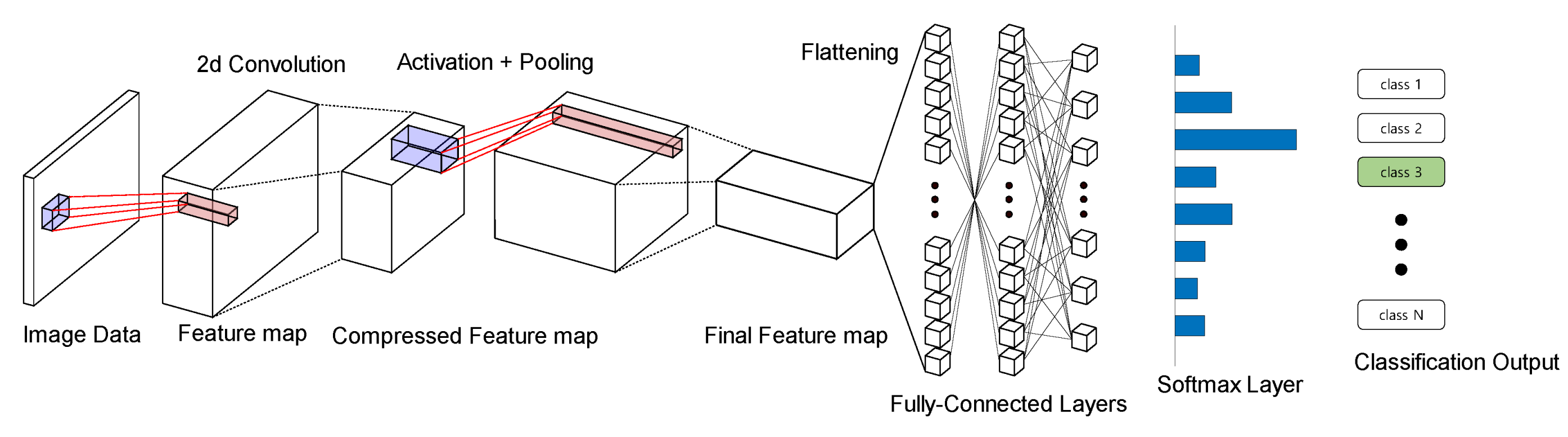
2.2. Convolutional Neural Network (CNN)

CNN is a type of artificial neural network that optimizes weights based on an input image feature map. The feature map is extracted through a convolution operation between the input data and a predefined convolution kernel. CNN is widely known for its excellent performance in various image-recognition tasks. Recently, CNN techniques have been applied in various fields of mechanical engineering. Defect classification of power driving systems, prediction of tire-transmitted noise, and vehicle structure defect classification are successful applications in mechanical engineering [11,12,13]. The modern concept of CNN was first suggested by LeCun et al. [14]. In that paper, Yann LeCun introduced LeNet-5 to recognize letter patterns. LeNet-5 uses a convolution operation on a 32 × 32-pixel input image to achieve this goal. The feature map is then compressed using a pooling operation. After repeating the above process twice, the final feature map was unfolded to flatten and connected to a fully connected layer. The number of nodes in the last fully connected layer was equal to the number of classes. The values at each node were normalized between 0 and 1 using the softmax layer. Using this normalized score, LeNet-5 can determine the class of an input letter. These suggested procedures, from convolution, pooling, and fully connected layers to softmax layers, have become the basic architecture of CNN. Figure 2 illustrates the basic structure of a CNN similar to that of LeNet-5. For visual simplicity, only a few connections between the nodes were expressed in the fully connected layer. The following text provides a more detailed explanation of each layer’s operation.
The convolution layer is the most important feature of the CNN architecture. Typically, its output is referred to as a feature map. A feature map is a value set resulting from a convolution operation between the input data and filter. The component of i-th row and j-th column in the feature map is calculated using Equation (3) [14].
y i , j , k = b k + u = 0 f h 1 v = 0 f w 1 k = 0 f c 1 x i , j , k ω u , v , k , k  
f h and f w are the filter height and width, respectively. f c denotes the total number of channels in the input data. b k is the bias for k-th filter, x is the pixel value of the input. ω is the learnable weight of the filter. As the training proceeds, the weights in the filter are updated to effectively extract the features of the input data. The output of the convolution layer is fed to the activation layer. The activation layer determines the activation level of the fed output using a predefined activation function. To represent the complex boundaries between classes in a high-dimensional feature space, activation functions are usually defined as nonlinear functions. The most widely used activation function in recent times is the rectified linear unit (ReLu). The definition of ReLu is shown using Equation (4).
ϕ = max ( 0 , x )
In general, the activation layer is followed by a pooling layer. The pooling layer reduces the size of the feature map generated by the convolution layer. This subsampling process helps reduce the computational cost. It is also known to prevent neural networks from overfitting. The most commonly used pooling operations are max pooling and average pooling. Their mechanism is illustrated in Figure 3.
After convolution, activation, and pooling operation, the final feature map was delivered to the fully connected layer. As the name implies, every node in the previous layer is connected to every node in the next layer. First, the 3-dimensional feature map is flattened to a 1-dimensional (1D) feature vector. Except for the first conversion process, the other operations were the same as those of the multilayer perceptron. The last fully connected layer had as many nodes as the number of classes for classification. Deep neural networks used for classification tasks generally have a softmax output layer. This layer used the softmax function defined in Equation (5). o i denotes i-th node’s output value in the final fully connected layer. The output P i is the normalized probability value for i-th class. As shown in the equation, each output value passes through an exponential function. Then, each scaled value is divided by the sum of all outputs. A neural network selects the output class that has the greatest possibility, as shown in Equation (6).
P i = exp ( o i ) n = 1 k exp ( o n )
y ^ = max ( P 1 , P 2 , , P k 1 , P k )  
The training process is performed using these layers. Softmax normalizes such that the output can be viewed as the probability that the input is within the class. Once the score vector is calculated, the loss function uses the vector and ground-truth labels to calculate the loss of the input image. Updates for every learnable parameter in a neural network are determined using backpropagation and gradient descent methods. These are the typical training processes for CNN [12]. The training algorithm was developed during the development of the CNN architecture. Currently, almost all training algorithms can be categorized into two groups. The first is to adjust the gradient direction. The second is to control the step size. The gradient-direction type is good at avoiding local minima. The step-size type enables the network to learn stable. Recently, an algorithm called Adam got a lot of interest for its good performance [15]. It is a hybrid-type algorithm that combines the advantages of gradient direction and step-size type. For efficient training, Adam is used in this study instead of a conventional stochastic gradient descent algorithm. Further information on CNN can be found in various books and papers [16,17,18]. The used software for this research is Matlab (MathWorks Co., Natick, MA, USA).

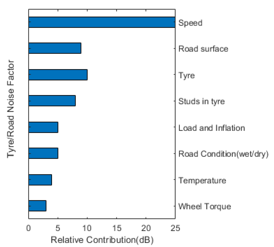
2.3. Tire-Pavement Interaction Noise

Tire-pavement interaction noise refers to the noise generated by the interaction between wheels and road surfaces while driving. There are several types of sources; for example, road induced, tire induced, road surface induced, and environment induced. Figure 4 shows the relative contributions of various influencing factors to the overall noise level of the TPIN [19]. Because there are too many details for each factor, only three dominant factors, speed, road, and tire, are considered within the required scope.
Speed plays a more important role than other factors. This means that the noise level of the TPIN is strongly affected by speed [19,20]. There are two main reasons for this finding. First, the first is the tread impact noise generated by physical contact between the tire and the road surface. The impulse level between the tire and road is proportional to the rotation speed of the tire, which is directly related to the car speed. The second is air pumping noise. The main generation mechanism of air pumping noise is the compression expansion action of air. The inflow and outflow of air into the tire groove and tread increase as the speed increases [21]. Such volume fluctuations directly induce pressure fluctuations, that is sound waves. These noises usually have a frequency range of 1000–2500 Hz. The experimental relationship between speed and TPIN is shown in Equation (7). Here, L is the acoustic pressure level, and v is the vehicle speed. A and B are coefficients that depend on environmental factors.
L = A + B   l o g ( v )
There are many other secondary effects in addition to those mentioned above. The horn effect, Helmholtz resonance, sidewall resonance, torus cavity resonance, and tire-rim assembly resonance are good examples [19,20,22]. In the road part, the roughness of the pavement texture, that is, the road texture, is worth covering. The roughness of the pavement texture indicates the extent of deviation of the surface profile from the reference plane. Pavement textures can be divided into several categories based on the texture wavelength. The microtexture had a wavelength smaller than 0.5 mm. The macro-texture’s wavelength is between 0.5 and 50 mm. The mega-texture has a wavelength range of 50–500 mm. Mega-textures are known to be the main source of noise generation.

3. Experiment

3.1. Experimental Setup and Devices

For the microphone, a GRAS 40PH 1/4 inch free-field model was used. Two microphones were used to compare the results from the front and rear wheels. Each microphone was attached to the front of the wheel housing. This position was selected to record the only sound by the tire–pavement interaction and to exclude the environment noise. The LMS SCADAS Mobile device (Siemeans, Co., Munich, Germany) was selected for the 2-channel measurement. The sampling frequency was fixed at 51,200 Hz because frequency range of tire noise is located between 500 Hz and 20 kHz. Figure 5 shows an actual picture of the experimental vehicle, microphone position, and a schematic description.

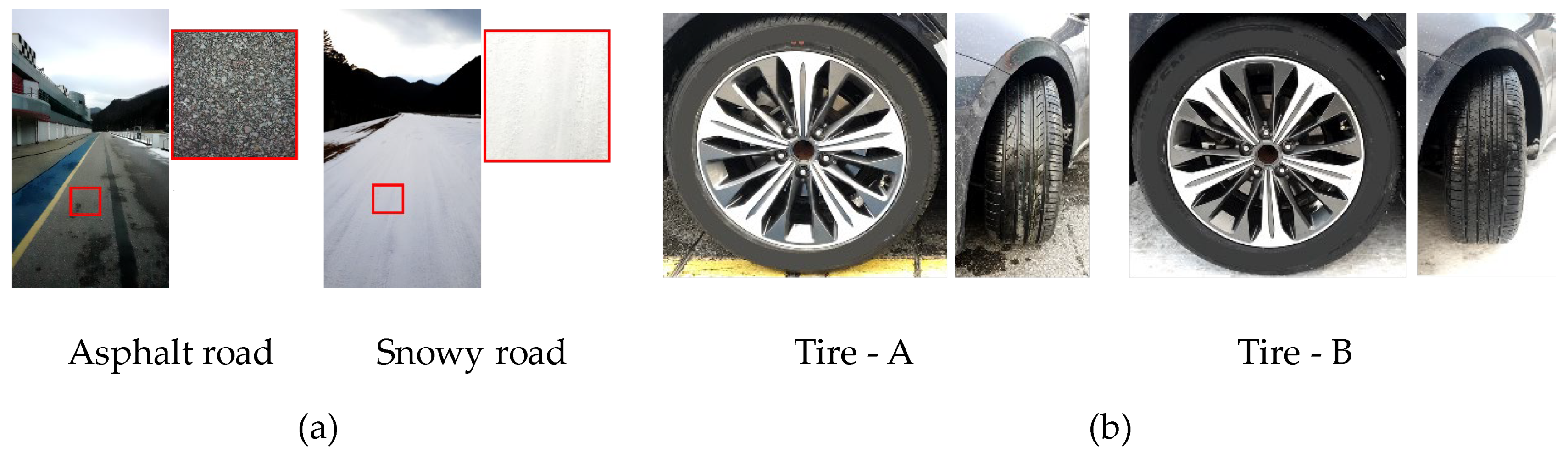
3.2. Test Roads and Tire Types

Two types of roads and two types of tires were selected for the measurement of tire–pavement interaction noise. The test car is a used passenger car with 4cylinder engine. For the winter test of tire, a wide test track is developed in the mount. During test, snow condition on the road is not changed. Types of test roads were asphalt and snowy road, both of which were straight. The only difference is that there is snow or no snow on the road. Surface roughness of test road is different according to road type. Each test road was longer than 60 m. The speed of test car is maintained at approximately 40 km/h for the safety in snowy road condition. However, there was a speed fluctuation between 35 and 45 km/h because test driver tried to keep 40 km/h manually when test was done. The snow is always fresh and no compressed. The test tires were commercial products from different companies referred to as A-company and B-company. They are all new winter model tires and have different tread shape. In this study, the tire from A-company and B-company is denoted as tire-A and tire-B, respectively. Tire-A and tire-B were tested seven times on an asphalt road. For the snowy road case, tire-A was tested 22 times, and tire-B was tested 20 times. Figure 6 illustrates the test roads and tires outlined above.

3.3. Data Acquisition and Analysis

Figure 7 shows the measured signal in the time domain for each test case. The results from the front wheel are listed in the first two rows, and those from the rear wheel are listed in the third and fourth rows. The combination of test tires and roads is notated as the title of the subplots. Figure 8 shows the corresponding frequency spectrum graphs of Figure 7. The left side of Figure 8 illustrates the results from the front wheel for all tire-road cases simultaneously, and the right side shows the results for the rear wheel similarly. As shown in Figure 8, the overall sound pressure level of the snowy road is larger than that of the asphalt road in the frequency range from 20 to 600 Hz because the sound generated while the tire compresses snow on the road contributes to the overall noise level. However, in the frequency range from 600 to 2500 Hz, the opposite situation occurs. It is estimated that various noises induced by tread impact, texture impact, and air pumping effect are significantly suppressed because tire treads and grooves are filled with snow. Finally, in the frequency range over 2500 Hz, the graphs tended to be separated along the tire type rather than the road type.

4. Data Processing

The measured noise signal must be converted into a proper image form because a CNN was utilized as a classifier in this study. A 1D noise signal is transformed into 2D time–frequency data using a signal processing technique. The 2D data are then mapped to a predefined color map to generate an image. Here, CWT was selected for the 1D to 2D transformation. CWT has a good resolution in both the time and frequency domains, which is essential for revealing the complex properties of TPIN. The better the generated image reflects the characteristics of noise, the better the CNN is likely to extract these characteristics. This is directly related to the good classification performance of the CNN. Images from the CWT were analyzed to determine a set of CWT parameters, which are time, frequency and magnitude of CWT and are independent of the neural network. For this pre-analysis, the length of the data for each case was limited to 6 s for fairness.
Figure 9 shows scaled colormap images for magnitude of CWT for 3 s data of each test sample. The color bar in right side of image shows scale for sound pressure in each image in “pa” unit. The color bar is presented by 128 integers from 0 to 127. Sound pressure is rescaled by 128 integers. For production of input data of CNN, time signal of each sample is truncated into 0.05 s with 80% overlap. CWT for the truncated signal of 0.005 s is performed and a thousand numbers of scaled images in “pa” unit per each test sample are generated as listed in Table 1. Since road surface is random during driving, 11,040 images are randomly arranged for the input of CNN. These images are normalized within range [0, 1] and transformed to RGB images. This RGB image is composed of 3 layers and is resized to 224 × 224 × 3 pixels. By comparing snow and asphalt roads in the frequency range of 20–600 Hz, the overall noise level difference appears, as indicated in the frequency spectrum analysis. The TPIN property of the asphalt road was well reflected in the 800–1000 Hz frequency range. The CWT data were scaled and mapped into an RGB color map. The final procedure is image resizing. The dimensions of the final image were 224 × 224 × 3 pixels in the order of height, width, and channel. An example of the final image is shown in Figure 10. In the case of asphalt, the effect of road texture is emphasized. The component of the low-frequency region was well visualized in the snowy road case.

5. Training of Neural Network

5.1. Dataset Preparation

Table 1 lists the total number of images generated for each test case. The number of images is equal regardless of the tire position if the tire type and road type are unchanged. This is because the front-wheel data and rear-wheel data are measured simultaneously and controlled by the same digital signal processor mentioned in Section 3.1. Consequently, the length of the acquired data was the same for every measurement. The procedures used to create the final dataset were as follows. First, randomly extract approximately 4000 images for each class. Second, it was divided into three subsets: one for training, another for validation, and the other for testing. The training set uses approximately 60% of the total image, validation set uses approximately 20%, and test set takes the remaining. Third, the first two steps are repeated for all test cases. Finally, the created datasets of the same type are merged. Two final datasets were created individually from the front-wheel and rear-wheel data.

5.2. Architecture of Network and Parameter Setup

The architecture of the CNN is simple because deep layers are not required from the results of the pre-analysis, and the computational cost needs to be reduced as much as possible for real-time applications. A schematic of the neural network architecture used for road surface classification is illustrated in Figure 11. The input size of 2D image is 224 × 224 × 3 and output classes is 4. Except for the input and output layers, the network was mainly composed of two structurally identical modules that played the same role. It is composed of a 2D convolutional layer with 16 filter sizes and 32 filter size, respectively, and an average pooling layer with 16 filter sizes and 32 filter size, respectively. ReLU activation function is used to extract the feature map in each layer. It is generally accepted that the batch normalization layer can prevent overfitting and reduce the initial weight effect [23]. Other non-learnable parameters of layers, for example, convolution filter size and pooling size, were optimized by the trial and error method for our application.
The values of several hyperparameters used for training are listed in Table 2. They are adjusted using the grid search method, which is widely used to tune hyperparameters.

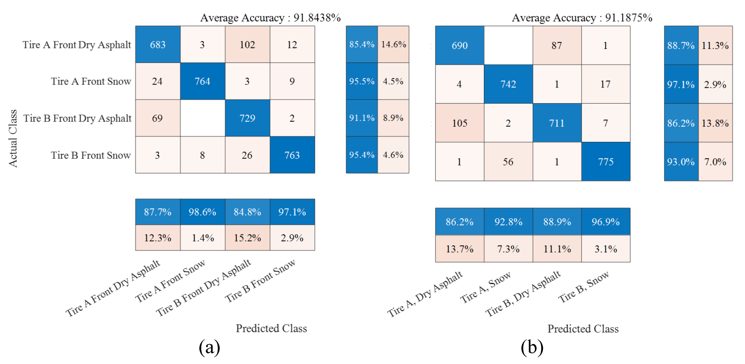
5.3. Train and Results

Figure 12 shows the convergence curve of loss during train process of 4 class classification of road surface using front-wheel data. Accuracy curve is also converged to 100% during training process. Train process is well completed. The test results are visualized in the form of a confusion chart, as shown in Figure 13. The diagonal elements in the confusion chart indicate the number of correctly classified images. This implies that the predicted class label coincides with the ground-truth label of the image. Horizontally arranged percentage values with blue colored background are called accuracy, and vertically arranged ones are called precision.
As next work, to know it is possible for the CNN architecture to classify snowy road and asphalt roads even if patterns of tire are different, test data of two tires are mixed, and two classes classification is performed. Figure 14 shows confusion chart for two classes classification for snowy road and asphalt road. These results show it is possible to classify the road surface when tires are different.

6. Discussion

In this study, a road surface and tire type classification framework is suggested. First, the TPIN was measured through a microphone attached to the front side of the wheel housing. The acquired signal is then transformed and converted into 2-dimensional image data. During these processes, the temporal and nonperiodic properties of the noise signal are revealed. This is shown by comparing the CWT images of each case in Section 4. Images from the CWT were analyzed to determine a set of CWT parameters, which are time, frequency and magnitude of CWT and are independent of the neural network. A number of images are made throughput CWT of measured data. Since road surface is random during driving, 11,040 images are randomly arranged for the input of CNN. Next, a convolutional neural network was used to classify them. The depth of the neural network was determined by considering both the parameter capacity and the computational cost. It was confirmed that the final network could classify four classes with an average accuracy of more than 90%. The overall sound pressure level of the snowy road is larger than that of the asphalt road in the frequency range from 20 to 600 Hz. However, in the frequency range from 600 to 2500 Hz, the opposite situation occurs. Finally, in the frequency range over 2500 Hz, the graphs tended to be separated along the tire type rather than the road type. Tradition method is to use the spectrum difference based on the 1D spectrum data as shown in Figure 8. Traditional method cannot identify the difference of sound pressure spectrum in instant time. Therefore, in this study, CNN was used to find this difference based on 2D images data obtained by CWT and results the clear classification of road surface. CNN uses several different 2D images and classifies the images through the process of convolution, polling and softmax function.

7. Conclusions

In this work, a road surface classification method based on CNN architecture is proposed, which enables friction to estimate indirectly in real time instead of a direct measurement of friction. It proposes a new method of estimating road surfaces according to the sound pressure level and frequency band of the acoustic signal measured near to the tire. CWT is employed for frequency band analysis and sound pressure identification of the acoustic signal. CWT results for the acoustic signal are 2D images presented in the time axis and the frequency axis. CWT images for the measured acoustic signal in real time are used to input data of CNN architecture for real-time classification of road surfaces. For this study, two groups of tires manufactured by two different companies and two road surfaces such as asphalt roads with snow and without snow were considered. CNN architecture shows a superior performance for classification of four classes. These results explain that CNN architecture enables friction to estimate indirectly in real time according to the classification of road surfaces. To remove the effect of tire types, classification of two classes is performed by combining data classified by tire types. Classification of two classes for road surfaces such as asphalt roads with snow and without snow is also successfully performed. The proposed method can be used for the indirect display of estimation of friction according to road surfaces in real time.

Author Contributions

Conceptualization, S.-K.L. and Y.Y.; methodology, S.-K.L.; software, C.-H.L. and J.Y.; validation, S.-U.H. and Y.Y.; formal analysis, C.-H.L. and J.Y.; investigation, H.-M.J.; resources, S.-U.H.; data curation, C.-H.L. and J.Y.; writing—original draft preparation, C.-H.L. and J.Y.; writing—review and editing, S.-K.L.; visualization, J.Y.; supervision, J.L.; project administration, K.Y.; funding acquisition, K.Y. and Y.Y. All authors have read and agreed to the published version of the manuscript.

Funding

This work was supported by the National Research Foundation of Korea (NRF) grant funded by the Korea government (MSIT) (No. 2022R1F1A1062889). This study was partly supported by the HYUNDAI Motor Company and the NEXEN Tire Corporation.

Conflicts of Interest

The authors declare no conflict of interest.

References

  1. Müller, S.; Uchanski, M.; Hedrick, K. Estimation of the maximum tire-road friction coefficient. J. Dyn. Syst. Meas. Control 2003, 125, 607–617. [Google Scholar] [CrossRef]
  2. Ribeiro, A.M.; Moutinho, A.; Fioravanti, A.R.; de Paiva, E.C. Estimation of tire–road friction for road vehicles: A time delay neural network approach. J. Braz. Soc. Mech. Sci. Eng. 2020, 42, 4. [Google Scholar] [CrossRef]
  3. Rajamani, R.; Piyabongkarn, N.; Lew, J.; Yi, K.; Phanomchoeng, G. Tire-road friction-coefficient estimation. IEEE Control Syst. Mag. 2010, 30, 54–69. [Google Scholar]
  4. Alonso, J.; López, J.; Pavón, I.; Recuero, M.; Asensio, C.; Arcas, G.; Bravo, A. On-board wet road surface identification using tyre/road noise and support vector machines. Appl. Acoust. 2014, 76, 407–415. [Google Scholar] [CrossRef]
  5. Masino, J.; Pinay, J.; Reischl, M.; Gauterin, F. Road surface prediction from acoustical measurements in the tire cavity using support vector machine. Appl. Acoust. 2017, 125, 41–48. [Google Scholar] [CrossRef]
  6. Nolte, M.; Kister, N.; Maurer, M. Assessment of deep convolutional neural networks for road surface classification. In Proceedings of the 2018 21st International Conference on Intelligent Transportation Systems (ITSC), Maui, HI, USA, 4–7 November 2018; pp. 381–386. [Google Scholar]
  7. Mohammadi, M. Road classification and condition determination using hyperspectral imagery. Int. Arch. Photogramm. Remote Sens. Spat. Inf. Sci. 2012, 39, B7. [Google Scholar] [CrossRef]
  8. Lee, S.K. Improvement of impact noise in a passenger car utilizing sound metric based on wavelet transform. J. Sound Vib. 2010, 329, 3606–3619. [Google Scholar] [CrossRef]
  9. Aguiar-Conraria, L.; Azevedo, N.; Soares, M.J. Using wavelets to decompose the time–frequency effects of monetary policy. Phys. A Stat. Mech. Appl. 2008, 387, 2863–2878. [Google Scholar] [CrossRef]
  10. Addison, P.S. The Illustrated Wavelet Transform Handbook: Introductory Theory and Applications in Science, Engineering, Medicine and Finance; CRC Press: Boca Raton, FL, USA, 2017. [Google Scholar]
  11. Lee, S.-Y.; Lee, S.-K. Deep convolutional neural network with new training method and transfer learning for structural fault classification of vehicle instrument panel structure. J. Mech. Sci. Technol. 2020, 34, 4489–4498. [Google Scholar] [CrossRef]
  12. Kim, S.; An, K.; Back, J.; Lee, S.-K.; Lee, C.; Kim, P. Health Monitoring of Power Driving System Using Sound Signal based on Deep Learning. Korean Soc. Noise Vib. Eng. 2021, 31, 47–56. [Google Scholar] [CrossRef]
  13. Lee, S.-K.; Lee, H.; Back, J.; An, K.; Yoon, Y.; Yum, K.; Hwang, S.-U. Prediction of tire pattern noise in early design stage based on convolutional neural network. Appl. Acoust. 2021, 172, 107617. [Google Scholar] [CrossRef]
  14. LeCun, Y.; Bottou, L.; Bengio, Y.; Haffner, P. Gradient-based learning applied to document recognition. Proc. IEEE 1998, 86, 2278–2324. [Google Scholar] [CrossRef]
  15. Kingma, D.P.; Ba, J. Adam: A method for stochastic optimization. arXiv 2014, arXiv:1412.6980. [Google Scholar]
  16. Agarap, A.F. Deep learning using rectified linear units (relu). arXiv 2018, arXiv:1803.08375. [Google Scholar]
  17. Géron, A. Hands-On Machine Learning with Scikit-Learn, Keras, and TensorFlow: Concepts, Tools, and Techniques to Build Intelligent Systems; O’Reilly Media, Inc.: Sebastopol, CA, USA, 2019. [Google Scholar]
  18. Albawi, S.; Mohammed, T.A.; Al-Zawi, S. Understanding of a convolutional neural network. In Proceedings of the 2017 international conference on engineering and technology (ICET), Antalya, Turkey, 21–23 August 2017; pp. 1–6. [Google Scholar]
  19. Sandberg, U.; Ejsmont, J. Tyre/Road Noise. Reference Book; INFORMEX Ejsmont & Sandberg: Kisa, Japan, 2002. [Google Scholar]
  20. Leasure Jr, W.A.; Bender, E.K. Tire–road interaction noise. J. Acoust. Soc. Am. 1975, 58, 39–50. [Google Scholar] [CrossRef]
  21. Syamkumar, A.; Aditya, K.; Chowdary, V. Development of mode-wise noise prediction models for the noise generated due to tyre-pavement surface interaction. Adv. Mater. Res. 2013, 723, 50–57. [Google Scholar] [CrossRef]
  22. Iwao, K.; Yamazaki, I. A study on the mechanism of tire/road noise. JSAE Rev. 1996, 17, 139–144. [Google Scholar] [CrossRef]
  23. Ioffe, S.; Szegedy, C. Batch Normalization: Accelerating Deep Network Training by Reducing Internal Covariate Shift. In Proceedings of the 32nd International Conference on Machine Learning, Lille, France, 6–11 July 2015; Volume 37, pp. 448–456. [Google Scholar]
Figure 1. Time–Frequency resolution of (a) STFT and (b) CWT.
Applsci 12 09521 g001
Figure 2. Typical architecture of CNN.
Applsci 12 09521 g002
Figure 3. Example of two typical pooling operations that filter size is 2 × 2 and stride is 2.
Applsci 12 09521 g003
Figure 4. Major factors and their relative contribution to TPIN signal.
Applsci 12 09521 g004
Figure 5. Setup of instruments for the measurement of a TPIN signal.
Applsci 12 09521 g005
Figure 6. (a) Pictures of test roads; (b) pictures of test tires.
Applsci 12 09521 g006
Figure 7. Time history of TPIN signals measured by microphones.
Applsci 12 09521 g007
Figure 8. Power spectral density of TPIN signals measured by microphones.
Applsci 12 09521 g008
Figure 9. Time-scale analysis for the TPIN signals measured by microphones.
Applsci 12 09521 g009
Figure 10. Sample of RGB images (224 × 224 × 3 pixels) used for input data of CNN architecture.
Applsci 12 09521 g010
Figure 11. CNN architecture used for classification of road surfaces and tires based on TPIN signal.
Applsci 12 09521 g011
Figure 12. Convergence curve of loss during train process for 4 class classification using front-wheel data.
Applsci 12 09521 g012
Figure 13. Test results for TPIN signals using CNN architecture for classification of road surfaces and tires: (a) front-wheel data; (b) rear-wheel data.
Applsci 12 09521 g013
Figure 14. Test results for TPIN signals using CNN architecture for classification of road surfaces without splits of different tires are different: (a) front-wheel data; (b) rear-wheel data.
Applsci 12 09521 g014
Table 1. Total number of generated images for each test case.
Front WheelTire-ATire-BRear WheelTire-ATire-B
Asphalt47186322Asphalt47186322
Snow11,1577785Snow11,1577785
Table 2. List of major hyperparameters and their value.
NameValue/Method
Mini Batch Size32
Maximum Epochs50
Initial Learning Rate0.001
Learning Rate ScheduleStep decay
Publisher’s Note: MDPI stays neutral with regard to jurisdictional claims in published maps and institutional affiliations.

