Effect of CNC Interpolator Parameter Settings on Toolpath Precision and Quality in Corner Neighborhoods

Abstract

Surface quality, machining time, and precision of the final workpiece are key criteria of optimization in CNC machining. These criteria are influenced by multiple factors, such as path interpolation, feed drive system settings, machine dynamics, and the manufacturing process. The properties of the output of the interpolator indirectly influence all subsequent phases of the machining process, thus influencing the quality of the end product. This paper focuses on the effects of interpolator settings on toolpath quality and precision in corner neighborhoods for the commercial Heidenhain iTNC interpolator. A novel method of toolpath quality evaluation suitable for interpolator output toolpaths is proposed, and the effect of multiple CNC parameters on toolpath quality and precision in corner neighborhoods is quantified based on results obtained on a testing toolpath and verified on a toolpath composed of linear segments only. Both toolpath quality and precision were found to depend primarily on the parameters of limit frequency, contour tolerance, and corner jerk settings with precision additionally depending on angle size. The results show that both toolpath quality and precision in corner neighborhoods can be successfully controlled by the corner jerk limit parameter settings. The presented methodology provides a practical guide for CNC parameter settings in Heidenhain interpolators aimed at predicting toolpath quality and precision in corner neighborhoods.

1. Introduction

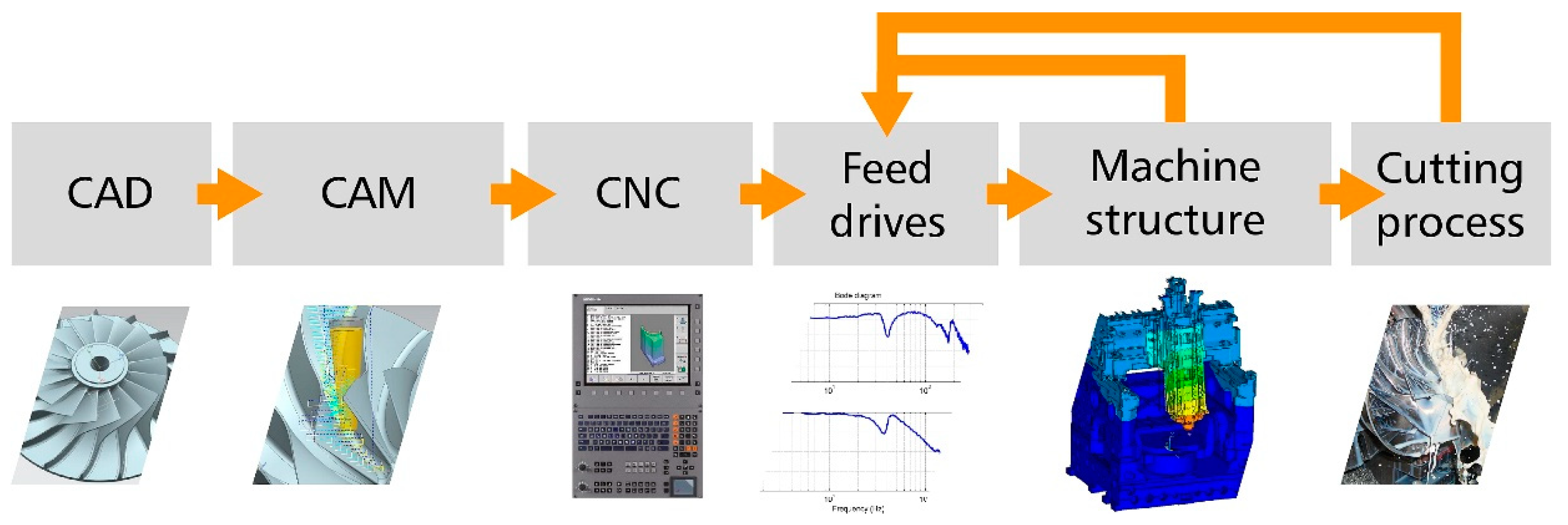
Several key factors influence the precision and surface quality of the final workpiece: the interpolator, the feed drive system, machine dynamics, and the machining process. The path from the CAD model of the part to the final workpiece can be represented by a chain of steps, as shown in Figure 1. Each step represents a potential source of error and, thus, affects the precision and surface quality of the machined part. The part model in the CAD SW has limited accuracy, especially for free-form surfaces. The CAM software then generates toolpaths based on the CAD model within a certain tolerance band around the nominal shape of the part in the form of CL data. By translating the CL data with a nonuniform point distribution using a postprocessor, a part program (NC program) with identical properties is generated. The conversion of the part program toolpaths from the geometric domain to the time domain is handled by the interpolator of the CNC machine control system. Its task is to achieve the smoothest, most accurate and time-saving tool speed profile along the NC program toolpath, typically represented by a sequence of linear segments and circular arcs. The main constraints of the interpolator are the user-defined tolerance band around the linear sections of the part program and the kinematic parameters defined by the machine manufacturer. The output of the interpolator is the position setpoint and the velocity profile setpoint, the quality of which is strongly influenced by several functionalities (look ahead, filtering, etc.) of the interpolator and their settings. This is the topic this paper focuses on, i.e., the effect of interpolator settings on the geometric quality, resp. surface quality, and accuracy of the output. The realization of tool movements according to the output of the interpolator is the task of the feed drive controller. The accuracy of the movements is determined by the dynamic properties of the controller, which are closely related to the dynamic properties of the feed drive components and the mechanical structure. Lastly, the accuracy and surface quality of the workpiece are influenced by the cutting process that generates the force load, its interaction with the feed drive controller, and the dynamic properties of the workpiece.

An interpolator is a component of the CNC system responsible for the transformation of the geometric NC toolpath into a vector of tool positions uniformly sampled in time. This vector needs to satisfy multiple conditions, such as acceleration and jerk limits and contour tolerance, all while attempting to keep the actual feedrate as close to the programmed feedrate as possible. It should also include a strategy for continuous transitions at the points of first- and second-order geometric discontinuities. CNC interpolation continues to be a popular research topic. Among the main subtopics of interpolation is the formulation of transition curves used to increase the order of geometric continuity of the original toolpath and the design of algorithms that plan the feedrate along a toolpath. Transition curves typically include circular arcs, B-spline curves [1,2,3], or clothoids [4,5,6]. The feedrate functions typically have the form of the trapezoid profile with piecewise constant jerk [7,8], or functions with continuous jerk [9,10,11,12,13,14]. The feedrate profile is typically formulated by continuation methods with bidirectional scanning [15,16], iterative methods [17], or global methods [18,19,20]. In recent years, the approach of finite impulse response (FIR) filtering to design feedrate profiles has gathered increasing attention. This approach does not require geometric smoothing of the toolpath by the introduction of transition curves and uses the composition of first-order filters instead. This makes controlling the contour error substantially more complex. In [21], however, this problem was solved by the authors for the case of three-axis machining. The authors modeled the corner blending behavior of NC systems using FIR filtering applied to a sequence of feedrate pulses, while providing analytical calculation of the minimal cornering feedrate that satisfies both the tolerance and the machining constraints. They demonstrated that the feedrate profile obtained in this way can predict the total cycle to high precision. In [22], the authors proposed a method of spline interpolation based on FIR filtering that does not require look-ahead and is capable of constraining the interpolation error. This result was expanded upon in [23], where the authors presented a method of real-time nonisometric dual-spline interpolation using FIR filtering.

The interpolator influences the precision and surface quality through the introduction of transition curves as well as by discrete sampling of the toolpath. While deviations caused by the introduction of transition curves (approximation error) can be controlled by a suitable choice of transition curve parameters [1], controlling deviations caused by discrete sampling of the interpolated toolpath is more complex and requires the introduction of additional constraints in interpolation algorithms. This type of error, commonly called the chord error, is defined as the Hausdorff distance of the interpolated toolpath from the required toolpath and is typically approximated via higher-order methods [24], due to the computational complexity of the exact evaluation. Several methods have been proposed to constrain the chord error during the interpolation process; see, e.g., [25,26,27].

Although the interpolation methods mentioned above are described explicitly in the literature, in practice, the CNC machine is equipped with an interpolator module provided by a commercial manufacturer (Siemens, Heidenhain, Fanuc, and others). The exact design of commercial interpolators is not known to the public, and the operator generally needs to rely on the recommendations provided in the technical manual as well as their personal experience.

However, it is difficult to accurately quantify the effect of interpolator parameter settings on the precision and quality of the final workpiece. Thus, the topic of interpolator parameter optimization has recently attracted the attention of several researchers. In [28], the limits of feedrate, acceleration, and jerk served as inputs to adaptive neuro-fuzzy inference systems with the aim of predicting the milling accuracy and surface quality (including the effects of the machine tool control loop and machined dynamics) based on results obtained on a rhombus testing toolpath. In [29], a CNC parameter tuning methodology was presented that focuses on three machining modes: high precision, high speed, and high quality. For each of these modes, the authors studied the effect of jerk and acceleration limits, corner velocity, the smoothing time constant, and radial acceleration on dynamic errors and machining time based on results obtained on several testing toolpaths, including the effects of the servo loop. However, the authors did not specify the interpolator manufacturer. In [30], an optimization algorithm for tuning CNC interpolation parameters based on a back-propagation neural network was presented. The algorithm aims to optimize contour errors, machining time, and corner vibrations simultaneously. The test data were obtained on a square testing toolpath and verified on a toolpath consisting of linear and circular segments. In [31], a genetic algorithm was applied to interpolator setting optimization with the aim to minimize the trajectory error without increasing the cycles. The authors used a simulation approach that combined the CNC interpolator output with a feed drive model to estimate the contour error. They did not, however, use a commercial interpolator as part of their model. Analogously to the previously mentioned papers, this paper presents a methodology focused on the evaluation of the effects of CNC interpolator settings on output quality and precision by formulating prediction models based on data obtained on a training toolpath and verifying the results on a verification toolpath. Unlike the above-mentioned paper, however, the presented method focuses on a specific commercial interpolator (namely, the iTNC530 by Heidenhain) and the effects of its parameter settings on toolpath quality and precision in corner neighborhoods without considering the effects of NC data quality, servo loop control, and machine dynamics. To this end, a novel method of estimating the quality of the toolpath in corner neighborhoods is introduced. This method primarily focuses on the variation in contour error as a function of the toolpath arclength. The overarching aim here is to use a simplified testing toolpath trajectory to model the dependence of quality and accuracy of the interpolator output on CNC parameter settings such as contour tolerance, limit frequency, and corner and axial jerk limits. As this model of interpolator behavior does not depend on the unique dynamical properties of the individual machine tool, it is applicable to any machine tool equipped with the same interpolator system. The presented results show that effective ranges exist for some of the investigated interpolator variables (most importantly, the corner jerk limits) that should be considered in the future design of CNC parameter optimization models that include the effects of the servo loop and machine dynamics.

To summarize, the main novelty of the presented research lies in the focus on toolpath quality and precision of the output of a specific commercial interpolator (excluding the effects of servo loop control and machine dynamics), leading to predictive models that are directly applicable to a wide range of machine tools. A novel method of toolpath quality evaluation based on the variation in contour error with respect to toolpath arclength is presented to this end.

This paper is organized as follows: The motivation for the research presented is presented at the beginning of Section 2. The general methodology is described in Section 2.1. The definitions of the test and validation toolpaths are given in Section 2.2 and Section 2.3, respectively. The contour error evaluation method is presented in Section 2.4 and the toolpath quality evaluation method is presented in Section 2.5. The interpolator parameters included in the test and their tested values are described in Section 2.6. Section 2.7 describes the data processing methods, while Section 2.8 includes details about experimental verification.

Section 3 focuses on the interpretation of the test results. The dependence of toolpath quality in corner neighborhoods on interpolator parameter settings is described in Section 3.1. Section 3.2 describes the dependence of maximal contour errors in corner neighborhoods on the interpolator parameter settings.

The discussion of the results presented, along with possible directions for future research, is presented in Section 4. The paper is concluded with Appendix A, in which the parameters of the presented regression models are given.

2. Materials and Methods

The purpose of this study was to provide a method to evaluate the effect of selection of interpolator parameters on the quality and precision of the (interpolated) toolpath for the Heidenhain iTNC 530 CNC system. Specifically, the effects of corner jerk settings on geometric precision and toolpath quality in corner neighborhoods were assessed in dependence on the selected limit frequency and desired machining tolerance.

This study focused primarily on the effects of the settings of the CNC parameter values of contour tolerance, limit frequency, and corner/axial jerk limits on the quality and accuracy of the toolpath output of the interpolator module (in contrast to the focus on the effects on the end result of the interpolator-control loop-dynamics-machining process chain, see [28,29,30]).

The reasons behind this choice can be summarized as follows: if the output of the interpolator itself does not satisfy the set criteria of toolpath quality or precision due to a suboptimal choice of CNC parameter values, the subsequent cumulative influence of the position control loop, machine dynamics, and machining process is likely to cause additional deterioration in both toolpath quality and precision. The quality of the interpolator output (as measured by the selected criteria) is thus a necessary (but not sufficient) prerequisite to achieve the desired level of workpiece quality.

Another compelling reason to study the influence of CNC parameter selection on the properties of the interpolator output is that the particular commercial implementation of the interpolator module is a common feature across a wide span of machine tools. Thus, information on the influence of CNC parameters on interpolator output quality can serve as a basis for subsequent optimization methods in a range of practical settings. This contrasts with the effect of position loop and machine dynamics, which can differ significantly based on the properties of the individual machine tool.

While the Heidenhain technical manual contains rules (both exact and rule-of-thumb) on parameter settings for many individual parameters, no such rule is provided for the axis-jerk limit at corners. The only advice given in the technical manual on this matter is the following [32], p. 833.

“In order to achieve the optimum results for your machine or application, test the various filter settings with a test part consisting of short, straight paths.”

This study shows that this parameter has a significant impact on surface quality and precision in corner neighborhoods and provides a possible methodology to quantify this influence.

2.1. Methodology

Two experimental toolpaths were used to evaluate the effects of interpolator settings on precision and toolpath quality in corner neighborhoods. The first toolpath consisted of a sequence of angles whose sizes formed a uniform sampling of the interval (110°, 170°) (see Section 2.2). The data obtained from this toolpath were used to quantify toolpath quality and formulate regression models characterizing the dependence of toolpath quality on the values of selected CNC parameters. The models were then verified on data obtained from the verification toolpath. The verification toolpath consisted of piecewise linear segments in the YZ plane separated by constant offsets along the X-axis (see Section 2.3). Both toolpaths were executed on an MCVL 1000 three-axis machining center as part of a full factorial experiment. During the machining process, the timestamp and position vectors generated by the interpolator were recorded. All subsequent data processing was realized with Matlab software.

Both toolpaths were specifically designed as simple piecewise linear paths. This was in line with the recommendation given for testing CNC parameter settings in the Heidenhain technical manual ([32], p. 833). This design also simplified the data evaluation process, as the NC code for such paths could be produced analytically and the exact locations and sizes of individual angles were known beforehand.

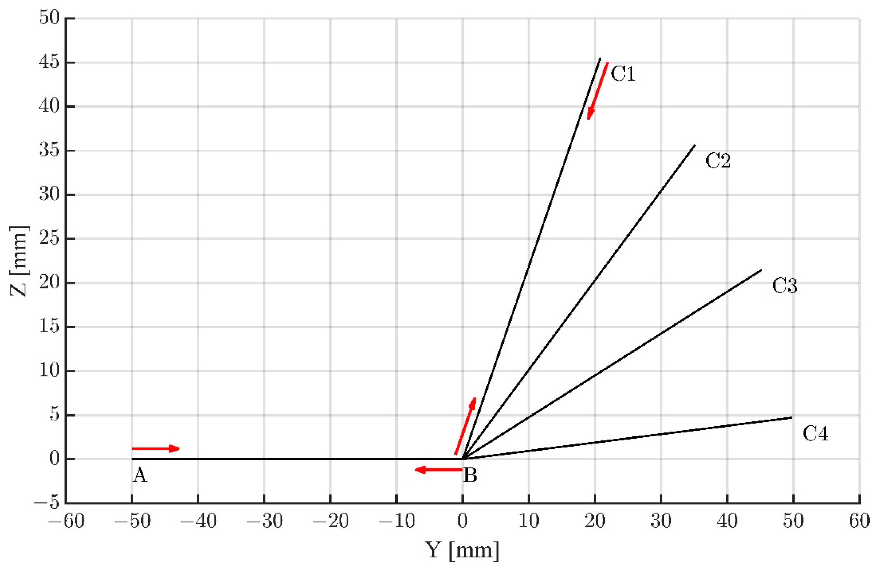
2.2. Definition of Test Toolpath “Fan”

The test toolpath (referred to as “Fan” in the following) consisted of a series of obtuse angles $AB{C}_i$ in the YZ working plane with arms of equal length arranged such that one of the angle arms was shared between all angles (see Figure 2). The path was traversed in the following way: the starting point lied on the nonvertex endpoint of the shared angle arm; the tool then traversed the first angle and returned via the same path back to the starting point to repeat the procedure by traversing the next angle (see Figure 2 for a schema of toolpath movement). Therefore, each angle that made up the toolpath was traversed in a forward and backward direction. The chosen angle sizes were 110°, 130°, 150°, and 170°. The ‘Fan’ toolpath describes the movement of the center point of a ball-end mill with a radius of 4 mm.

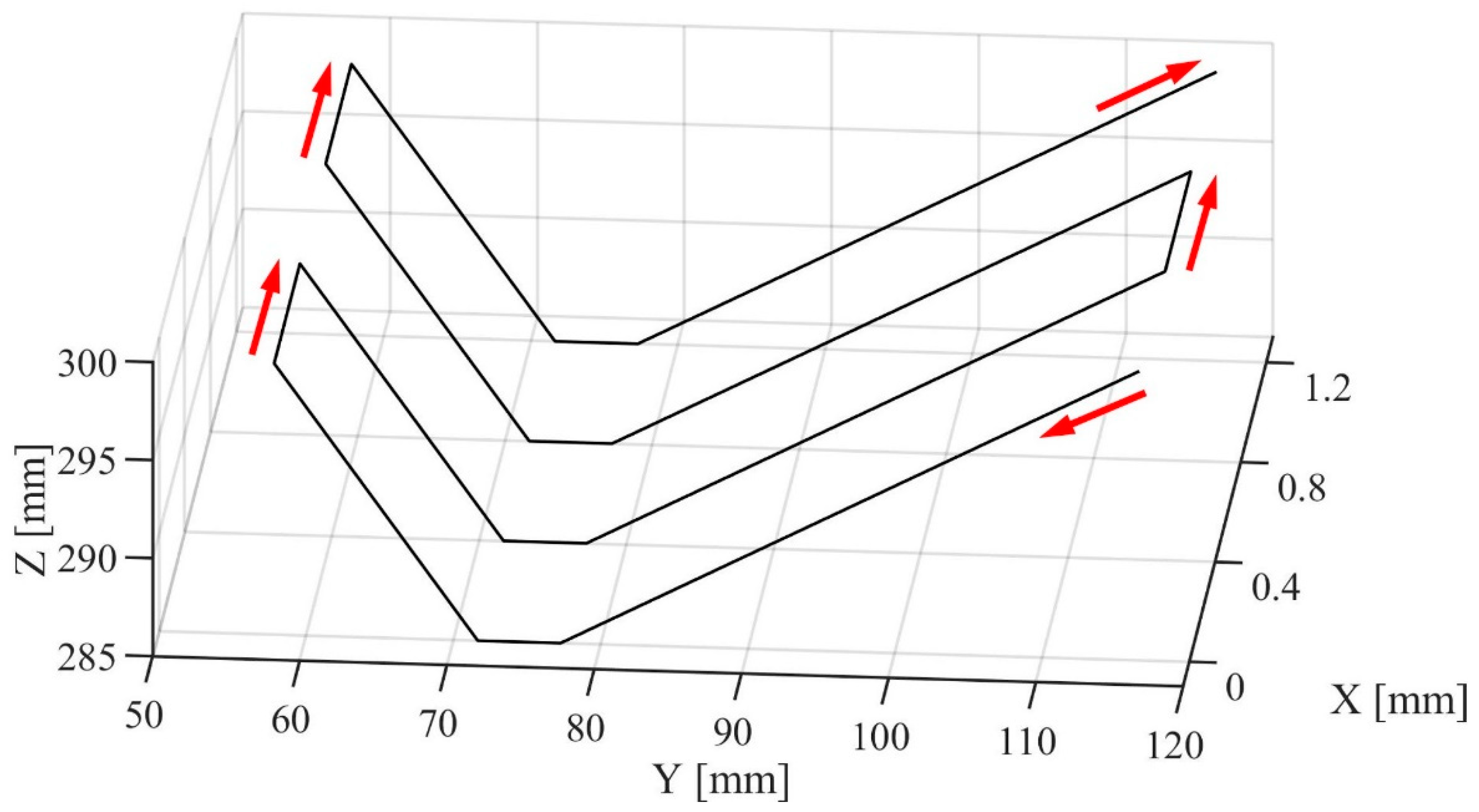
2.3. Definition of the Verification Toolpath “Valley”

The verification toolpath (referred to as “Valley” in the following) consisted of identical piecewise linear segments in the YZ working plane with adjacent segments connected by a linear block with constant offset in the X dimension (see Figure 3). This toolpath represents a typical example of the zig-zag machining strategy. The “Valley” toolpath describes the movement of the center point of a ball-end mill with a radius of 4 mm. The toolpath was programmed analytically (no CAM system was used).

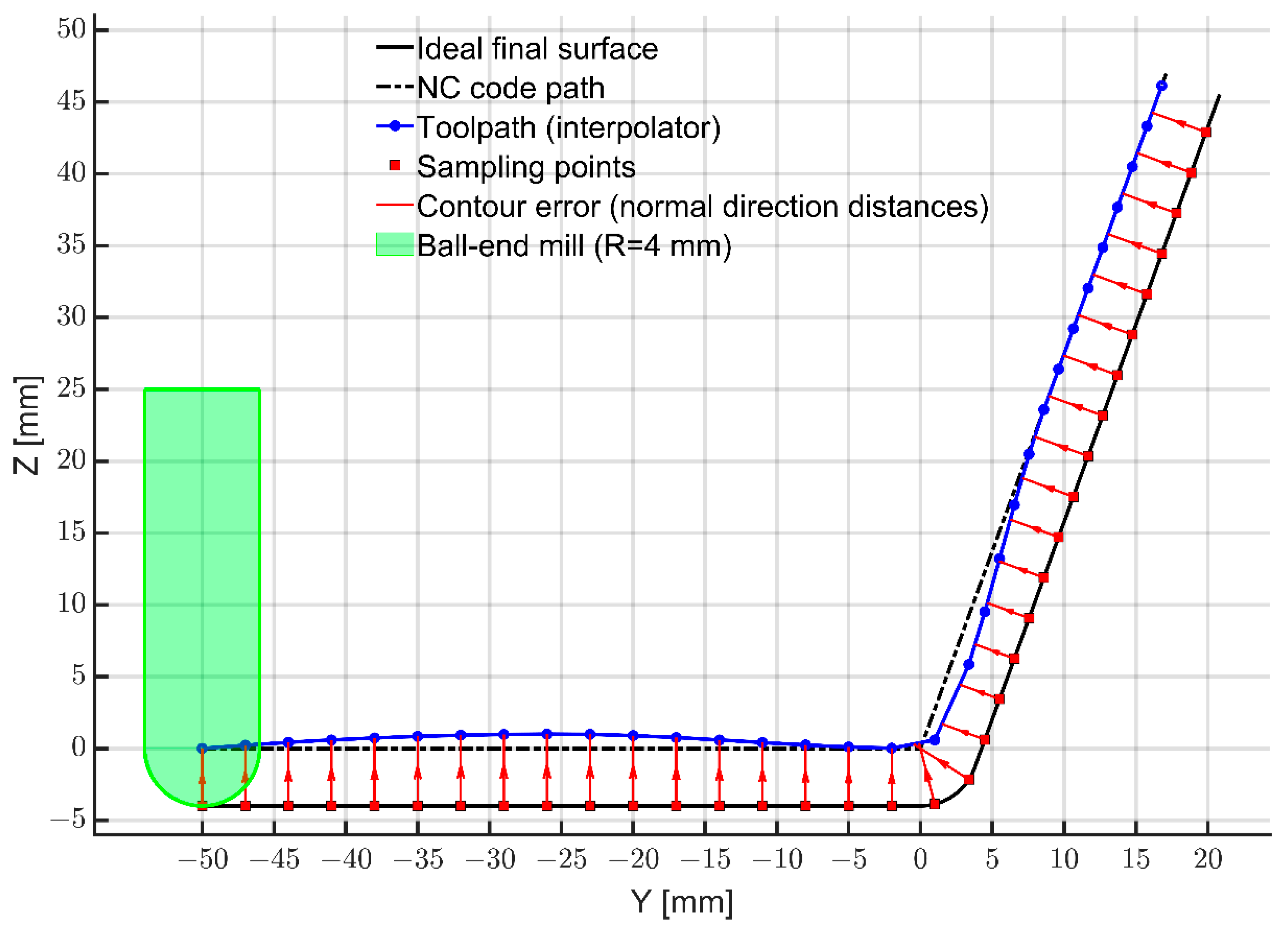
2.4. Contour Error Evaluation

To evaluate toolpath quality, a method of contour error evaluation is necessary. In the context of surface quality measurement, deviations from the ideal surface are typically evaluated using dedicated metrology equipment. However, these standard methods of surface quality evaluation are not applicable when evaluating deviations from the ideal surface based on position setpoint data obtained from the CNC interpolator. First, a physical workpiece cannot be machined based on the interpolator setpoint data only (i.e., without introducing the effects of machine dynamics and tool-workpiece force interaction). Therefore, the metrology equipment cannot be used. Second, the position datapoints are sampled with constant time frequency, potentially leading to a highly nonuniform distribution of these datapoints with respect to the toolpath length. Thus, the datapoints themselves cannot be used to evaluate surface quality according to standard ISO norms (as defined in ISO 4287 [33]).

To avoid these issues, the following contour error evaluation method was formulated and applied in the presented research. The geometric profile obtained as the cross-section of the required surface with the YZ work plane was first uniformly sampled with respect to its arclength; then, the outer normal direction vectors at the sampling points were evaluated. Given a specific toolpath processed by the interpolator, the locations of the tool center point were interpolated by a piecewise linear curve (in case of the Fan toolpath) or surface (in the case of the Valley toolpath). The contour error was then calculated at the sampling points as the (signed) distance to the interpolated curve/surface in the direction of the respective outer normal vectors. For a schematic of the contour error computation, see Figure 4. The Fan and Valley toolpaths were defined as trajectories of a center point of a spherical tool with a radius of 4 mm. Note that the contour error is represented as a function of arclength.

The presented definition of contour error evaluation was chosen for multiple reasons. First, by computing the contour error relative to the required surface, the effects of interpolator-introduced inaccuracies on the resulting surface geometry can be evaluated more directly compared to measuring deviations from the NC code toolpath. Second, by evaluating deviations at arclength-uniform sampling of the required surface-plane intersection, consistent estimates of the arclength-to-error function can be obtained across test results corresponding to different parameter value combinations.

2.5. Toolpath Quality Evaluation

In industrial practice, the structure of machined surfaces is prescribed in the production documentation, most often using the profile method and parameters defined by EN ISO 4287 [33]. Assessment of the structure of machined surfaces by means of measurements with touch (tip) instruments follows the rules and procedures standardized in EN ISO 4288 [34]. The direction of measurement is usually chosen perpendicular to the direction of the dominant texture or in the direction where the parameters to be evaluated take the highest values. The standards distinguish between nominal surface shape, shape deviation, waviness, and roughness (see Figure 5).

The surface quality parameters (Ra, Rz, etc.) are influenced by several factors, such as the cutting geometry of the tool and its state of wear, toolpath offsets in point machining, cutting conditions, the static and dynamic properties of the machine-tool-workpiece system, and tool and workpiece chatter. Next, surface parameters may locally deviate, usually near corners or transitions of surface curvature. From practical experience, it seems that the interpolator settings (such as the type of transition curve used at corners, contour tolerance, and (axial and corner) jerk limits) affect waviness rather than roughness. With a zig-zag machining strategy (which was applied when designing the “Valley” toolpath), this is usually most prominent in the dominant direction of the surface texture. Therefore, when looking for a suitable interpolator setting, it seems advantageous to approximate the waviness parameter, especially considering the sampling rate of interpolated data obtained from the control system, which generally does not allow the wavelengths corresponding to the roughness parameter to be captured.

Thus, the total variation coefficient (denoted as the TV coefficient in the following) was introduced in this study to evaluate the quality of the toolpath based on the output of the interpolator. The TV coefficient of a toolpath segment of total length $L$ is defined by Equation (1):

$$TV=\frac{1}{L}\underset{0}{\overset{L}{{\displaystyle \int }}}\left|\frac{\mathrm{d}{e}_c\left(s\right)}{\mathrm{d}s}\right|\mathrm{d}s$$

(1)

where $e_c\left(s\right)$ denotes the contour error (as described in Section 2.4.) at arclength $s$.

Mathematically, the TV coefficient expresses the total variation in the contour error with respect to the arclength of the toolpath, normalized by the total length of the toolpath. It is a unitless quantity. The contour error function $e_c\left(s\right)$ was defined as a piecewise-linear function interpolating the distance values obtained at sampling points of the required toolpath.

The TV coefficient is nonnegative and is zero exactly when the contour error is constant (not necessarily zero) along the whole segment. The TV coefficient reflects the dynamic behavior of the contour error along the respective toolpath (or its segment), thus serving as a measure of toolpath quality. For an illustrative example of the calculation of the TV parameter (1) and the effects of the oscillation of the deviation on its total value, see Figure 6.

It should be noted here that the use of the TV coefficient is justified when comparing cases in which the shape of the contour error function is similar up to scaling (such as in this study). The TV coefficient should not be used to compare cases for which the overall shape of the contour error function is substantially different, as different curve shapes can, in general, lead to the same value of the TV coefficient.

2.6. Selected Interpolator Parameters

As mentioned previously, the settings of the interpolator parameters have a major influence on the machining result. A single part program can be handled in many ways with varying degrees of preference for machining speed, accuracy, and surface smoothness. These objectives are influenced by parameters such as the type of position filter used (MP1200), contour tolerance (MP1202), cutoff frequency of the position filter (MP1210 to MP1218), and maximum allowable feed values (MP1010 to MP1020), as well as accelerations (MP1060 to MP1070) and jerk limits (MP1085 to MP1090) either on the path or in the individual axes. The parameters mentioned above modify the global properties of feedrate planning. Multiple parameters are also available that specify local behavior, such as interpolation jerk values (MP1230 to MP1243) at corners and curvature changes, the reduction in the contouring feedrate at the beginning of the contour elements (MP1205), the tolerance for changes in contour curvature (MP1223) and parameters specifying when and what transition to insert between two contour elements, and how to behave on it in terms of jerks (MP7680, bits 7, 8, and 9). These machine parameters must be optimally set in relation to the preferences of the machining result, and especially with regard to the current condition and mechanical properties of the machine tool structure.

The effects of multiple interpolator parameters on toolpath quality and precision in corner neighborhoods were investigated in this study. Specifically, these parameters were:

• Contour tolerance at machining feedrate (MP1202.0);
• Limit frequency for the advanced HSC filter (MP1213);
• Axis-specific jerk (MP1085.x);
• Axis-specific jerk at corners for the advanced HSC filter (MP1233.x).

The axis acceleration limit (MP1060.x) was initially included in the tests, but it was not found to have a significant effect on the quality, as evaluated by the TV coefficient (1), and was, therefore, excluded from the final tests.

The tested values for each of the investigated interpolator parameters are given in 1.

A full factorial experiment was performed based on the parameter values presented in

Table 1. Interpolator parameter values investigated in this study.

Parameter	Units	Values
MP1202.0 (contour tolerance)	$\mathrm{mm}$	0.02, 0.01, 0.1
MP1213 (limit frequency for the Advanced HSC filter)	Hz	10, 15, 20, 25, 30
MP1085.x (axis-specific jerk value)	$\mathrm{m}/{\mathrm{s}}^3$	10, 12.5, 15, 17.5, 20, 25, 30, 45, 65
MP1233.x (axis-specific corner jerk value)	$\mathrm{m}/{\mathrm{s}}^3$	1, 2.5, 5, 7.5, 10, 12.5, 15, 17.5, 20, 25, 30, 45, 65, 100

. The size and type of the machine used in the experiments were key in selecting the ranges of these parameters with the default settings of the machine manufacturer taken as reference.

To successfully capture the effect of the investigated parameters on the quality and precision of the interpolator output path, fixed settings were chosen for some interpolator parameters so that they did not bias the test result. For example, the path limitations on acceleration and jerk were removed so that only the settings of the individual axes were limiting and the errors were easier to observe. The same acceleration and jerk limits were always chosen in all axes so that the boundary conditions in the interpolation calculation were comparable. Acceleration values were fixed at the value of the weaker of the tested axes so that the mechanical components of the machine, which were designed by the manufacturer for a certain acceleration, could not be damaged. The Advanced HSC position filter was chosen for the tests as it allows for a good compromise between the machining speed and the quality of the machined surface. The Heidenhain technical manual offers the following comment on the HSC filters (standard and advanced) ([32], p. 829):

“The speed advantage of both HSC filters is especially large for circular contours. However, you must consider slight overshoots at corners and curvature transitions that are within the given tolerances.”

Such overshoots are indeed present in corners. However, contrary to the above comment, these overshoots can significantly exceed the given tolerances, as shown in Section 3.2.

The parameters of the interpolation jerk limits at curvature changes (MP1243.x) and the parameter specifying the consideration of contour tolerance at curvature changes (MP1233) were fixed at the manufacturer’s default values as they do not influence the interpolator output for piecewise linear NC codes. The settings regarding the characteristics of transitions between two contour elements were also fixed. Specifically, the spline transition curve ($bit10=1$ in parameter MP7680) was applied. Although this selection leads to slower machining times (in comparison with the rounding arc transition curve), the spline produces additional jerk reduction by introducing a G1 transition instead of G0. A high feed rate of 10,000 mm/min was chosen for the tests to investigate the behavior of the interpolator under extreme conditions. In practice, such conditions can be applied in light alloy machining, and high-speed or high-feed machining.

2.7. Data Processing

For the ‘Fan’ test toolpath, the TV coefficients were evaluated for each angle of the path separately and then these results were averaged to obtain the final values for the specific combination of test parameters.

In the case of the Valley verification path, the TV index was computed separately for each segment in the YZ plane with a constant X-axis value. The mean of these values was then reported as the final TV index for the specific parameter combination. It should be noted here that the variation in the TV values between the segments was insignificant. This was confirmed by comparing the output of the interpolator in neighboring segments, i.e., segments that differ in their sense of direction (see Figure 3), which were found to be practically identical. In other words, the size and distribution of deviations from the ideal surface caused by the interpolator did not depend on the sense of direction of the toolpath.

The value of the maximum contour deviation as a measure of precision was evaluated separately for each individual angle size of the Fan toolpath. For the Valley toolpath, the maximal contour error value measured along the entire toolpath was reported.

2.8. Obtaining the CNC Position Setpoint Data

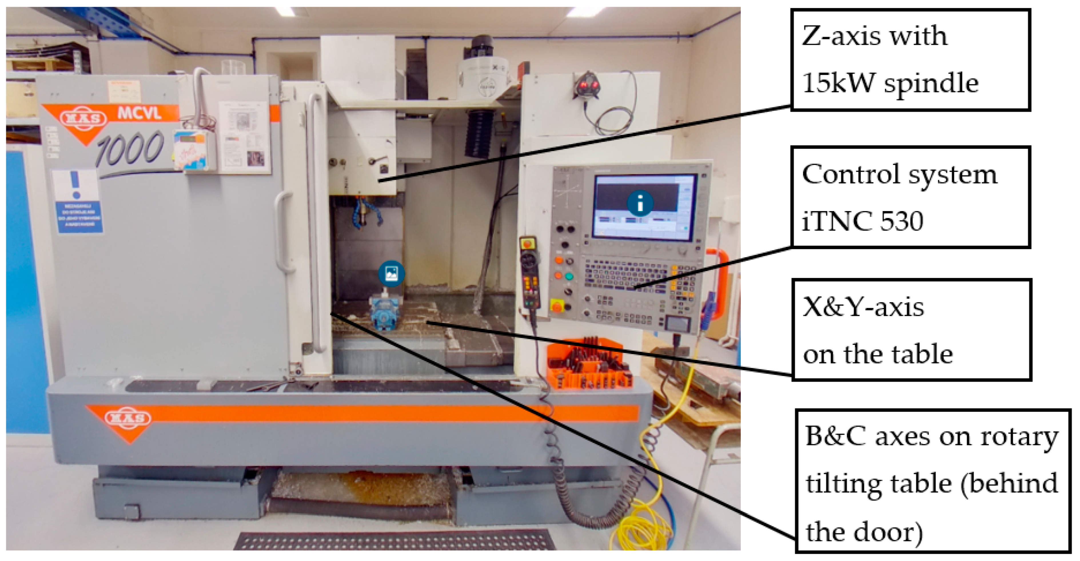
Tests of the effect of the interpolator settings were performed on a MCVL 1000 milling machine produced by Kovosvit MAS with a Heidenhain iTNC 530 control system (see Figure 7). The MCVL 1000 is a standard three-axis vertical machine tool with a 15 kW spindle supplemented by a tilting rotary table (axes B and C).

Two prepared part programs with a 2D path were processed in the YZ plane in “air cut” mode. For each of them, more than 1800 measurements were taken at unique interpolator settings. This number was only possible because of the automation of the measurements and the bulk processing of the acquired data. The design of the full-factorial experiment allowed the influence of all possible combinations of the considered machine parameter settings to be verified.

The individual steps of the procedure of changing the machine parameter settings, i.e., start of the recording of the time histories in the individual machine axes, execution of the NC program, and termination and saving of the recording, were carried out completely autonomously without the need for intervention of the machine operator.

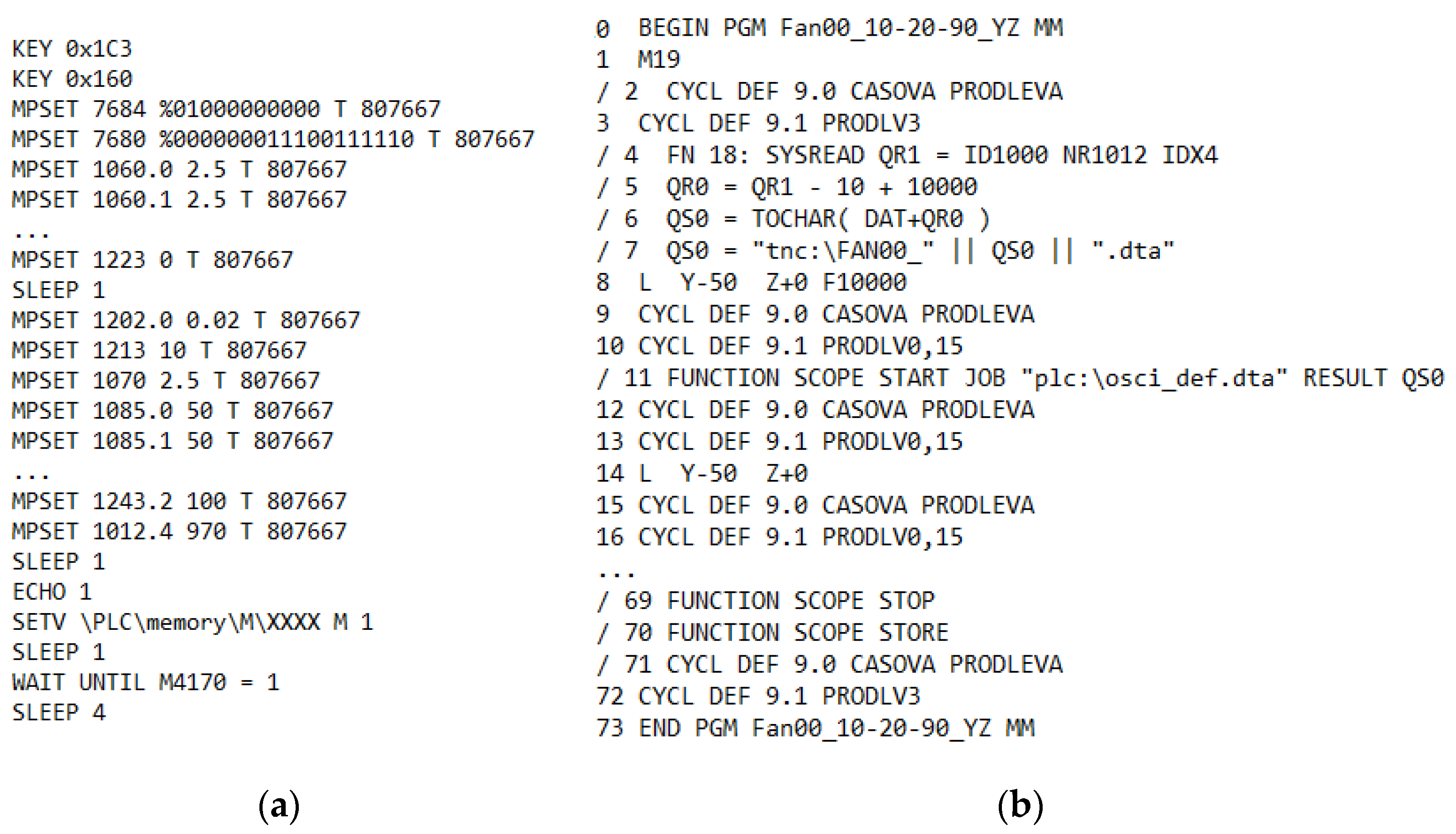
The use of the Heidenhain TNCcmd tool, which enables remote control of the iTNC control system from an external computer using specific commands, was essential in this regard. For example, it is possible to temporarily change the value of a given machine parameter in the operating memory of the control system. Similarly, it is possible to change the value of the bit indicating the start of a program in memory and wait until the part program is executed. TNCcmd allows for processing a series of consecutive commands stored in a text file with the extension “tnccmd”. This file was created in the MATLAB environment. An example sequence for executing one test is shown in Figure 8a. First, the parameter values were set according to the specific dataset using the MPSET command. This was followed by the execution of the NC program using the SETV command (the value of the specific marker is not disclosed, for security reasons) and waiting until the program was executed using the WAIT UNTIL command. The sequence was padded with delays (SLEEP command) so that the control system had sufficient time to execute all commands.

For each of the interpolating axes (Y and Z), the time histories of the output trajectories of the interpolator were recorded using the internal oscilloscope (OSCI) of the iTNC control system. The recording was automatically started, terminated, and saved, with a name containing the measurement serial number, using commands directly from the part program (see Figure 8b).

The experiment set-up in this fashion was then executed by loading the appropriate part program on the machine in automatic mode and setting the feedrate override displacement values to 100%. The connection to the machine was then activated (using its IP address) from the TNCcmd console running on an external PC. Subsequently, a batch file was run, which contained a sequence of commands to execute a series of tests. Records from the internal oscilloscope were continuously stored in a user-accessible section of the machine’s storage, and, after all tests were completed, these records were downloaded from the machine for bulk evaluation.

3. Results

This chapter summarizes the results obtained by the analysis of experimental data. Specifically, the dependence of the TV parameter on corner jerk, contour tolerance, and limit frequency is described in Section 3.1. and the dependence of maximal contour error on angle size, corner jerk, contour tolerance, and limit frequency is described in Section 3.2. In all cases, the prediction models were established on the basis of the results obtained on the testing toolpath “Fan” and later verified on the “Valley” toolpath.

3.1. Parameter TV—Dependence on CNC Parameter Settings

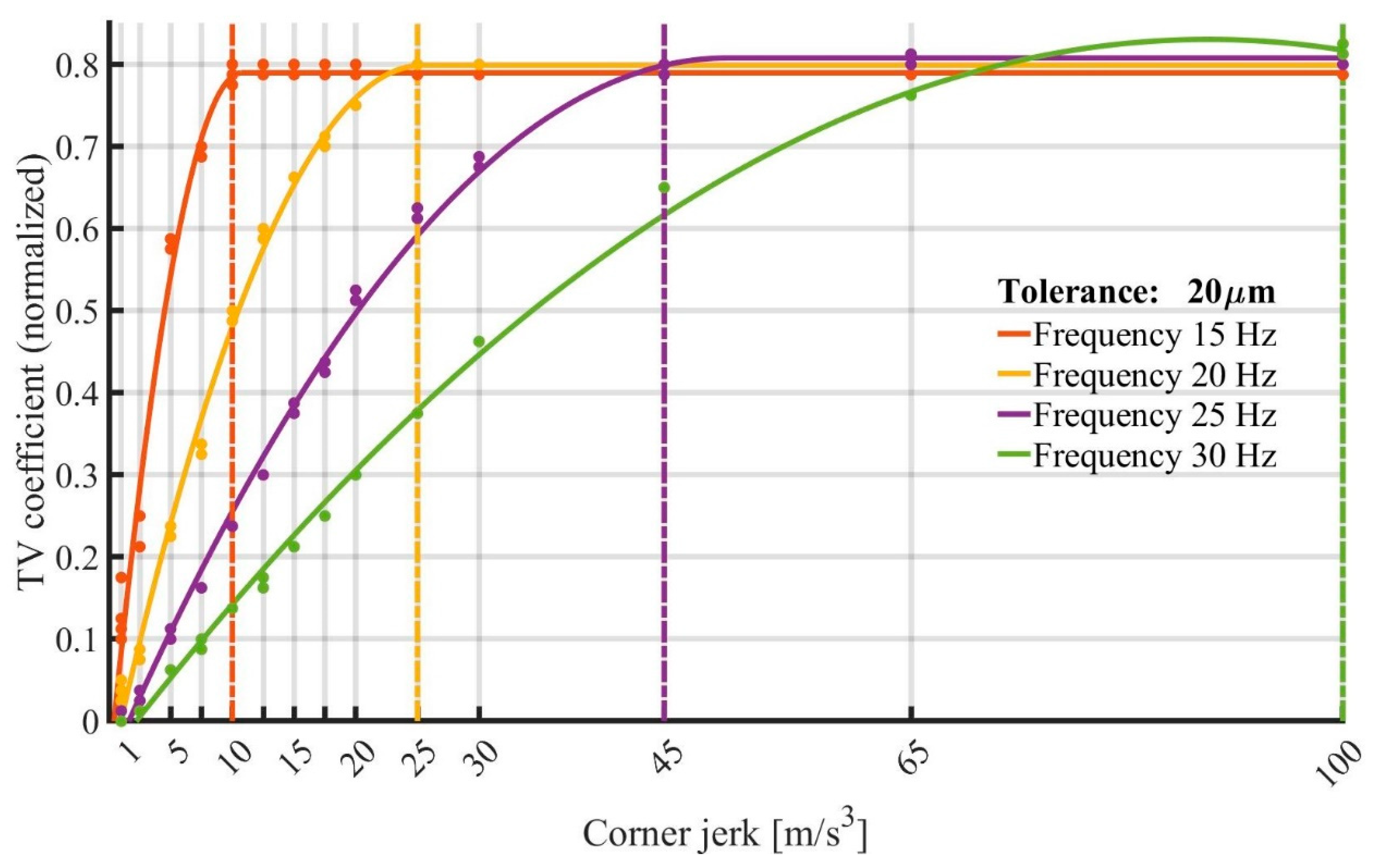
The TV parameter was found to depend on four of the investigated interpolator parameters: contour tolerance, limit frequency, axis-specific jerk, and axis-specific jerk at corners.

Two types of dependence of the TV parameter were distinguished on the basis of the experiments performed. For high contour tolerances and/or high values of limit frequency, the TV coefficient was found to depend only on the corner jerk limit and the dependence could be adequately described by a quadratic model (these situations correspond to 80% of the studied cases). In contrast, when both low contour tolerance and low limit frequency were selected, the TV coefficient was found to depend approximately quadratically on both the axis-specific jerk and the corner jerk limit.

In either of the two cases, the choice of limit frequency and contour error values affected the range of corner jerk limit values that had a measurable effect on the TV coefficient. In other words, the lower the limit frequency and contour tolerance, the lower the corner jerk limit threshold, after which an additional increase in the corner jerk limit did not influence the TV parameter. The values of these corner jerk thresholds depending on contour tolerance and limit frequency are presented in

Table 2. Corner jerk threshold values ($\mathrm{m}/{\mathrm{s}}^3$) with respect to specific combinations of the contour tolerance limit (horizontal) and the limit frequency (vertical). Increasing corner jerk beyond the threshold values does not affect the value of the TV coefficient. The threshold values presented with * denote combinations for which a significant dependence on the axis jerk limit was found (see the commentary in the second half of this section). The values are based on the “Fan” toolpath results.

Corner Jerk $(\mathbf{m}/{\mathbf{s}}^3)$ Threshold Values with Respect to Contour Tolerance Limit (mm) and Limit Frequency (Hz)
Contour Tolerance (mm)\Limit Frequency (Hz)	0.01	0.02	0.1
10	2.5 *	5 *	15
15	5 *	10	45
20	12.5	25	100
25	25	45	100
30	45	100	100

.

For each combination of contour error and frequency limit, the corresponding TV values from each individual data source (Fan and Valley toolpaths) were min-max-normalized for the purposes of comparison. Quadratic regression models were then fitted to the Fan toolpath interpolator data and verified on the Valley toolpath data.

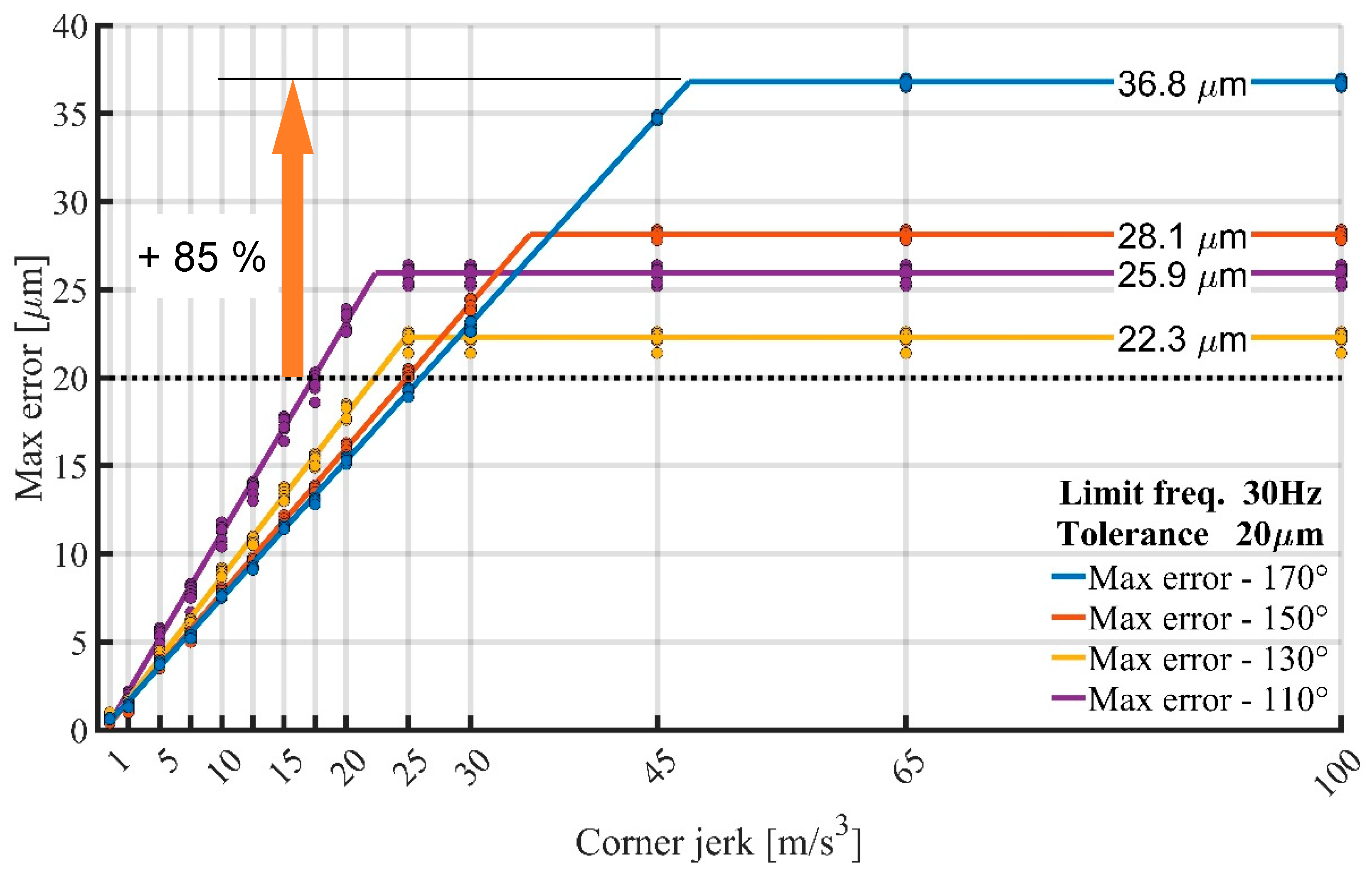
The results show that the regression models explain a large percentage of the predicted variance (R-Sq. (adj.)$\ge 0.97$) and the models fitted on the Fan toolpath interpolator data generalize well ($RMSE\le 0.068$) to Valley data. Figure 9 presents a comparison of the models obtained for a contour accuracy of 20 µm and varying values of limit frequency. For detailed information on the regression models corresponding to high contour tolerance/high limit frequency, see Appendix A,

Table A2. Parameters of regression models describing the dependence of the TV coefficient on the corner jerk limit (denoted by $J_c$), results for contour tolerance of 10 µm. Postfixes L and U denote the lower and upper limits of the 95% confidence intervals, respectively.

Contour tolerance (mm)	0.01	0.01	0.01
Limit frequency (Hz)	20	25	30
Corner jerk threshold (m/s3)	12.5	25	45
Intercept	7.82 × 10−1	1.25 × 10−1	−7.77 × 10−2
Intercept_L	6.88 × 10−1	1.14 × 10−1	−9.39 × 10−2
Intercept_U	8.77 × 10−1	1.36 × 10−1	−6.16 × 10−2
Jc	9.24 × 10−2	1.63 × 10−1	1.57 × 10−1
Jc L	4.30 × 10−2	1.59 × 10−1	1.51 × 10−1
Jc U	1.42 × 10−1	1.66 × 10−1	1.63 × 10−1
Jc2	0.00 × 100	0.00 × 100	−6.08 × 10−3
Jc2 L	0.00 × 100	0.00 × 100	−6.51 × 10−3
Jc2 U	0.00 × 100	0.00 × 100	−5.64 × 10−3
Adj. RSquare	4.96 × 10−1	9.79 × 10−1	9.90 × 10−1
RMSE	7.00 × 10−2	4.05 × 10−2	3.23 × 10−2
RMSE Valley (validation)	3.38 × 10−2	3.14 × 10−2	3.44 × 10−2

(contour tolerance 10 µm),

Table A3. Parameters of regression models describing the dependence of the TV coefficient on the corner jerk limit (denoted by $J_c$ ), results for contour tolerance of 20 µm. Postfixes L and U denote the lower and upper limits of the 95% confidence intervals, respectively.

Contour tolerance (mm)	0.02	0.02	0.02	0.02
Limit frequency (Hz)	15	20	25	30
Corner jerk threshold [m/s3]	10	25	45	100
Intercept	−7.96 × 10−2	−7.78 × 10−2	−6.62 × 10−2	−5.18 × 10−2
Intercept_L	−1.28 × 10−1	−9.05 × 10−2	−7.66 × 10−2	−5.81 × 10−2
Intercept_U	−3.10 × 10−2	−6.51 × 10−2	−5.58 × 10−2	−4.54 × 10−2
Jc	1.92 × 10−1	8.21 × 10−2	4.18 × 10−2	2.38 × 10−2
Jc L	1.70 × 10−1	7.98 × 10−2	4.06 × 10−2	2.33 × 10−2
Jc U	2.14 × 10−1	8.45 × 10−2	4.29 × 10−2	2.42 × 10−2
Jc2	−8.89 × 10−3	−1.61 × 10−3	−4.17 × 10−4	−1.33 × 10−4
Jc2 L	−1.09 × 10−2	−1.70 × 10−3	−4.43 × 10−4	−1.38 × 10−4
Jc2 U	−6.92 × 10−3	−1.52 × 10−3	−3.91 × 10−4	−1.29 × 10−4
Adj. RSquare	9.77 × 10−1	9.96 × 10−1	9.95 × 10−1	9.97 × 10−1
RMSE	4.98 × 10−2	2.19 × 10−2	2.22 × 10−2	1.79 × 10−2
RMSE Valley (validation)	4.33 × 10−2	2.65 × 10−2	2.95 × 10−2	2.55 × 10−2

(contour tolerance 20 µm), and

Table A4. Parameters of regression models that describe the dependence of the TV coefficient on the corner jerk limit (denoted by $J_c$), results for contour tolerance of 100 µm. Postfixes L and U denote the lower and upper limits of the 95% confidence intervals, respectively.

Contour tolerance (mm)	0.1	0.1	0.1	0.1	0.1
Limit frequency (Hz)	10	15	20	25	30
Corner jerk threshold (m/s3)	15	45	100	100	100
Intercept	−2.93 × 10−2	−5.68 × 10−2	−1.98 × 10−2	−8.88 × 10−3	−6.51 × 10−3
Intercept_L	−4.31 × 10−2	−6.98 × 10−2	−2.33 × 10−2	−9.55 × 10−3	−7.04 × 10−3
Intercept_U	−1.55 × 10−2	−4.38 × 10−2	−1.63 × 10−2	−8.20 × 10−3	−5.97 × 10−3
Jc	1.39 × 10−1	4.44 × 10−2	1.60 × 10−2	7.24 × 10−3	4.25 × 10−3
Jc L	1.35 × 10−1	4.29 × 10−2	1.57 × 10−2	7.20 × 10−3	4.21 × 10−3
Jc U	1.44 × 10−1	4.58 × 10−2	1.62 × 10−2	7.29 × 10−3	4.28 × 10−3
Jc2	−4.39 × 10−3	−4.56 × 10−4	−6.37 × 10−5	1.10 × 10−6	1.40 × 10−6
Jc2 L	−4.65 × 10−3	−4.88 × 10−4	−6.61 × 10−5	7.00 × 10−7	1.00 × 10−6
Jc2 U	−4.12 × 10−3	−4.24 × 10−4	−6.14 × 10−5	1.60 × 10−6	1.70 × 10−6
Adj. RSquare	9.92 × 10−1	9.93 × 10−1	9.93 × 10−1	1.00 × 100	1.00 × 100
RMSE	3.24 × 10−2	2.71 × 10−2	2.47 × 10−2	2.00 × 10−3	1.50 × 10−3
RMSE Valley (validation)	6.87 × 10−2	6.00 × 10−2	5.04 × 10−2	3.48 × 10−2	1.98 × 10−2

(contour tolerance 100 µm).

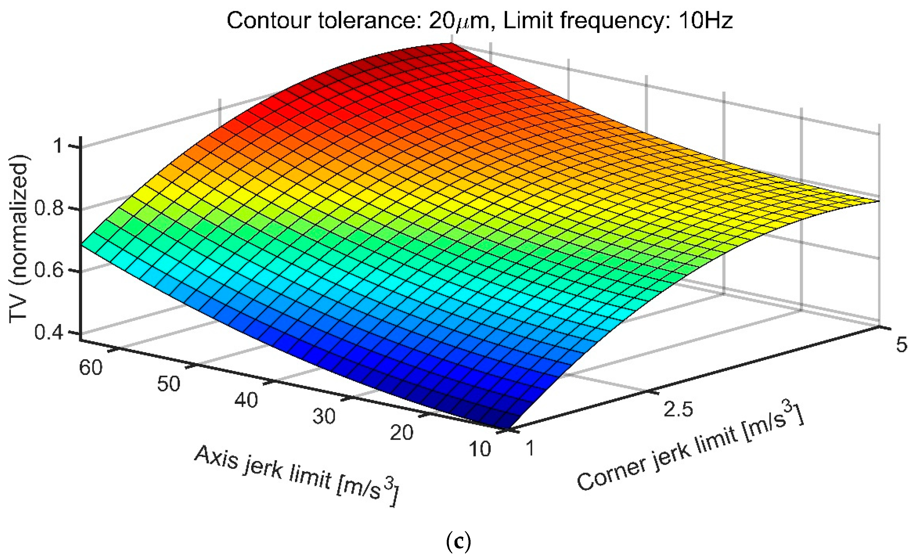
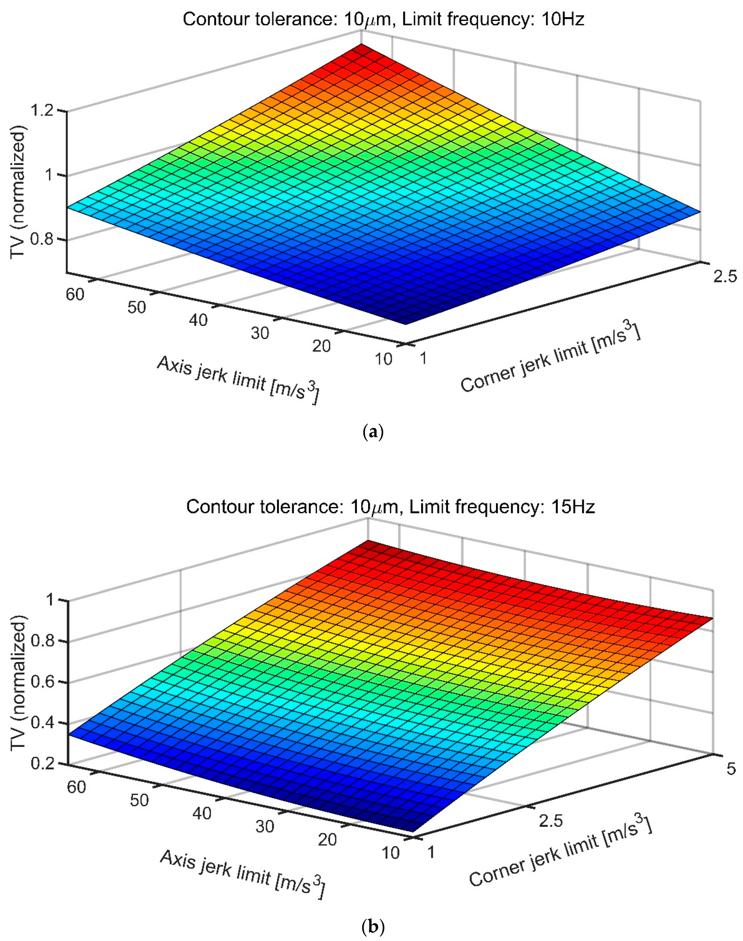
The case of low contour tolerance limit and low frequency threshold (combinations denoted by * in Table 2) was slightly different. In these cases, the TV coefficient depended not only on the corner jerk limit, but also on the axis jerk limit. The dependence was quadratic and increasing with respect to both parameters. In other words, both the increase in the corner jerk limit and the increase in the axial jerk limit led to an increase in the TV parameter. The dependence could be adequately described by a model of the form of Equation (2)

$$TV~a_0+a_1{J}_c+a_2{J}_c{J}_a+a_3{J}_a^2+a_4{J}_c^2$$

(2)

where $J_a, J_c$ denote the values of the axial jerk limit and the corner jerk limit, respectively. Note that the linear term in $J_a$ is omitted in (2), as it did not show itself to be statistically significant in the performed tests.

As in the case mentioned above, the regression models explain a large percentage of the predicted variance (R-Sq. (adj.)$\ge 0.87$) and the models fitted on the test toolpath interpolator data generalize well ($RMSE\le 0.06$) to Valley toolpath data. For the regression model surfaces, see Figure 10. For detailed information on the corresponding regression models, see Appendix A,

Table A1. Parameters of the multiregression models describing the dependence of the TV coefficient on the corner jerk limit (denoted by $J_c$) and the axis jerk limit (denoted by $J_a$). Results for combinations of low contour tolerance and low limit frequency. Postfixes L and U denote the lower and upper limits of the 95% confidence intervals, respectively.

Contour tolerance (mm)	0.01	0.01	0.02
Limit frequency (Hz)	10	15	10
Corner jerk threshold (m/s3)	2.5	5	5
Intercept	7.27 × 10−1	3.92 × 10−2	9.29 × 10−2
Intercept L	6.89 × 10−1	2.40 × 10−2	7.48 × 10−2
Intercept U	7.65 × 10−1	5.45 × 10−2	1.11 × 10−1
Jc	0.00 × 100	1.94 × 10−1	3.20 × 10−1
Jc L	0.00 × 100	1.81 × 10−1	3.05 × 10−1
Jc U	0.00 × 100	2.06 × 10−1	3.34 × 10−1
JcJa	1.92 × 10−3	−4.35 × 10−4	−3.96 × 10−4
JcJa L	4.83 × 10−4	−5.49 × 10−4	−5.30 × 10−4
JcJa U	3.36 × 10−3	−3.21 × 10−4	−2.61 × 10−4
Jc2	1.28 × 10−2	−4.97 × 10−3	−3.58 × 10−2
Jc2 L	−5.64 × 10−4	−6.89 × 10−3	−3.80 × 10−2
Jc2 U	2.62 × 10−2	−3.05 × 10−3	−3.35 × 10−2
Ja2	9.10 × 10−6	3.52 × 10−5	7.98 × 10−5
Ja2 L	−2.72 × 10−5	3.03 × 10−5	7.40 × 10−5
Ja2 U	4.53 × 10−5	4.02 × 10−5	8.57 × 10−5
Adj.RSquare	8.72 × 10−1	9.99 × 10−1	9.97 × 10−1
RMSE	3.99 × 10−2	8.40 × 10−3	1.00 × 10−2
RMSE Valley (validation)	6.04 × 10−2	4.74 × 10−2	2.83 × 10−2

.

In practice, low-limit frequency settings are typical for large machine tools or budget machine tools with lower-quality mechanical components. As can be seen from the results in Figure 10, if a low-contour-error oscillation is required in corner neighborhoods in the case of low-contour-tolerance and low-limit-frequency settings, the corner jerk limit should be kept to minimal values (~1 $\mathrm{m}/{\mathrm{s}}^3$) and axial jerk limits should ideally not exceed 30 $\mathrm{m}/{\mathrm{s}}^3$.

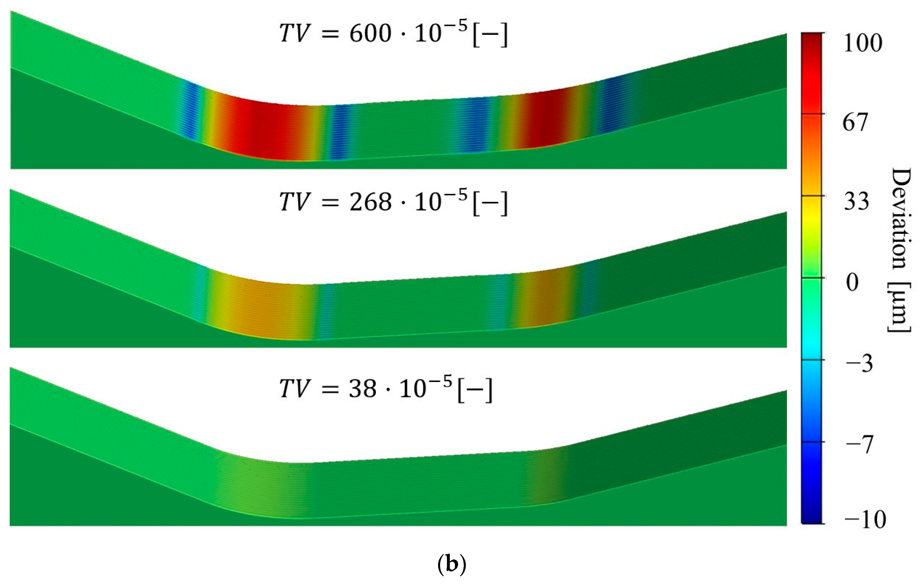
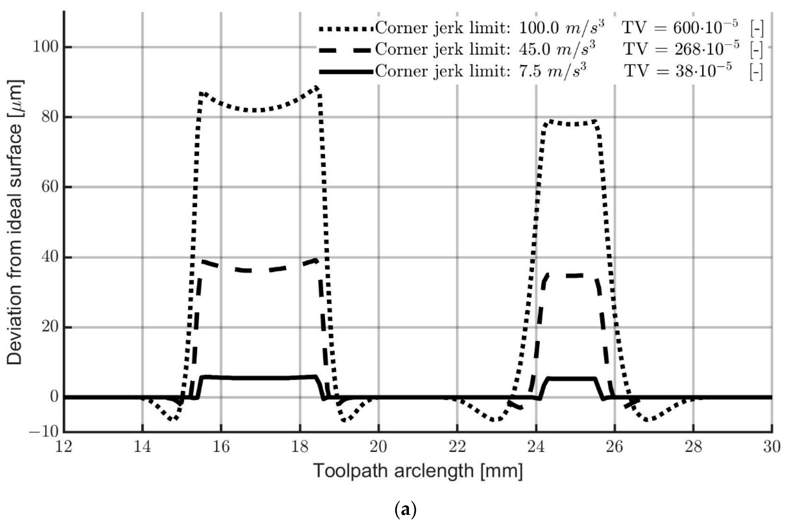
An illustrative demonstration of the effect of corner jerk limit settings on the distribution of toolpath deviations in corner neighborhoods and its effect on the TV parameter is presented in Figure 11.

3.2. Maximal Contour Error—Dependence on CNC Parameters

Another parameter investigated was the maximum contour error. It was measured as the maximum absolute value of the contour error relative to the ideal final surface (see Section 2.4.). It should be noted here that the maximal contour error was attained in corner neighborhoods as a rule. This is not surprising, as the iTNC interpolator is able to interpolate line segments exactly. Therefore, the only areas where significant contour deviations can occur are precisely the corner neighborhoods (see Figure 11).

The maximal contour error does, in general, depend on the parameters of contour tolerance, limit frequency, corner jerk, and angle size. Interestingly, the axial jerk limits did not affect the maximal contour error values. When both values of contour tolerance and limit frequency are fixed, the dependence of maximal error on corner jerk for individual angle sizes has the following character: for lower values (up to a certain threshold) of the corner jerk, the dependence is linear, while for higher values of corner jerk, the dependence is constant. Thus, given values of contour tolerance, limit frequency, and angle size, there exists a corner jerk threshold value such that an additional increase in the corner jerk parameter beyond this value does not have an additional effect on the maximal contour error. For an example of this type of dependence, see Figure 12.

Based on the results obtained from the tests performed on the Fan toolpath, the maximal contour error can significantly exceed the prescribed contour tolerance. In fact, the contour tolerance limit can be exceeded by as much as 85% (see Figure 12). Thus, based on the regression models obtained from the experimental results, the maximal corner jerk values for which the contour tolerance is satisfied for all measured angle sizes (depending on the limit frequency and contour error settings) were calculated. These results are summarized in

Table 3. Dependence of maximal contour error on corner jerk values. The presented corner jerk values ($\mathrm{m}/{\mathrm{s}}^3$) represent maximal values for which the contour tolerance was not exceeded for any of the tested angle sizes. The values were obtained by interpolation/extrapolation of the respective regression models formulated on the basis of “Fan” toolpath data and rounded to one decimal place.

Maximal Contour Error: Maximal Values of Corner Jerk $\left(\mathbf{m}/{\mathbf{s}}^3\right)$ for Which Contour Tolerances Are Satisfied
Contour Tolerance (mm)\Limit Frequency (Hz)	0.01	0.02	0.1
10	0.8	2.4	7.3
15	3.6	4.5	19.3
20	5.9	9.8	43.8
25	9.5	17.4	86.7
30	14.9	28.3	138.4

.

The results obtained from the performed tests show that the overshoots at corners can exceed the prescribed tolerances significantly depending on the limit frequency and the value of the corner jerk limit.

As can be seen in Table 3, the range of corner jerk values for which the tolerance limit is satisfied increases with both the contour tolerance limit and the frequency limit. The impact of angle size on the dependence of maximal error on corner jerk is not readily discernible. It can be assumed that this influence is a result of the interaction between the selected filter type, the limit frequency, and the angle size. This interaction is difficult to model because the technical details of the iTNC interpolator implementation are not known.

Despite this difficulty, the results show that practical information about the behavior of the interpolator system can still be obtained. The corner jerk limits presented in Table 3 refer to the worst-case scenarios and can thus be applied to general toolpaths to ensure that the programmed contour tolerance limit is satisfied at corners.

This approach was also verified on the Valley toolpath. The results agreed with the predictions (i.e., contour tolerance was satisfied for tested corner jerk values below the respective thresholds and maximal errors exceeded contour tolerance for corner jerk values above the thresholds).

4. Discussion

This study investigated the effects of CNC parameter settings (contour tolerance, limit frequency, and axial and corner jerk limits) on the quality and accuracy of the interpolator output in corner neighborhoods. The results obtained on the basis of a full factorial test performed on a simplified testing toolpath consisting of linear blocks were used to build regression models, which were then verified on a general piecewise linear toolpath.

The results of this study show that excessively high corner jerk limits can lead to a significant overshoot of the programmed path tolerance (by as much as 85% in some cases) in corner neighborhoods. This study, therefore, presents the maximum values of corner jerk limits for which the programmed path tolerance is maintained, independent of the magnitude of the angle between two adjacent linear blocks. The values of these jerk limits depend on the chosen tolerance limit and the value of the limit frequency of the interpolator.

In addition to the toolpath accuracy, the variation in the deviation from the ideal surface along the toolpath has a significant effect on the quality of the final workpiece. This study presents a method to quantify this oscillation of the deviation in the toolpath from the ideal surface and, thus, evaluate the geometric quality of the interpolator output in corner neighborhoods. The results of the tests performed show that the quality of the interpolator output around corners is primarily dependent on the choice of the tolerance limit and the interpolator limit frequency, and secondarily on the choice of the corner and axial jerk limits. Therefore, for successful quality control, it is first necessary to specify the desired tolerance and limit frequency of the interpolator and then control the resulting quality of the interpolator output by the choice of the jerk limits. In practice, this requirement is not limiting, as the parameters of the tolerance limit and the limit frequency result from the overall accuracy requirements (tolerance limit) or the dynamic characteristics of the machine (in the case of the limit frequency) and are, thus, known in advance for the application. The results obtained show that, once these parameters are fixed, the choice of the corner and axial jerk limits can effectively reduce the rate of deviation oscillation in corner neighborhoods.

Previous studies investigating the topic of interpolator parameter optimization differ from the present study in several important ways. In addition to the influence of the interpolator itself, previous studies simultaneously include the influence of feed drive control and machine dynamics [28,29,30,31]. These models are certainly more comprehensive, but at the same time, their results are only valid for a specific machine tool, and to apply them to a machine with different mechanical and kinematic properties, the demanding optimization process must be repeated. In contrast, the results of the presented study are directly applicable to any machine tool equipped with the same interpolator module, as the consistent behavior of the interpolator is guaranteed by the manufacturer.

The practical application of the presented results lies in controlling toolpath quality and precision at the interpolator level. Thus, the machine tool operator can be certain that the potentially observed lack of precision or surface quality is caused by unique properties of the machine tool or the machining process and not by the interpolator output.

The presented research is subject to several limitations that should be addressed in future research. First, to the author’s best knowledge, no research focusing on the effects of interpolator settings on the quality and precision of the output of commercial interpolators (without consideration of the feed drive system and machine dynamics) was yet performed. Second, there exist multiple other sections of toolpath geometry, in addition to corners, at which the effects of interpolator settings on toolpath quality and precision could be studied, most notably arcs and freeform surfaces. Third, this study considers only the use of spline transition curves at corners. However, the arc transition curves are also a popular option available in commercial interpolators (including the iTNC530) and their effect on the quality of the interpolator output also merits further study. Finally, different choices of filters in addition to the AHSC filter (such as the single, double, and HSC filters) should be studied to obtain a more complete understanding of the iTNC interpolator’s behavior.

5. Conclusions

This study evaluates the effects of CNC interpolator settings (namely, the limit frequency of the AHSC filter, contour tolerance, axial jerk limits, and corner jerk limits) on toolpath quality and precision in corner neighborhoods for the Heidenhain iTNC530 interpolator.

The main conclusions of the study can be summarized as follows:

• The combined settings of contour tolerance and limit frequency have a significant influence on the shape and character of the dependence of both toolpath quality and precision on the corner and axial jerk settings.
• For fixed settings of the contour tolerance limit and limit frequency, the quality of the interpolator toolpath at corner neighborhoods (expressed as the total variation in contour deviation with respect to toolpath arclength) depends quadratically on the corner jerk limit, with higher corner jerk limit values leading to decreased toolpath quality. This type of dependence holds up to a certain threshold value of the corner jerk limit. Increasing the corner limit setting beyond this threshold value has no additional effect on toolpath quality. The threshold value itself depends on the settings of limit frequency and contour tolerance with increasing values of these settings leading to increased values of the corner jerk limit.
• The effects of axial jerk limits on the interpolator toolpath quality in corner neighborhoods are negligible when higher values (>15 Hz) of limit frequency or higher values of contour tolerance (>0.02 mm) are chosen. Otherwise (i.e., when both low contour tolerance and low limit frequency are simultaneously applied), the toolpath quality depend jointly on both corner jerk limits and axial jerk limits, the dependence being quadratic with respect to both.
• For fixed settings of the contour tolerance limit and limit frequency, the maximal contour deviation of the interpolator toolpath in corner neighborhoods depends on the corner jerk limit. For individual angle sizes, this dependence has a piecewise linear character, with increasing values of the corner jerk limit leading to larger maximal contour deviations.
• The contour tolerance limit can be exceeded in corner neighborhoods by as much as 85% if the corner jerk limit is set to a value that is too large.
• For a fixed setting of the contour tolerance and limit frequency, there exists a range of the corner jerk setting for which the contour tolerance limit is satisfied for all obtuse angles. The size of this range depends on the contour tolerance and limit frequency settings with increasing values of both the contour tolerance as well as limit frequency leading to wider ranges of admissible corner jerk limits.

Several lines of future research are possible that would extend the results presented in this paper. First, an analogous analysis could be performed on toolpath quality and precision at transitions between circular and line segments. Second, different types of filter methods could be chosen (such as standard, double, and HSC filter). It would also be interesting to apply surface removal simulation techniques (such as the one mentioned in [35]) in order to evaluate the dependence of surface quality on various CNC parameters. This would require advanced computational methods to evaluate contour error profiles at a level of precision comparable to that of standard methods of error measurement applied to the surface quality evaluation of physical workpieces. Lastly, the application of machine learning and deep learning methods to create models capable of predicting surface quality and precision based on a large set of CNC parameters (such as in [30]) holds significant potential. However, this approach does present multiple challenges, such as the selection of representative testing trajectories, the automation of gathering and subsequent evaluation of interpolator data, and the selection of the appropriate machine learning model. The previously mentioned methods of material removal simulation using digital twins could prove useful in this regard.

In conclusion, the quality and precision at corner neighborhoods of the toolpath produced by the iTNC530 interpolator are significantly affected by the settings of the parameters of AHSC limit frequency, contour tolerance, corner jerk limits, and (to a lesser degree) axial jerk limits. Most importantly, special care needs to be taken when setting the corner jerk limits to avoid exceeding the prescribed tolerance limit in corner neighborhoods.