1. Introduction
An essential task in image processing is the use of image noise reduction filters, which is necessary for any computer vision system that uses images for automated analysis. In fact, noise can cause problems in image processing tasks (such as edge detection, pattern detection, etc.). Therefore, we should try to reduce the noise.
In recent years, the interest in using color images in various applications such as medical diagnostics, GIS, etc., has increased significantly. Therefore, the use of filtering and image noise reduction has been considered as a new field for applied research. It is widely observed that there is a correlation between image channels. Therefore, color images should be processed taking into account these correlations.
The vector approach is one of the most famous methods used in this field. Among the methods that are used based on a strong statistical theory, we can mention the vector median filter (VMF) and vector directional filter (VDF), which show good performance in image filtering. Despite the good results in general, these techniques do not perform properly on the edges and some details of the image and cause blurring of the image in these areas. To solve this problem, recently, adaptive vector processing solutions have been used.
The concept of the fuzzy metric space was first defined by Kromasil and Michálek [
1], which gave a generalization of Menger’s probabilistic metric space [
2]. This definition was modified by George and Viramani [
3]. This concept has been used in applied sciences such as image noise reduction [
4,
5] and the perceptual color difference in [
6,
7]. Morillas et al. used a fuzzy metric as a distance measure to reduce image noise. This fuzzy metric uses two measures of similarity between color vectors and the spatial proximity of pixels in the image to compare two pixels simultaneously.
In recent years, much research has been performed in this field. Gregori et al. [
8] used two different distance measures based on the fuzzy metric definition to filter image noise. Furthermore, they [
9] reduced the effect of noise in the images by using fuzzy averaging. Using fuzzy thresholding, Bandyopadhyay et al. [
10] detected the noisy region of the image. The fuzzy T-metric is another algorithm that was introduced by Ralevic et al. [
11] and showed good results in reducing image noise.
In this paper, we want to generalize Morillas’s method. Our most important tool to achieve this goal is to convert image pixel values to fuzzy numbers. To do this, we used the mean of the neighborhoods per pixel (as will be described in
Section 6). We used bootstrap resampling to calculate the mean to reduce the scatter created by the outlier data (noise entered in the image). The bootstrapping resampling method introduced by Efron is used for a variety of estimation problems. Since the strong law of large numbers (SLLN) is particularly important in the bootstrap method, many researchers have studied and researched this field (see Athreya [
12] and Athreya et al. [
13]). Ghasemi et al. [
14] provided a fuzzy metric space for the fuzzy set, which is a generalization of the fuzzy metric space presented by George and Veeramani [
3]. Furthermore, they generalized the SLLN into the fuzzy metric space of the bootstrap mean. We used the SLLN concept in the fuzzy metric space for the bootstrap mean introduced by Ghasemi et al. [
14], in image noise reduction, which is a generalization of Morillas’s approach [
15].
In the following, some preliminaries are presented. In the next step, we introduce the space of the fuzzy metric. In
Section 4, we study the bootstrap mean in the fuzzy metric space. The filtering images by the fuzzy metric is performed in
Section 5. In the next step, the proposed filter is introduced and examples are provided to compare the performance accuracy with other methods.
2. Preliminaries
In this section, we introduce the concepts that we use in the following sections.
One of the definitions that is used in the fuzzy metric space is triangular norms (t-norms for short), which was first defined by Schweizer and Sklar [
16].
Definition 1 ([
17]).
A t-norm is a binary operation , such that, for all , the following four conditions must be met:If the binary operation ∗ is a continuous function on , then the t-norm is said to be continuous.
A fuzzy set of
is a function of
. Here,
is the support of
u, where
. Furthermore, the
-level set for each fuzzy set
u is defined by
Suppose
is the collection of those fuzzy sets on
. Two fuzzy sets
u and
v are equal, written as
, if and only if
for all
x in
[
18].
We denote as a metric in , i.e., for :
;
;
.
Furthermore, the norm of u is defined , which is the indicator function (the fuzzy set taking a value of one at 0 and zero for all ).
Let be the collection of those fuzzy sets with the following properties:
3. Introduction to Fuzzy Metric Space
As we know, one of the important concepts in data mining, image processing, and multivariate data analysis is the distance measurement criteria. Some distance measures of the exact number are well established in the literature. Distances are calculated in an imprecise framework, which creates logical problems due to ambiguity. In such cases, crisp numbers are converted to fuzzy numbers.
Various definitions of the fuzzy metric space have been proposed by various authors [
19,
20,
21]. George and Viramani in [
3] modified the concept of the fuzzy metric space introduced by Kramosil and Michalek [
1] and defined a Hausdorff topology on this fuzzy metric space. In this definition, which we refer to in the following,
can be thought of as the degree of nearness between
x and
y with respect to
t.
Assuming that
is an arbitrary non-empty set,
M is a fuzzy metric (fuzzy set) on
and ∗ is a continuous t-norm. In this case, the three-tuple
is said to be a fuzzy metric space [
3]. Here, if
is symmetric with respect to
x and
y, continuous on
t, and satisfies the following conditions for all:
if and only if ;
.
is called a fuzzy metric and indicates the degree of closeness or similarity of x and y according to t.
Example 1 ([
3]).
Suppose that is a metric space, and we define or and ,Then, is a fuzzy metric space. Let us say now that is the standard fuzzy metric induced by the d metric, whenever : For the first time, the fuzzy normed space was defined by Saadati and Vaezpour [
22]. Assuming that
is a vector space,
N is a fuzzy set (fuzzy norm) on
, and ∗ is a continuous t-norm, then the three-tuple
is called a fuzzy normed space.
Detecting and reducing the effect of noise in an image can be considered one of the important applications of the fuzzy metric. Morillas et al. [
15] used this metric to detect and reduce noise in images and showed that this method has a better effect than other methods. Actually, Morillas used the standard fuzzy metric as follows:
where
are red (R), green (G), and blue (B) for each pixel of the image.
Now, if we have a fuzzy view of the colors and consider the value of each pixel as a fuzzy number, the above method cannot be effective. In fact, the method presented by Morrilas et al. [
15] is suitable for when the value of each pixel is a crisp number, and if the value of each pixel can be defined as a fuzzy number, this method cannot be used anymore. In this case, the fuzzy metric for fuzzy sets should be used.
Ghasemi et al. in [
14] presented a definition of the fuzzy metric space for fuzzy sets, which are a generalization of the fuzzy metric space [
3]. The definition is as follows:
Definition 2 ([
14]).
Let be an arbitrary non-empty set, be the collection of those fuzzy sets on , and ∗ be a continuous t-norm. The three-tuple is said to be a fuzzy metric space for fuzzy sets if is a fuzzy set (fuzzy metric for fuzzy sets) on satisfying the following conditions for all and :;
;
;
;
.
Example 2. Suppose that is a fuzzy metric space for fuzzy sets, and we define or and : It is easy to show that is a fuzzy metric space for fuzzy sets. Let us say now that is the standard fuzzy metric induced by the d metric, whenever : 4. Bootstrap Mean in Fuzzy Metric Space
Efron introduced the bootstrap resampling method in [
23], which is used to estimate the statistical distribution based on independent observations. The bootstrap is a method that, regardless of many hypotheses, brings the sample conditions closer to the community conditions by creating many samples and obtains a more reliable estimate by considering all the cases of sample formation. The bootstrap will take a sample by substituting the original sample so that each sample taken by this method is independent, but has an equal distribution. In other words, the samples taken by the bootstrap method have an equal population distribution; however, each sample shall be independent of other samples.
Athreya in [
12] presented the strong law for the bootstrap, then Athreya et al. [
13] presented the law of large numbers for bootstrapped U-statistics. In addition, Csörgo [
24] introduced the weak law of large numbers (WLLN) and the strong law of large numbers (SLLN) for bootstrap sample means under minimal moment conditions. In this section, we present an algorithm to remove or reduce noise in color images using the bootstrap in the fuzzy metric space.
Let
be an infinite sequence of independent and identically distributed fuzzy random variables defined on a probability space
and
be integrable. For each
, let
be the ordinary Efron bootstrap sample of size
where
is a sequence of positive integers. The variables
result from sampling
m times the sequence
with replacement such that, at each stage, any one element has probability
to be picked [
24].
Suppose that
is the bootstrap sample mean where
Klement et al. [
25] provided limit theorems for fuzzy random variables. In fact, they showed
where
is the expectation of a convex fuzzy random variable. Now, if we apply this theorem for the bootstrap mean, then we have
Ghasemi et al. [
14] showed with an example the use of the SLLN for the bootstrap mean in the fuzzy metric space. They believed that, sometimes, the expert’s opinion may be important in determining the magnitude or smallness of the distance. In this case,
Due to this feature, in the next section, we provide an algorithm for reducing image noise using the bootstrap mean for pixels with a fuzzy value.
5. Filtering Images
Since the intensity of the darkness or lightness of the color can be fuzzy in nature, in this section, we want to have a fuzzy look at the color of the pixels. To use this method, which will be described below, we converted the crisp numbers for each pixel of the image to a triangular fuzzy number. On the other hand, to calculate the distance and similarity of these fuzzy pixels using a fuzzy metric, we need a metric that calculates the distance between two fuzzy numbers (as introduced in
Section 3). In the following, we explain the required definitions and describe the approach.
The fuzzy metric filter developed by Morillas et al. [
15] uses two operators to reduce image noise, which is denoted by
. It measures the similarity of the pixels with the help of an operator and uses the second operator to measure the spatial closeness of the pixels in detecting the replacement value of the noisy pixel. The algorithm introduced in this section has the same functionality as the previous method, except that our innovation is to use the fuzzy metric for fuzzy sets and bootstrapping. Hence, the similarity operator is the fuzzy metric for fuzzy sets, but the second operator, which measures the distance or proximity of pixels, is unchanged and similar to the previous filter.
5.1. Fuzzy Similarity Value
In this section using a fuzzy metric, we measure the amount of fuzzy similarity between the color vectors where the color in each pixel is expressed as a fuzzy number. This function is defined as follows.
Suppose
represents the color vector of the image pixels at position
k comprising its
R,
G, and
B components, where
is a fuzzy number for each pixel and represents red, green, or blue with a fuzzy number. Furthermore,
c is a positive real parameter used to control the spread of the function. This function, denoted by
R, is as follows:
5.2. Fuzzy Spatial Closeness
For the case of fuzzy spatial closeness between pixels, we did exactly the same as Morillas et al. [
15]. Let us consider the pixels in an
filter window
W represented in Cartesian coordinates; thus, denote by
the position of a pixel
in
W where
. We consider the standard fuzzy metric
S deduced from the
metric [
15] given by
where
,
, and
. It can be easily seen that pixels farther from the window center are less close overall to the rest of the pixels in the window. It has been experimentally observed that the
metric has a better result than the Euclidean metric [
15]. Thus,
expresses the amount of fuzzy spatial closeness between color pixels
and
with respect to the value of
t. Here also, the parameter
t is used to adjust the importance given to the spatial closeness criterion. Now, considering that each pixel is displayed as a three-component color vector
and location, so to achieve our purpose, we used a combination fuzzy metric as follows:
If we identify each pixel with , then it can be proven that is a fuzzy metric for the fuzzy set on . This fuzzy metric expresses the degree of similarity of color and the closeness of pixels.
For example, suppose we have:
and
are two triangular fuzzy numbers as
, then
so
will be equal to
In the following example, we assume that we have a fuzzy image matrix (which is described in
Section 6).
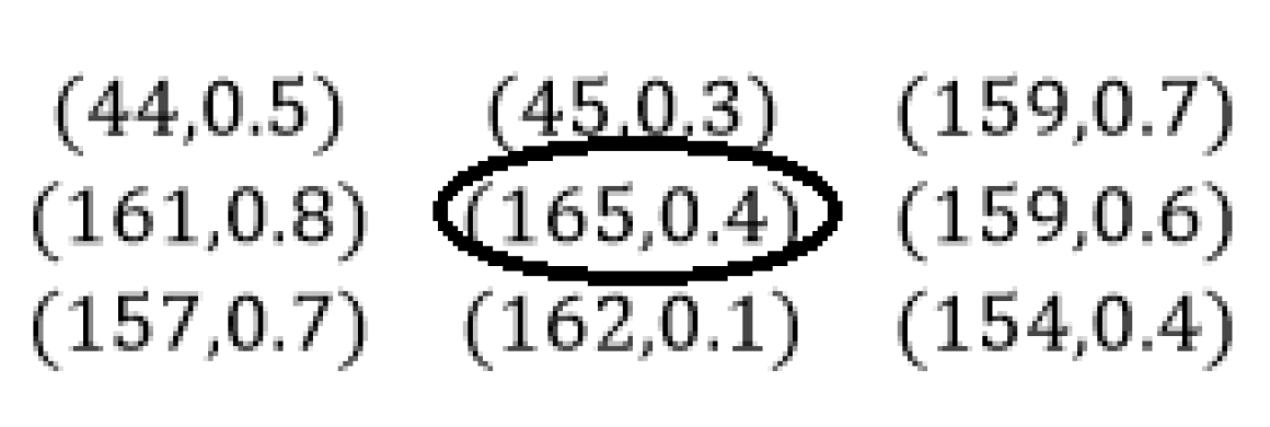
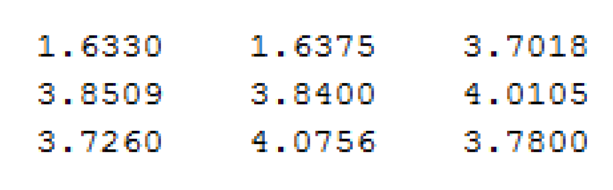
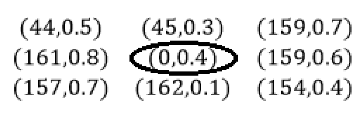
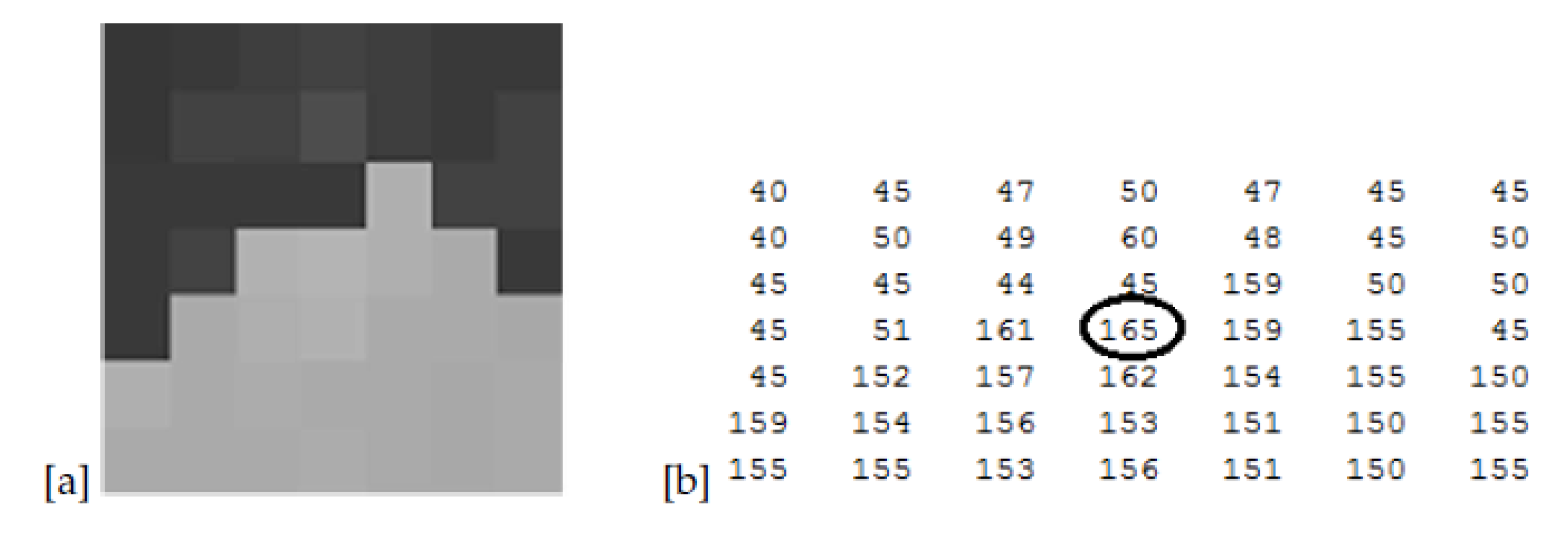
Example 3. Suppose the following matrix (Figure 1) is equal to the pixel values of a part of an image on a gray scale. For each pixel, the amount of gray is expressed as a symmetric triangular fuzzy number. We want to use to estimate the value of 165 in the above matrix. Now, using Equation (5), we calculated the value of each pixel in the neighborhood of 165 and considered the pixel that has the largest as the best alternative to the value of 165. Note that in Figure 2 the maximum value in matrix is , which corresponds to pixel number . Therefore, the value of this pixel, , can be chosen as the best alternative to the neighborhood matrix center. To express the accuracy of this method, we assumed that a noise is added to the image so that the neighborhood matrix is as follows (Figure 3): The maximum value in matrix (Figure 4) is , which corresponds to the pixel number . Therefore, the value of this pixel, , is the best estimate for the center of the neighborhood matrix. 6. Fuzzy Amount of Pixel’s Color
One of the important points in using the algorithm presented in the previous section is to assign or calculate a fuzzy number for the color of each pixel. Since the color value of each pixel is expressed as a crisp number, different approaches to their fuzzy expression can be suggested, which can provide a field of study for future research. For a better explanation of the subject, it should be noted that just as the colors of a rainbow cannot be easily separated and the colors are slowly converted, the difference between the color of a pixel and the color of its neighborsis difficult. Fuzzy sets can easily do this, while in existing algorithms, a non-negative integer is considered for the color of each pixel.
Our approach in this paper is to use the neighborhoods of a pixel to express the fuzzy color of the desired pixel. In other words, we assumed that the color of each pixel is an asymmetric triangular fuzzy number, the color of each pixel being determined by the degree of membership 1 and its left or right width by the mean of k means generated by the bootstrap resampling method where k is the number of sampling repetitions of the desired pixel neighborhoods. We used the bootstrap resampling method to reduce the effect of the outliers in the selected window. One of the main reasons for using the bootstrap is that this sampling is based on the sample we have. Often, this sample is the only source we have for research, and this adds to the importance of the bootstrap method. Since the bootstrap reliability improves with the number of bootstrap repetitions, we can obtain a more reliable estimate of the mean value of the central pixel neighborhoods by increasing the number of samples.
The bootstrap method provides an estimate of a quantity of a population. This is achieved by collecting small samples repeatedly, calculating the statistics, and averaging the calculated statistics. This procedure can be summarized in the following terms:
Select a number of bootstrap samples to perform;
Select a sample size;
For each bootstrap sample:
- a
Draw a sample with replacement with the chosen size;
- b
Calculate the statistic on the sample;
Calculate the mean of the calculated sample statistics.
For example, if the image is grayscale, we have only one color number for each pixel. Consider a window of its neighborhoods of each pixel (except in the pixels of the image margin), and calculate the mean of the bootstrap means.
The obtained number is a triangular fuzzy number with a right or left width. For example, suppose the pixel color is 50 and the mean of the bootstrap means is 60. Consider the color of a pixel as a fuzzy number
, with the left width of zero (because the mean of the bootstrap means is larger than the desired pixel) and the right width of 10 (which is equal to the difference between the pixel value and the mean of the bootstrap means). In the next example (Morillas et al. [
15]), we give a more detailed description of the algorithm.
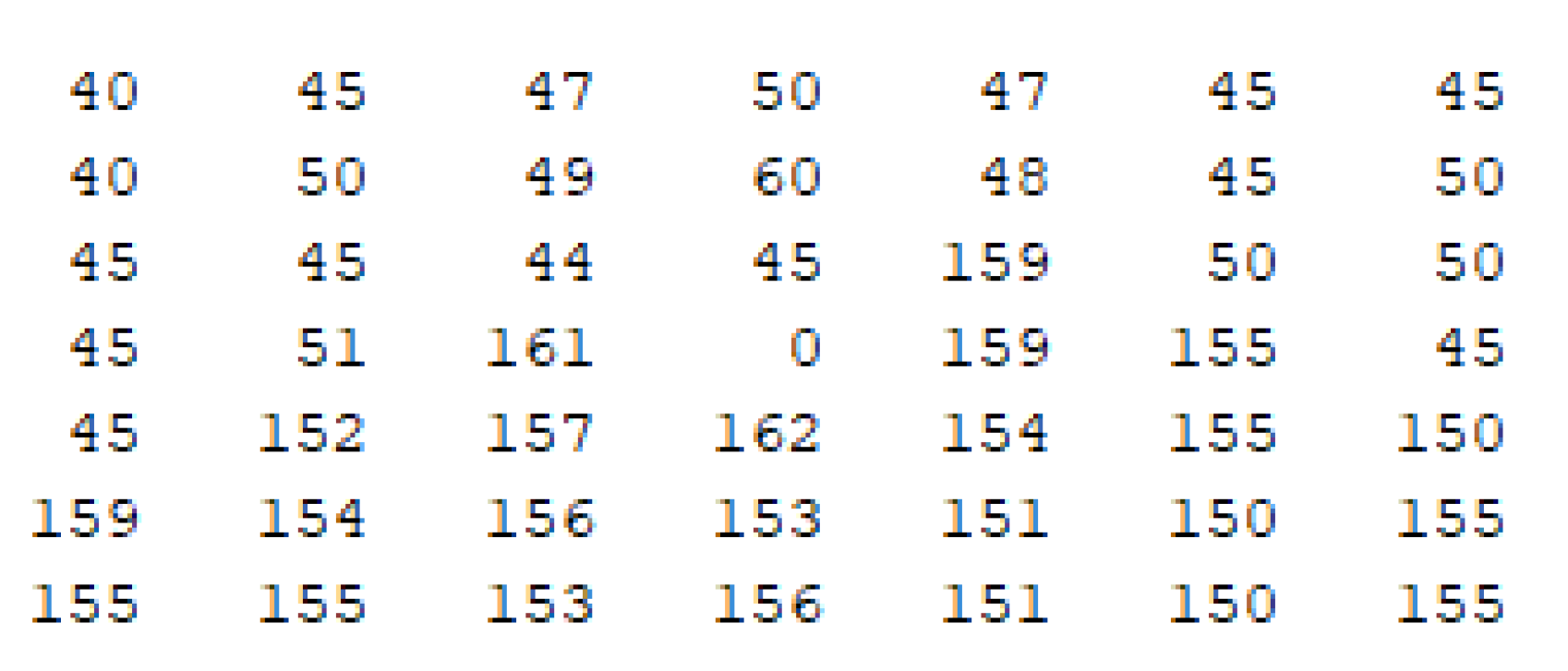
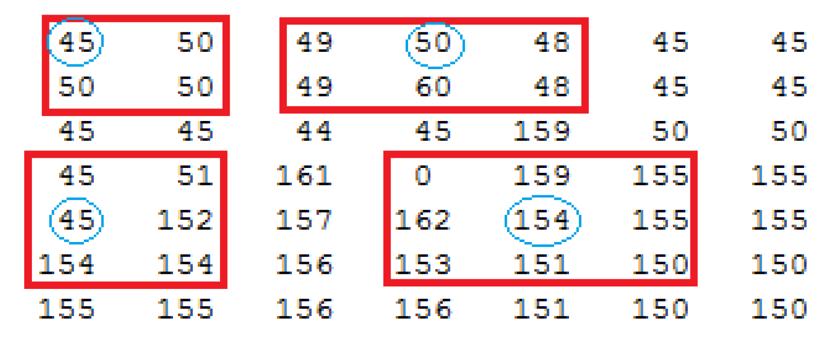
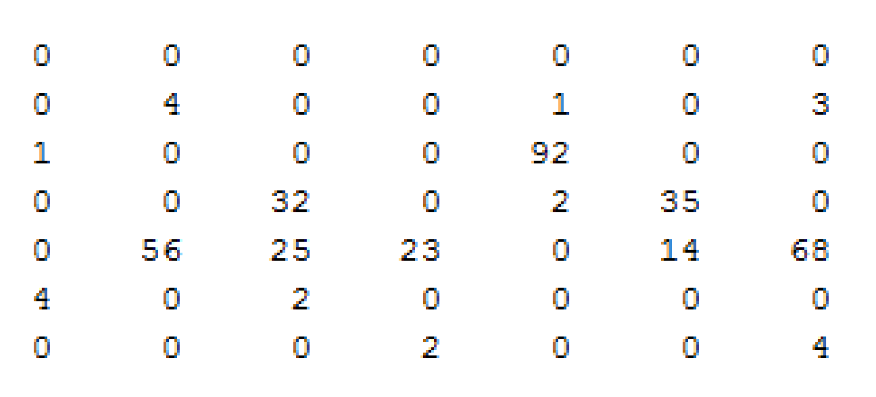
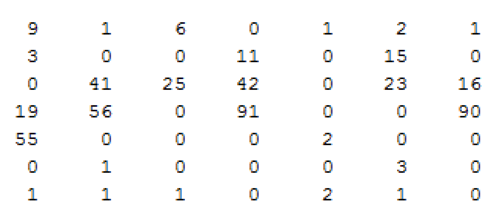
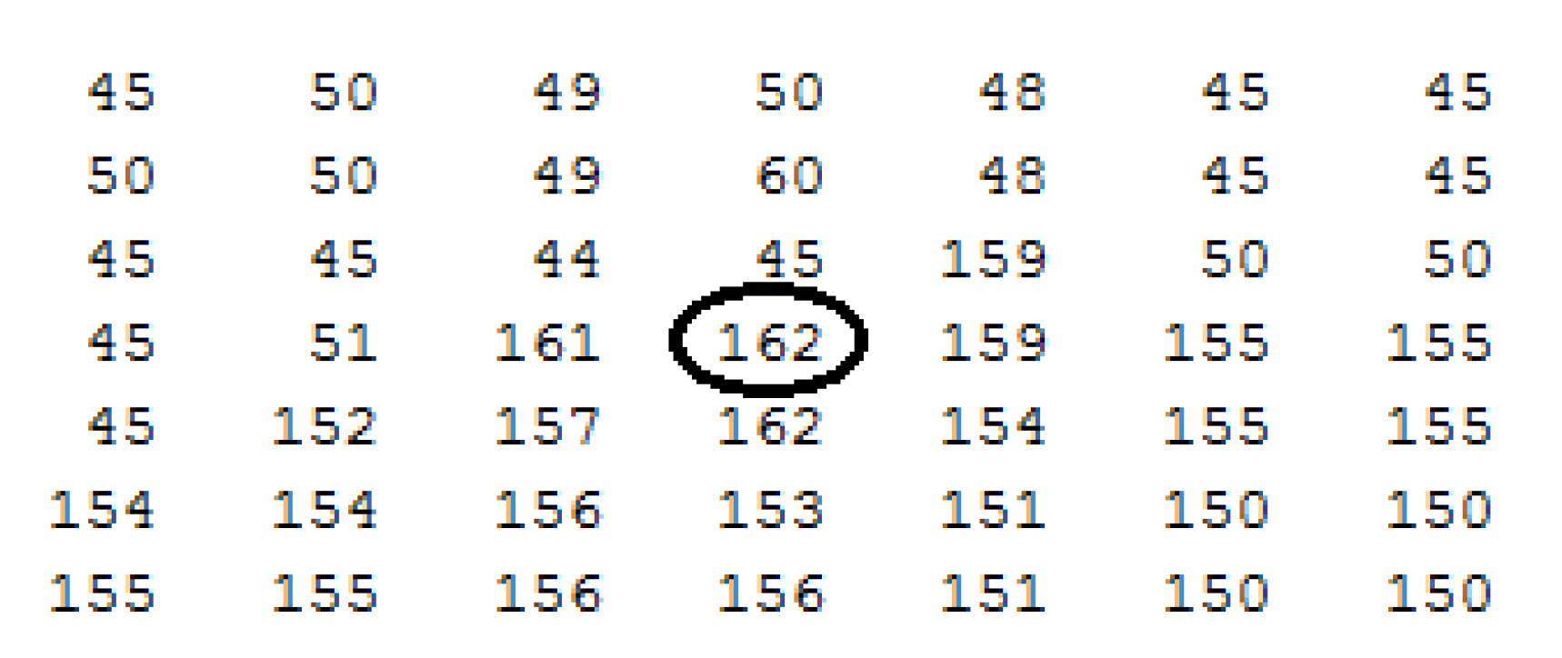
Example 4. Suppose the following matrix is equal to the values of the pixels in the image on a grayscale (Figure 5). Now, if there is noise in the image, we can eliminate the noise using the fuzzy approach. Suppose we replace the middle pixel of the image (165) with the value of 0, what is shown in Figure 6. To convert the color matrix of pixels, it is necessary to select each pixel and its nearest neighbors (a , or , or matrix for the side pixels and a matrix for the other pixels, similar to Figure 7). Then, using bootstrap sampling, we obtain the mean of the neighborhoods. Now, if the mean of the neighborhoods is smaller than the center pixel, the pixel becomes a triangular fuzzy number the left width of which is equal to the difference of the pixel with the mean and the right width of which is equal to 0, and if the mean is greater, it is the product of the fuzzy number with the right width. After calculating the left or right width of each pixel, the results can be seen in Figure 8 and Figure 9. The left width is as follows.
Figure 8.
Left width of the fuzzy matrix.
Figure 8.
Left width of the fuzzy matrix.
Figure 9.
Right width of the fuzzy matrix.
Figure 9.
Right width of the fuzzy matrix.
Now, we eliminated the noise by performing the algorithm described in this section. We know that and are two asymmetric triangular fuzzy numbers as follows: where is the left width and is the right width. Then, and will be equal to: Now, the estimate of the noisy pixel for 10 repetitions in bootstrap sampling is shown in Figure 10: It can be seen that the value of this pixel (162) is the best estimate for the center of the matrix, which was 165 as the actual value. That is, while using the median filter, the alternative value will be equal to 157. Of course, it should be noted that to achieve a convergence in estimation, it is necessary to increase the number of iterations.
In the following, as a real example, we removed the noise from the gray and color images. First, for the gray image, we examined the lung CT scan image related to the COVID-19 virus. Then, we used the images of Lenna and Baboon for the color images. For each image, we compared the result of the filter presented in this paper with the median filter and using the mean absolute error () and peak signal-to-noise ratio ().
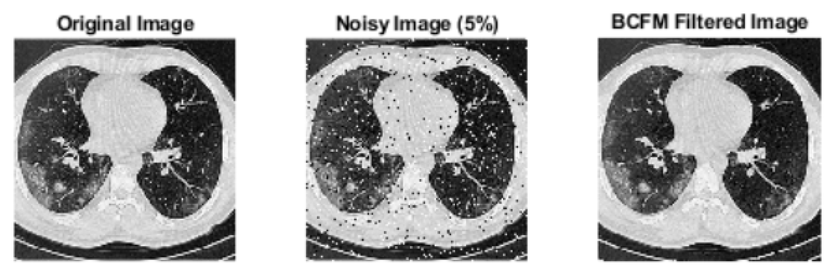
Example 5. A lung CT scan is a common imaging tool for diagnosing pneumonia. CT scans provide high-quality images of lung tissue, and the radiologist can quickly determine the extent of lung involvement with the disease. A CT scan of the lung reveals common radiological features in patients with COVID-19 pneumonia. Noise in medical images can make it difficult to diagnose COVID-19. In this section, we remove the noise from the lung CT scan image in a patient with the COVID-19 virus by using the filter. To show the power of the filter for fuzzy sets in noise removal or reduction, we first added noise (salt and pepper of 5 and 10 percent) to the initial image.
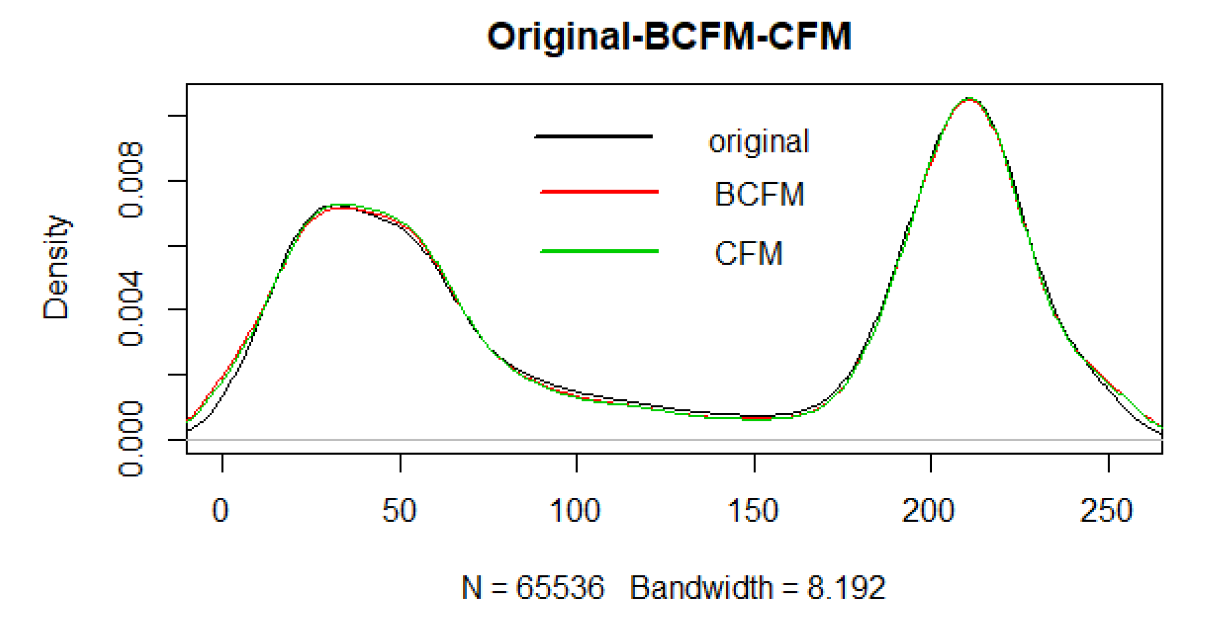
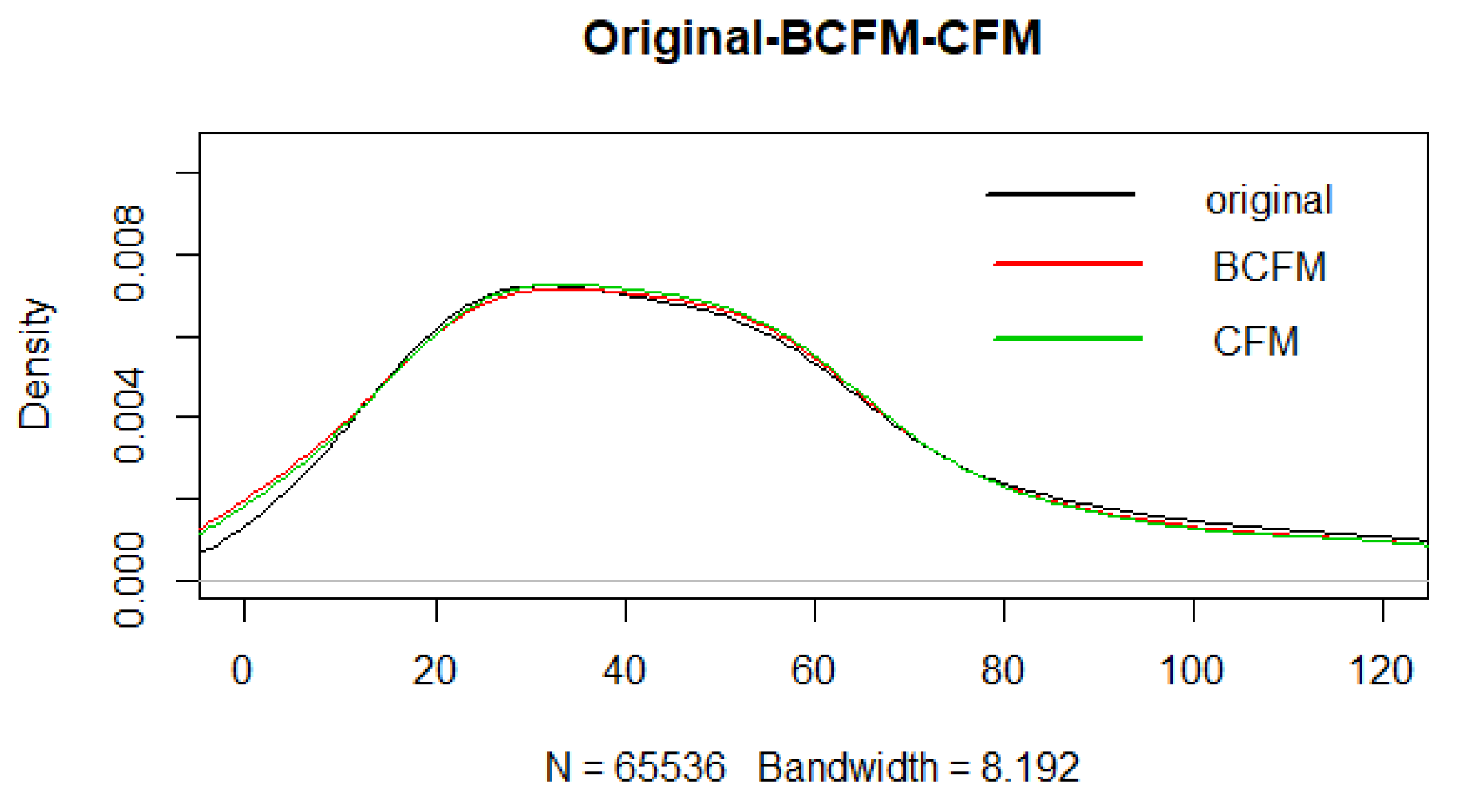
After using the filter, the results are in Figure 11 and Table 1. As we can see in Table 1, the filter has the lowest and the highest among the three filters , , and . Furthermore, as the number of bootstrap samples increases, and will converge to the minimum and maximum values, respectively. To better compare the two methods and , we can use the probability density graph of images. Figure 12 shows the density of the original image in black, in green, and in red. Whichever density of green or red is closer to the density of black indicates the better performance of the method. Careful examination of the densities shows that, except in the range of 0 to about 30, the red density is closer to black, and in general, it can be said that the red density performs better in most places or is similar to the green density. To better illustrate this point, we see a slice of the graph in Figure 13. By observing the image details and examining the pixels, it is observed that has a softer approach to image details than . In other words, the modified image loses more detail by the method, and this can be a reason for the better performance of .
Example 6. In this example, we compared the performance of the filter in color images with other methods. For the performance comparison, we used the and for different densities of noise for the test images.
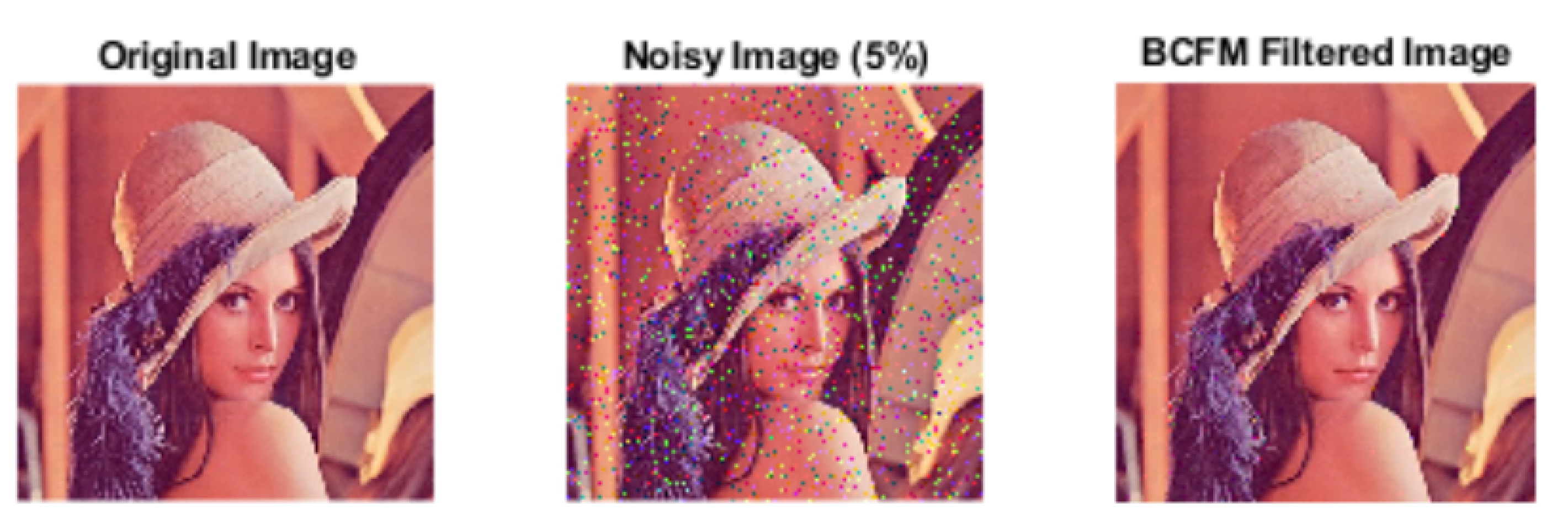
Here, we added 5 and 10 percent noise (salt and pepper) to the images of Lenna and Baboon. The results of the filter with the number of bootstrap samples being 10, 20, and 50 are reported in Figure 14 and Figure 15 and Table 2 and Table 3.
Figure 14.
1. Original Lenna image. 2. Noisy image after adding noise. 3. BCFM filtered image for bootstrap resampling.
Figure 14.
1. Original Lenna image. 2. Noisy image after adding noise. 3. BCFM filtered image for bootstrap resampling.
Table 2.
Comparison of the performance of the noise reduction filters for the Lenna image.
Table 2.
Comparison of the performance of the noise reduction filters for the Lenna image.
| Noise Percentage | Filter Evaluation | Median Filter | CFM Filter | BCFM Filter |
|---|
| | |
|---|
| 5 | MAE | 2.2008 | 0.3244 | 0.2871 | 0.2862 | 0.2851 |
| 5 | PSNR | 28.2372 | 32.2956 | 32.5741 | 32.6900 | 32.6968 |
| 10 | MAE | 2.3839 | 0.5766 | 0.5513 | 0.5500 | 0.5498 |
| 10 | PSNR | 27.2823 | 30.3462 | 30.5876 | 30.6003 | 30.6152 |
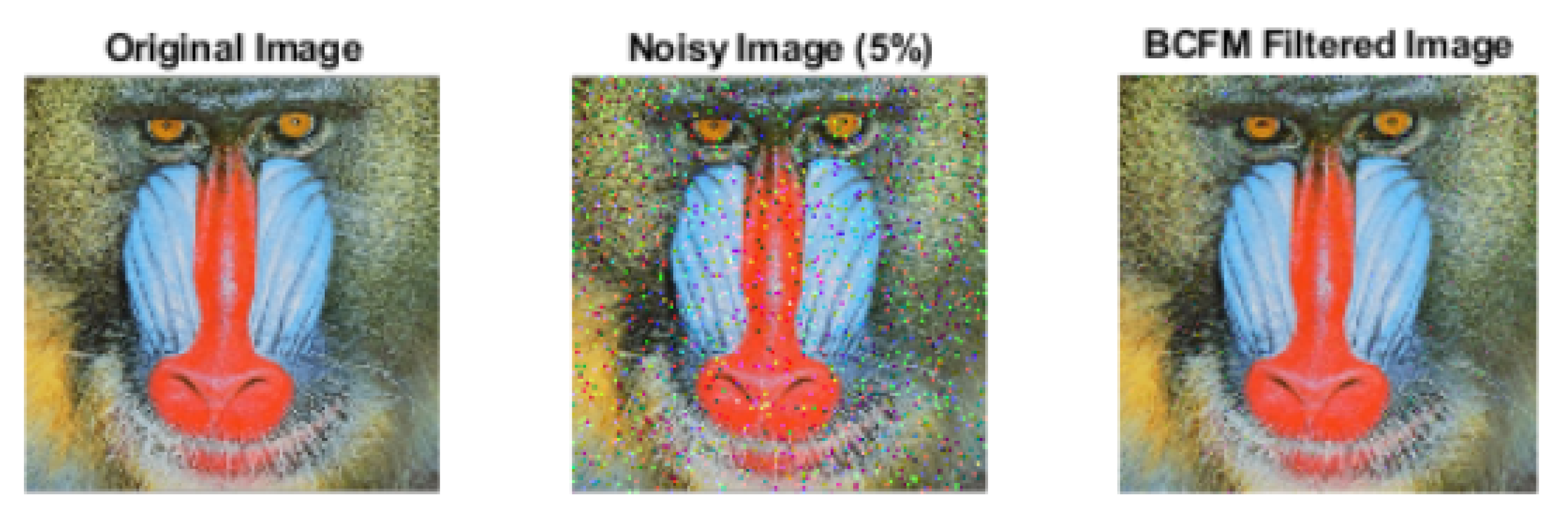
Also, for the image of Baboon, the results are as follows:
Figure 15.
1. Original Baboon image. 2. Noisy image after adding noise. 3. BCFM filtered image for bootstrap resampling.
Figure 15.
1. Original Baboon image. 2. Noisy image after adding noise. 3. BCFM filtered image for bootstrap resampling.
Table 3.
Comparison of the performance of the noise reduction filters for the Baboon image.
Table 3.
Comparison of the performance of the noise reduction filters for the Baboon image.
| Noise Percentage | Filter Evaluation | Median Filter | CFM Filter | BCFM Filter |
|---|
| | |
|---|
| 5 | MAE | 4.5121 | 1.1825 | 1.0452 | 1.0422 | 1.0406 |
| 5 | PSNR | 24.7003 | 27.9888 | 28.3880 | 28.3888 | 28.4157 |
| 10 | MAE | 4.6989 | 1.5336 | 1.3862 | 1.3841 | 1.3799 |
| 10 | PSNR | 24.3602 | 27.0842 | 27.4901 | 27.4877 | 27.4813 |
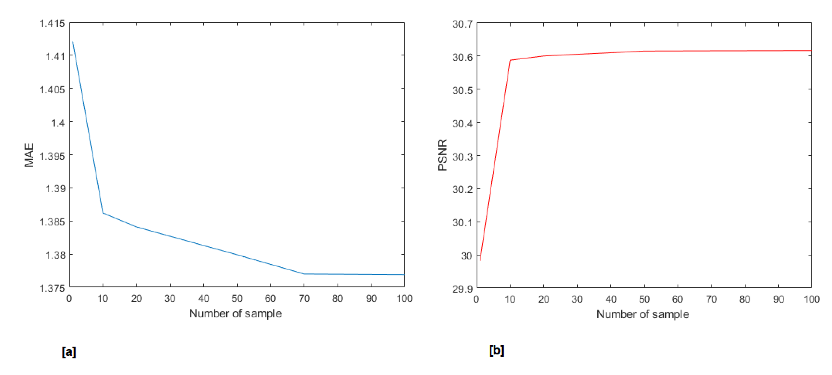
Figure 16 shows how and converge to the minimum and maximum values as the sample size increases, respectively. Clearly, Table 2 and Table 3 also confirm the results shown in Example 5 for color images. 7. Conclusions
Colors are one of the places where the fuzzy concept can be greatly used. If we express the color of each pixel as a fuzzy number in an image, we can separate the color of the pixels more accurately. In this paper, we introduced an approach to determine the fuzzy color value of each pixel and reduce the noise of an image by using convergence in the mean bootstrap (according to the
in the fuzzy metric space [
14]).
In fact, the
filter relies on the
for the bootstrap mean [
14], eliminates noise, and as shown in the results, performs better than the
and
filters.
Two reasons can be considered the main factors improving the results. The first reason can be seen in the use of the fuzzy color pixel approach, which, according to the expressed triangular fuzzy number for each pixel, finds a more accurate mean of the central pixel neighborhoods of each window. The second reason for the performance improvement can be expressed by using the bootstrap mean to calculate the mean of the neighbors, which, by increasing the sample, reduces the effect of outliers (noisy pixels) on the mean. In 2007, Morillas et al. [
15] compared the
filter to other methods, and the results showed that
performed better than the other filters. In this paper, we compared the
filter with
, which shows the better performance of the
filter compared to the other methods.


