Deep Reinforcement Learning for Vehicle Platooning at a Signalized Intersection in Mixed Traffic with Partial Detection

Abstract

The intersection management system can increase traffic capacity, vehicle safety, and the smoothness of all vehicle movement. Platoons of connected vehicles (CVs) use communication technologies to share information with each other and with infrastructures. In this paper, we proposed a deep reinforcement learning (DRL) model that applies to vehicle platooning at an isolated signalized intersection with partial detection. Moreover, we identified hyperparameters and tested the system with different numbers of vehicles (1, 2, and 3) in the platoon. To compare the effectiveness of the proposed model, we implemented two benchmark options, actuated traffic signal control (ATSC) and max pressure (MP). The experimental results demonstrated that the DRL model has many outstanding advantages compared to other models. Through the learning process, the average waiting time of vehicles in the DRL method was improved by 20% and 28% compared with the ATSC and MP options. The results also suggested that the DRL model is effective when the CV penetration rate is over 20%.

1. Introduction

Nowadays, traffic congestion is a major challenge, especially in large cities during rush hour [1]. It increases the delay time at intersections, increases fuel consumption, and reduces average speeds and discomfort when traveling [2]. Traffic congestion occurs when the travel demand exceeds the capacity of the available infrastructure. Many solutions can ease traffic congestion and balance the travel demand and road capacity. However, expanding the road network and increasing the number of lanes is very expensive and challenging in places where it is difficult to clear the ground, such as urban areas [3].

Much research has been conducted to upgrade transportation infrastructure and create new protocols using modern technologies to improve vehicle-to-vehicle (V2V) and vehicle-to-infrastructure (V2I) communication [4]. With the advancement of science and technology, cooperative intersection management (CIM) has helped automobile drivers significantly when traveling on the road [5]; for example, vehicles communicate with each other and with the infrastructure to select the optimal traffic management policy. Given the advantages of connected vehicles (CVs), they will become popular in the future with further advancements in science and technology [6].

In addition, emerging technologies in the automotive sector and wireless communication have increased the ability to improve vehicle maneuverability without expanding the existing road network [7]. CVs are a new solution to improve road capacity, reduce traffic congestion, and increase traffic speed in urban areas while retaining the current road network systems [8]. These new technologies facilitate drivers, improve traffic, and increase the level of service (LOS) at intersections.

According to [9], CVs share V2V information directly with each other via wireless communication. This paper also indicated that the distance between CVs was smaller than that between regular vehicles (RVs). This was explained by the fact that CVs can promptly perceive information about surrounding vehicles (position, speed, acceleration), as well as V2I communication through the use of dedicated short-range communications (DSRC). Other papers also showed that using CVs brings significant benefits related to traffic measures of effectiveness (MOEs), passenger comfort, and pollution reduction.

In recent years, many studies have also analyzed the effects of CVs on the road and proposed new car models based on existing models [10,11]. These papers attempted to describe the behavior of CVs, such as conventional vehicles, but only under certain specific conditions, without providing a full generalization model. Another paper concluded that CVs provide a significant road safety benefit by increasing the proportion of CVs in the model [12]. It has been estimated that the rate of traffic conflicts can be reduced by up to 90% when the percentage of CVs is 100%.

The introduction of vehicles equipped with adaptive cruise control (ACC) or cooperative adaptive cruise control (CACC) can considerably enhance driver assistance and improve the road’s capacity. Many papers have focused on assessing the influence of vehicles equipped with CACC on reducing congestion and improving traffic efficiency. Liu et al. [13] simulated and evaluated the impact of CACC market penetration on the capacity of the multilane freeway merge bottleneck. This system mainly controlled the longitudinal movement between the preceding vehicles based on the distance between the two vehicles and the difference in speed. Many algorithms related to CACC have been proposed to control vehicles in terms of safety and increase traffic efficiency. Zohdy et al. [14] proposed an optimization tool to optimize the movements of vehicles equipped with CACC instead of the traditional management method. Arem et al. [15] introduced a model for CACC-equipped vehicles that is based on the relative speed, safe deceleration, current acceleration, and the distance between vehicles, to determine the desired acceleration at the next step. By using the microscopic model for simulation of intelligent cruise control (MIXIC) simulation model, the paper focused on the effects of CACC on traffic flow. Its results showed that it is possible to establish a stable and sustainable traffic flow and increase traffic efficiency compared to the traditional scenarios.

Much research has also been conducted to group CVs into platoons to enhance vehicle performance. Segata [16] defined a platoon as an application to improve the mobility of vehicles by utilizing DSRC to share information, reducing the distance between vehicles when forming a group. The author also developed PLEXE, a tool combined with the Veins vehicular networking framework, to simulate the platoon system accurately. A simulation model was created with PLEXE to run experiments in scenarios with V2V communication [17]. Two types of experiments were performed to demonstrate the efficiency of the model: controller analysis and join maneuver. However, these models only consider platoons moving in a straight line, not considering the influence at the intersection area or the communication between vehicles and infrastructure. The authors in [18] provided an overview that categorized influencing factors for platoons. The structure of platoon vehicles remains an open and challenging topic. However, the model only includes the desired destination and arrival time as input data used for calculation. Other aspects are omitted due to complexity reasons. In [19], the authors proposed an intra-city transportation service based on connected autonomous platoon systems. The paper aimed to analyze the influence of the platoon system on travel time and develop an algorithm for the behavior of platoons at the roundabout. However, the authors only considered travel time. Other traffic factors of the system have not been fully presented.

RVs significantly impacted the platoon formation in mixed traffic compared to the ideal case [20]. Another result of this paper was that platoon formations might not maintain their desired speed, leading to temporary traffic delays. The position of CVs determined car-following models and the formation of the platoon. Simulating a platoon was completely different from simulating a free flow as the platooning vehicles needed to maintain a constant distance between them [21]. This distance can be changed in the case of free-flow vehicles. This paper has proposed a model to analyze the platoon’s behavior in the mixed traffic flow. However, this study only focused on analyzing the platoon merging operation. Other papers [22,23] also developed platoon organization strategies based on local traffic states. CVs could form longer platoons but cause more lane changes in mixed flow. These lane changes did not significantly impact traffic performance at low traffic levels. However, many lane changes could reduce capacity and cause traffic congestion at high traffic levels. Therefore, it was reasonable to propose a platoon organization strategy to enhance platoon formation without reducing traffic performance [24].

Platoons possessed great potential to improve roadway capacity, but there were a number of factors that affected the platoon configuration, such as the inter-platoon gap, intra-platoon gap, platoon size, and wireless communication, as shown in [25]. Platoon size (e.g., number of vehicles in a platoon) is a critical factor affecting model efficiency. Large-sized platoons improved model performance but reduced lateral maneuverability (e.g., lane change or merging) [26]. It was also shown that a high penetration rate improves traffic capacity and stability. Moreover, when the platoon size increased, the mean velocity decreased, and the velocity standard deviation increased, reducing the model’s stability. Other papers also expressed that overly large platoons affect traffic stability, making it difficult to manage platoons (merging and splitting) [27]. The research results also emphasize that the platoon size does not need to be too large, as this value is a trade-off between capacity and traffic stability.

In addition to the management of vehicle connections, intersection management policies also greatly affect traffic results. In the last decade, many major cities have changed their intersection management technologies to achieve better traffic efficiency. Instead of using traditional management methods (e.g., fixed time or stop signs), they have applied modern techniques, including adaptive traffic signals or intelligent traffic lights, combining cameras to determine traffic parameters to provide optimal scenarios. An actuated traffic signal controller (ATSC) used its algorithm, sensors, and Boolean logic to create a dynamic signal cycle. When traffic conditions changed, the ATSC automatically adjusted the active phase duration and cycle. The performance of signal light control depended on the optimization technique applied. Over the decades, there has been a great deal of research on signal light controllers based on techniques such as evolutionary algorithms [28,29], max pressure (MP) [30,31], self-organization [32], the Sydney coordinated adaptive traffic system (SCATS) [33], the split cycle offset optimization technique (SCOOT) [34] and adaptive control software lite (ASC-Lite) [35]. However, most of the algorithms used in signal light controllers consider the same aspects for all modes. Each mode in the traffic volume was treated equally. In addition, these algorithms also did not take full advantage of modern traffic data sources. Therefore, they were difficult to apply to intersections with high complexity.

Along with the development of science and technology, the input data of the deep reinforcement learning (DRL) model was also increasing. Deep neural networks (DNN) have been used to solve this complex problem to enhance model efficiency. Besides the traditional traffic management at intersections, reinforcement learning (RL) has also been used to manage adaptive traffic signal lights. In the past, due to technical limitations, models often had a small-sized state and used linear functions to approximate Q values. However, the complexity of the model was not fully demonstrated because of the limited input information. With the development of algorithms, DNN has been used to solve traffic problems such as autonomous vehicle training, signal optimization, traffic prediction, smart routing, etc. DNN was used to optimize signal lights and minimize waiting time [36,37,38]. In these models, the operation of traffic lights based on the traffic situation was defined in terms of actions, states, and rewards.

Researchers used DRL with proximal policy optimization (PPO) in a different approach to train autonomous vehicles and improve traffic performance [39,40]. Taking advantage of communication and CAV technology, Bai et al. [41] proposed a hybrid reinforcement learning (HRL) framework to control traffic at signalized intersections. To improve the driver’s behavior and optimize the signal lights, Zhou et al. [42] developed a deep deterministic policy gradient (DDPG) algorithm-based car-following model for CAVs. The results after the training process included optimizing the traffic signals and adjusting the vehicle’s trajectory behavior to ensure the minimum waiting time. In addition, some authors have also optimized signal lights with platooning vehicles in some papers [43,44,45]. Research results show that combining reinforcement learning with information sharing (V2V and V2I) improved the traffic model very effectively. The results after training depend on the set of random seeds and other parameters. The intersection management performance of the DRL-based approach was higher, but the input data requirements were more complex.

In general, most popular models often assumed that all vehicles were detected to collect information. This was not true because only vehicles equipped with a wireless communication system could be connected. Nowadays, many new technologies are used to better connect the information between the vehicle and the intersection management system (IMS). Traditional devices such as loop detectors can only detect the presence of vehicles when passing them. However, new devices (such as DSRC, GPS localization, and Bluetooth) are cost-effective and can collect more data (speed, distance from CVs) continuously. The increased number of connected vehicles increases the ability to transmit information between vehicles with the IMS [46,47]. However, these papers did not study platoon formation between CVs. By merging CVs into platoons, it will greatly improve road capacity and other parameters.

It can be seen that the combination of platooning vehicles and DRL is an excellent solution to improve the existing traffic problem. To achieve this purpose, we proposed the DRL method with platooned vehicles at a signalized intersection with partial detection. To compare the effectiveness of the proposed model, we implemented two benchmark options, ATSC and MP. These scenarios were all simulated with the change in platoon size (from 1 car to 3 cars in a platoon). The main contributions of this study are as follows.

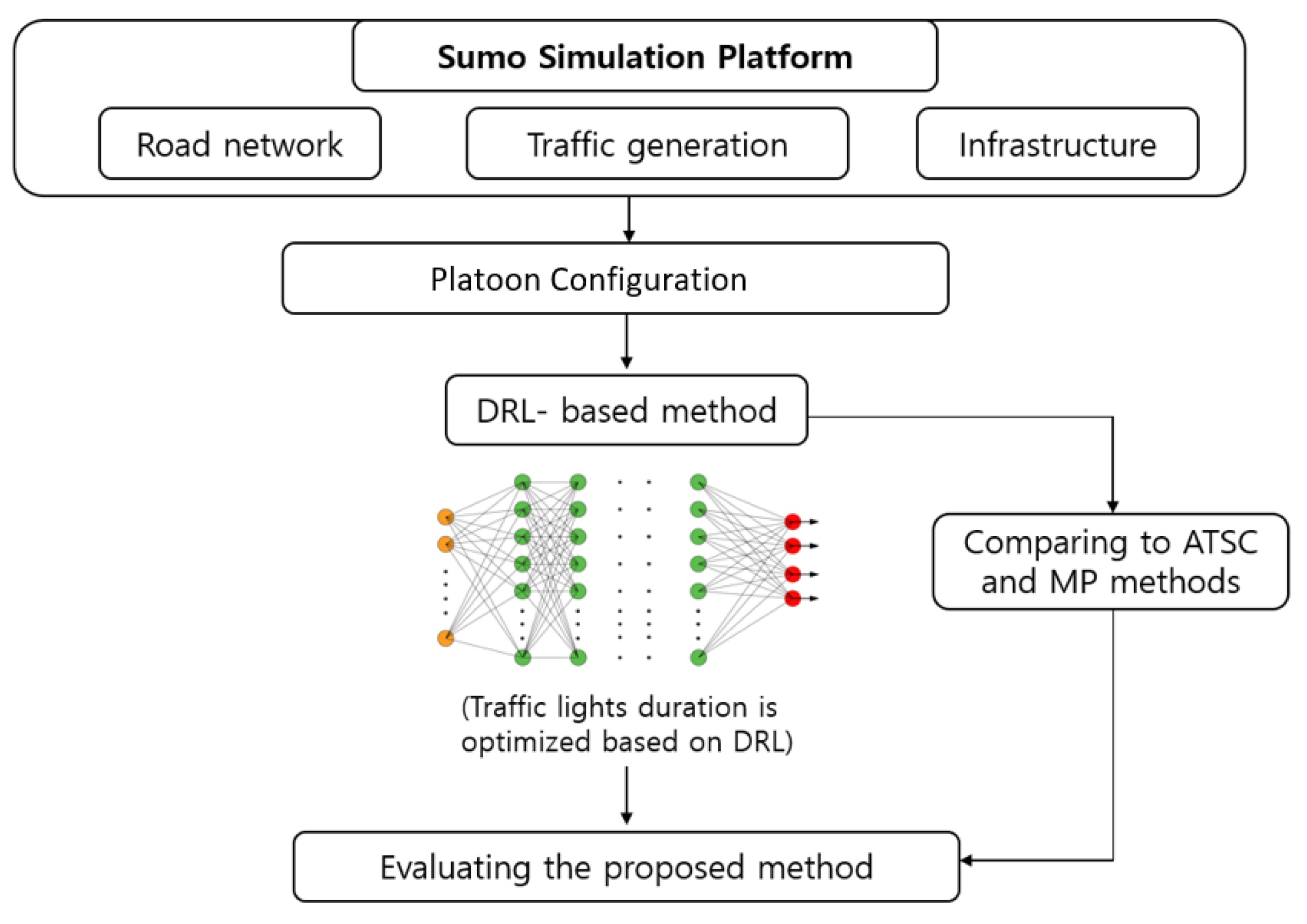
• We combined systems that work together, including platoon and DRL, with partial detection at a signalized intersection. DRL was the main solution to improve signal system optimization and traffic efficiency. We proposed a new state description for the mixed traffic (IMS only collected information from platoon vehicles (CVs)). Compared with two benchmark options, ATSC and MP, the proposed solution reduced the waiting time of all vehicles significantly.
• A set of hyperparameters was tested to identify the main influencing parameters in the learning process.
• We also considered the effect of platoon size (number of vehicles in the platoon) at the intersection to measure the average delay time, waiting time, speed of traffic, and travel time. The contribution of this paper increased the understanding of the influence of platoons at signal intersections.
• Finally, we evaluated the influence of CV penetration rate on the model results and recommended reasonable rates.

The rest of the paper follows: Section 2 presents the research methodology. Section 3 presents the experimental setup. Section 4 contains the results of traffic simulations and evaluations. Section 5 and Section 6 give the discussion and conclusions.

2. Research Methodology

2.1. Research Architecture

We simulated an isolated signalized intersection by SUMO (Simulation of Urban Mobility tool) [48] with different platoon sizes and traffic scenarios. The proposed DRL model was implemented by Python programming and the Tensorflow module. Platooning in the model was simulated by the Simpla plugin [49], which can define the specific behavior of platooning vehicles. Simpla creates new additional vehicle types that describe platooning modes. SUMO TraCI (traffic control interface) protocol [50] uses TCP-based client/server architecture to provide access to Sumo and retrieve values from the simulation model.

The performance of these models is measured on an Intel Core i9-10,900 computer with 64 GB ram. This work integrates platooning vehicles and DRL at a signalized intersection to enhance the quality of traffic flow. Firstly, we used the SUMO simulation platform to generate a road network, traffic flow, and infrastructure. Secondly, the platooning vehicles were configured. Next, the DRL-based method was applied to optimize traffic lights. Finally, we implemented two benchmark options (ATSC and MP) and compared them with the proposed method. Three intersection management scenarios were tested to evaluate traffic measures of effectiveness (MOEs). The research architecture is shown in Figure 1 below.

2.2. Longitudinal Car-Following Models

The car-following model is a model used to describe the longitudinal interaction between vehicles in the same lane. Many car-following models are used in SUMO to mimic the behavior of conventional vehicles. The Krauss model is the most popular model used in Sumo and is also used in our traffic simulation. This safe-distance-based model assumes that the vehicle maintains a safe distance from the preceding vehicle and chooses its speed to ensure that it can stop safely to avoid collision [51]. This model could be expressed as follows:

$${\mathrm{v}}_{\mathrm{s}\mathrm{a}\mathrm{f}\mathrm{e}} (\mathrm{t}) = {\mathrm{v}}_{\mathrm{i}} (\mathrm{t}) + \frac{\mathrm{g} (\mathrm{t})-{\mathrm{g}}_{\mathrm{d}\mathrm{e}\mathrm{s}} (\mathrm{t})}{{\mathsf{\tau }}_{\mathrm{b}} + \mathsf{\tau }}$$

(1)

$${\mathrm{v}}_{\mathrm{d}\mathrm{e}\mathrm{s}} (\mathrm{t})= \min [ {\mathrm{v}}_{\max } , {\mathrm{v}}_{\mathrm{i}} (\mathrm{t}) +{\mathrm{a}}_{\mathrm{i}} (\mathrm{t}) {\mathsf{\Delta }}_{\mathrm{t}} , {\mathrm{v}}_{\mathrm{s}\mathrm{a}\mathrm{f}\mathrm{e}} (\mathrm{t})]$$

(2)

$$\mathrm{v} ( \mathrm{t}+ {\mathsf{\Delta }}_{\mathrm{t}} )= \max [ 0, {\mathrm{v}}_{\mathrm{d}\mathrm{e}\mathrm{s}} (\mathrm{t}) - \mathsf{\eta } ]$$

(3)

$$\mathrm{x} ( \mathrm{t}+ {\mathsf{\Delta }}_{\mathrm{t}} )= {\mathrm{x}}_{\mathrm{i}} (\mathrm{t}) +{\mathrm{v}}_{\mathrm{i}} {\mathsf{\Delta }}_{\mathrm{t}}$$

(4)

where x_i (t), v_i (t), a_i (t) are the position, speed, and acceleration of the vehicle at time t. ${\mathrm{v}}_{\max }$(t) and ${\mathrm{v}}_{\mathrm{d}\mathrm{e}\mathrm{s}}$ (t) are the maximum and desired speed of the vehicle. g (t) and ${\mathrm{g}}_{\mathrm{d}\mathrm{e}\mathrm{s}}$(t) are the gap distance and desired gap between vehicles at time t. τ is the driver reaction time, and η > 0 is a random perturbation to deviate from optimal driving.

2.3. Car-Following Models with Platoons

There are many tools that utilize Sumo to create platoons, such as Simpla, Veins, and Plexe. Veins and Plexe combine wireless networking and a realistic vehicle environment based on the Sumo traffic simulator to implement platooning. However, the connection between them and Sumo is complicated because they require additional software for simulation. Simpla is a configurable platooning plugin for the TraCI Python client to create basic platooning logic and provide additional parameters.

To simulate our traffic model, we used Simpla and adjusted the current parameters to match the simulation conditions. Features of the platoon configuration in our model are as follows:

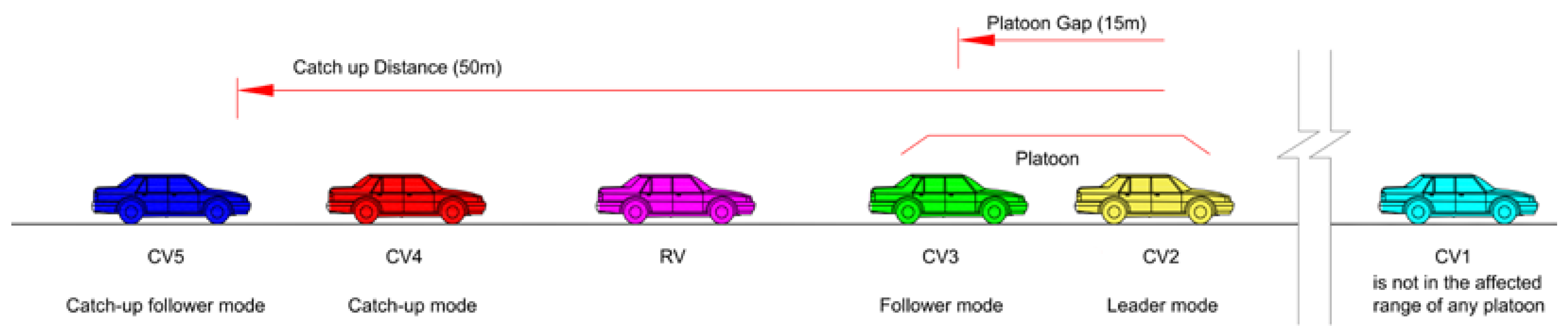
• When CVs are within the defined platoon range on the same lane, they can switch to 4 modes (platoon leader, platoon follower, catch-up, and catch-up follower mode), as shown in Figure 2. Platooning vehicles are considered as a platoon if the gap is smaller than 15 m (yellow and green vehicles). CVs switch their type to catch-up mode when the front platoon is closer to a given value of 50 m (red and blue vehicles). If the connection conditions are not met, CVs’ movement is similar to that of RVs (cyan vehicle).
• Changing lanes to join the platoon is not yet supported in Simpla. If the platoon leader changes lanes, other vehicles will try to change lanes.
• In the combined operation mode, when joining the platoon, CVs in the follower and catch-up modes can move at a speed greater than the maximum speed (speed_Factor equals 1.2). Other modes default to 1.
• A platoon leader has the ability to accelerate and switch to the follower mode if it is within range of another platoon in front.
• A platooning vehicle can switch to the manual mode if it is outside of the platooning range. It can accelerate and connect to form a platoon in a catch-up area.
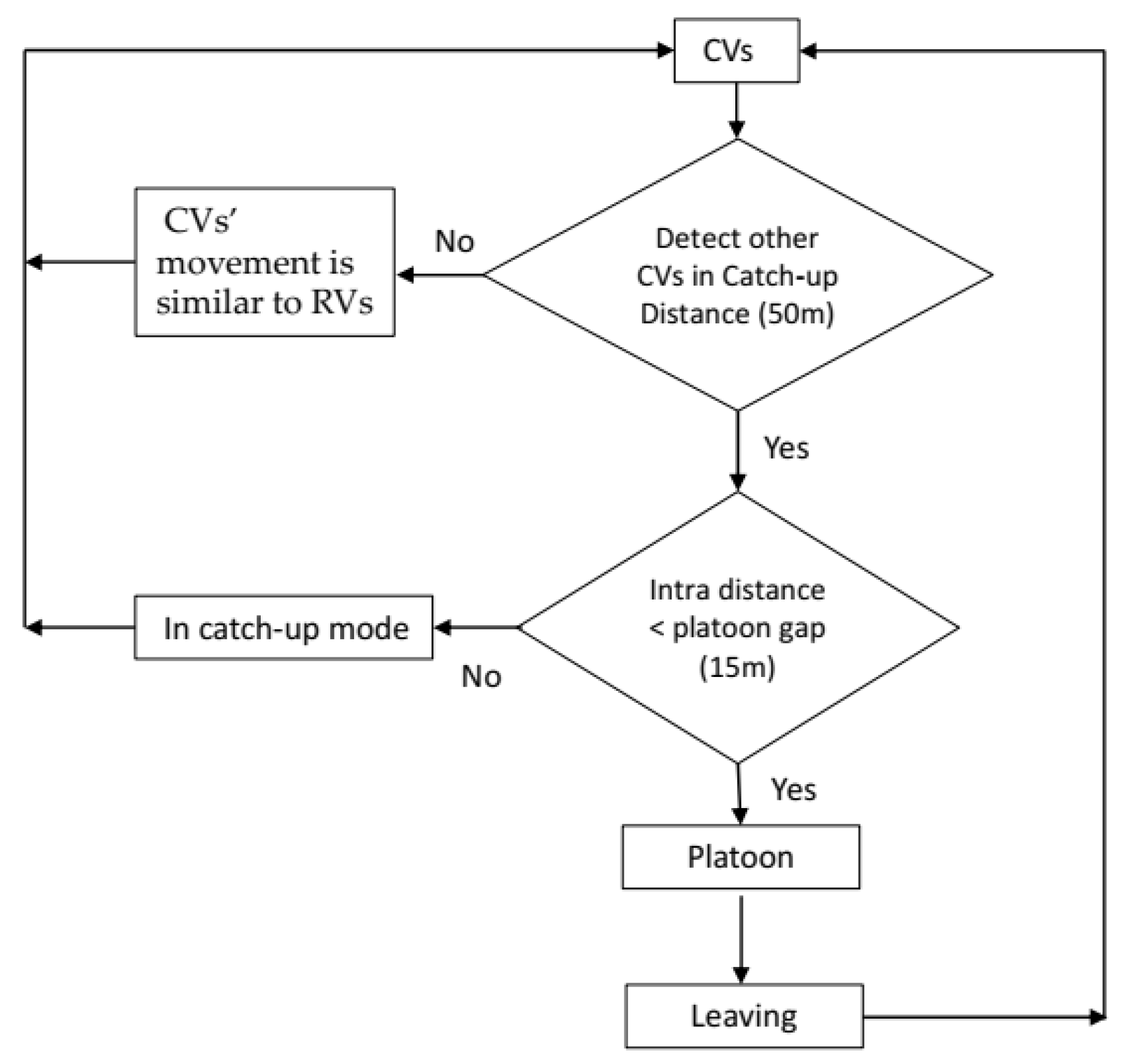
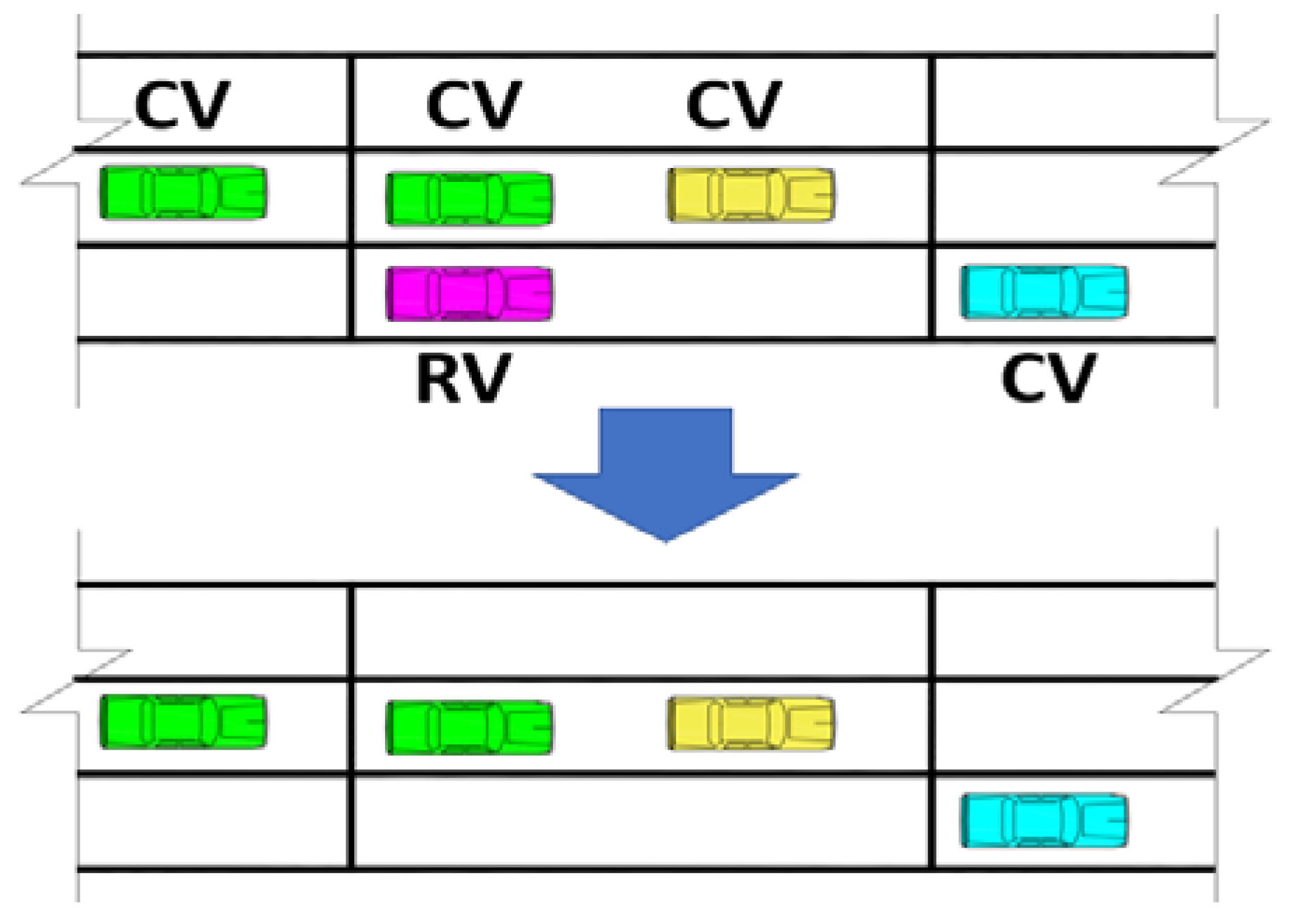
• At the intersection area, due to the influence of traffic lights, CVs can be split from the platoon. The reforming of the platooning operation is shown in Figure 3.

We assumed that the platoon configuration was perfect, meaning that there was no damage, data package loss, or time delay during platooning operations. Vehicles in platoons try to maintain a safe distance from their preceding vehicles. Simulation experiments were performed with platoons of different sizes (the number of vehicles in the platoons varied from 1 to 2 and 3 vehicles). A safe distance between vehicles was an important factor in controlling the movement and characteristics of platoons [25]. To reduce the intra-platoon gap, we used a tau factor (minimum time headway) of 0.3 s for CVs. Our designed platoon protocol is presented in

Table 1. Attributes of platoons.

Parameter	Value
Platoon size	1, 2, and 3 vehicles
Vehicle length	4 m
Initial speed	5 m/s
Max_speed	20 m/s
Max_acceleration	2.5 m/s2
Max_deceleration	3 m/s2
Platoon gap	15 m
Catch_up distance	50 m
Speed_factor	1.2 only for follower and catch-up modes. 1 for other modes
tau (The desired minimum time headway)	0.3 s for CVs and 1 s for RVs.
minGap	0.5 m for CVs and 2.5 m for RVs

below.

The movement of the leader vehicle in platoons is affected by the inter-platoon gap. If the distance is smaller than the safe distance, the platoon will decelerate according to the car-following model until this distance increases to a safe distance. The following vehicles in the platoon adjust their acceleration and speed according to the leader. Thus, the platoon’s formation is dynamic when it moves through the intersection.

2.4. Learning with DRL

RL is based on algorithms for learning through experiences between agents and the environment without prior information. In RL, agents employed in an unknown environment interact with their environment and take appropriate actions to maximize their performance. Based on selected actions, the scalar reward (positive and negative) is obtained, and the agent continues to learn until it reaches the highest performance. The RL model can be expressed by a four-tuple (S, A, R, T), in which S, A, R, and T are the possible state space, action space, reward space, and the transition function of the model.

At each time t, the agent selects an action ${\mathrm{a}}_{\mathrm{t}}$, takes a reward ${\mathrm{r}}_{\mathrm{t}}$, and moves from a state ${\mathrm{s}}_{\mathrm{t}}$ to a new state ${\mathrm{s}}_{\mathrm{t}+1}$. The core of the algorithm is a Bellman equation, using the weighted average of the old and the new information value.

$${\mathrm{Q}}^{\mathrm{n}\mathrm{e}\mathrm{w}} ({\mathrm{s}}_{\mathrm{t}}, {\mathrm{a}}_{\mathrm{t}}) = {\mathrm{Q}}^{\mathrm{o}\mathrm{l}\mathrm{d}} ({\mathrm{s}}_{\mathrm{t}}, {\mathrm{a}}_{\mathrm{t}}) + \mathsf{\alpha } ( {\mathrm{r}}_{\mathrm{t}}+\gamma \mathrm{Q}{ }^{\max }( {\mathrm{s}}_{\mathrm{t}+1}, {\mathrm{a}}_{\mathrm{a}})-{\mathrm{Q}}^{\mathrm{o}\mathrm{l}\mathrm{d}} ({\mathrm{s}}_{\mathrm{t}}, {\mathrm{a}}_{\mathrm{t}}) )$$

(5)

Here,

• ${\mathrm{Q}}^{\mathrm{n}\mathrm{e}\mathrm{w}} ({\mathrm{s}}_{\mathrm{t}}, {\mathrm{a}}_{\mathrm{t}}), {\mathrm{Q}}^{\mathrm{o}\mathrm{l}\mathrm{d}} ({\mathrm{s}}_{\mathrm{t}}, {\mathrm{a}}_{\mathrm{t}}), {\mathrm{Q}}^{\max } ({\mathrm{s}}_{\mathrm{t}}, {\mathrm{a}}_{\mathrm{t}})$ are the updated, old and optimum Q network value.
• $\mathsf{\alpha }, \gamma$ are the learning rate and discount factor of the training network.

In this paper, we used the DRL-based approach to optimize traffic signals. Based on the data collected from the network system, the trained agent minimizes the waiting time of all vehicles to optimize the signal lights. The agent receives the current state of the network, the action of traffic lights, and the reward of the recent action while training. These data (${\mathrm{s}}_{\mathrm{t}}$, ${\mathrm{a}}_{\mathrm{t}}$, c${\mathrm{r}}_{\mathrm{t},\mathrm{t}+1}$) are stored in the experience replay and used while training.

The actions are selected based on different policies, where the agent can choose an action that does not have the highest Q value if it wishes to explore the environment. Alternatively, it can choose to exploit and choose an action with the highest Q value. The algorithm is expressed in Algorithm 1.

Algorithm 1: Training of deep Q network with Experience Replay on a traffic light.

Input: neural network agent with random weights, replay memory size, minibatch size, epsilon ($\epsilon$), learning rate ($\alpha$), and discount factor ($\gamma$)

Initialize replay buffer B in Memory M

Initialize action-value function Q with ${\theta }_o$

Initialize the action-value function $Q_n$ with random parameters ${\theta }_n = {\theta }_o$

while episode < Total Episodes:

Episode = 1, … E do

Start Simulation with first step J, observe initials state $s_o$ and action $a_o$

For J = 1, … N do

$Action = \{\begin{array}{c}Arbitrary with probability \epsilon \\ {\arg \max }_a^{\prime }Q (s_o, a_o, {\theta }_o), 1-\epsilon \end{array}$

Perform action $a_n$ and observe the reward r, next state $s_n$

Store experiences ($s_o, a_o, r, s_n$) in B.

Sample random B experiences from M

Calculate the loss L

$\mathrm{L} = \{\begin{array}{c}0,\hspace{1em}\hspace{1em}\hspace{1em}\hspace{1em}\hspace{1em}\hspace{1em}\mathrm{i}\mathrm{f}\hspace{1em}\mathrm{t}\mathrm{e}\mathrm{r}\min \mathrm{a}\mathrm{t}\mathrm{e}\mathrm{d}\\ \mathrm{r} + {{\max }_{\mathrm{a}}}^{\prime }{\mathrm{Q}}_{\mathrm{n}} ({\mathrm{s}}_{\mathrm{n}}, {\mathrm{a}}_{\mathrm{n}}, {\mathsf{\theta }}_{\mathrm{n}}), \mathrm{o}\mathrm{t}\mathrm{h}\mathrm{e}\mathrm{r}\mathrm{w}\mathrm{i}\mathrm{s}\mathrm{e}\end{array}$

Update ${\theta }_o$ by minimizing the loss function

${(L - Q (s_o, a_o, {\theta }_o))}^2 w.r.t \theta ;$

For every step

Reset $Q_n = Q_o$           Set $s_o = s_n$        end for

end while

3. Experimental Setup

3.1. Road, Lane and Other Configuration

The road network and traffic signals used for simulation were as shown in Figure 4 and Figure 5 with time steps of 0.1 s, a lane width of 3.5 m, and three lanes in each direction (one shared lane for going straight and turning right, one straight lane, and one left-turn lane), and the length in each direction was 500 m. The traffic flow was mixed flow, including platooning vehicles (yellow vehicles are leaders and green vehicles are followers) and RVs (magenta vehicles). In the figures, there are also red vehicles in catch-up mode, blue vehicles in catch-up follower mode, and cyan vehicles that are CVs but moving similarly to RVs because they are not within any platoon range. The model only collects data on platooning vehicles during training. Data on RVs are not collected. Based on the data collected, the model selects phases to optimize the waiting time for both CVs and RVs.

We gave several simulation scenarios to evaluate different aspects of the model. By varying the platoon size, we can model the traffic flow at sparse or dense levels. As mentioned in the introduction, the platoon size affected the model stability, and it is a trade-off between capacity and stability. Because urban intersections entail many constraints, the platoon was simulated with a size of 1, 2, and 3 vehicles.

For the above reasons, we established a traffic flow with 50 platoons (with a size of 1, 2, and 3) and 80 RVs in each lane in one hour. Traffic generation is an important aspect that can affect model performance. In our model, the participating vehicles follow the Weibull distribution, with the characteristic that the traffic gradually increases to a peak in the middle of the episode and then gradually decreases towards the end. This should ensure that all vehicles enter with no equivalent between episodes.

3.2. Scenario 1: DRL-Based Scenario at the Signalized Intersection

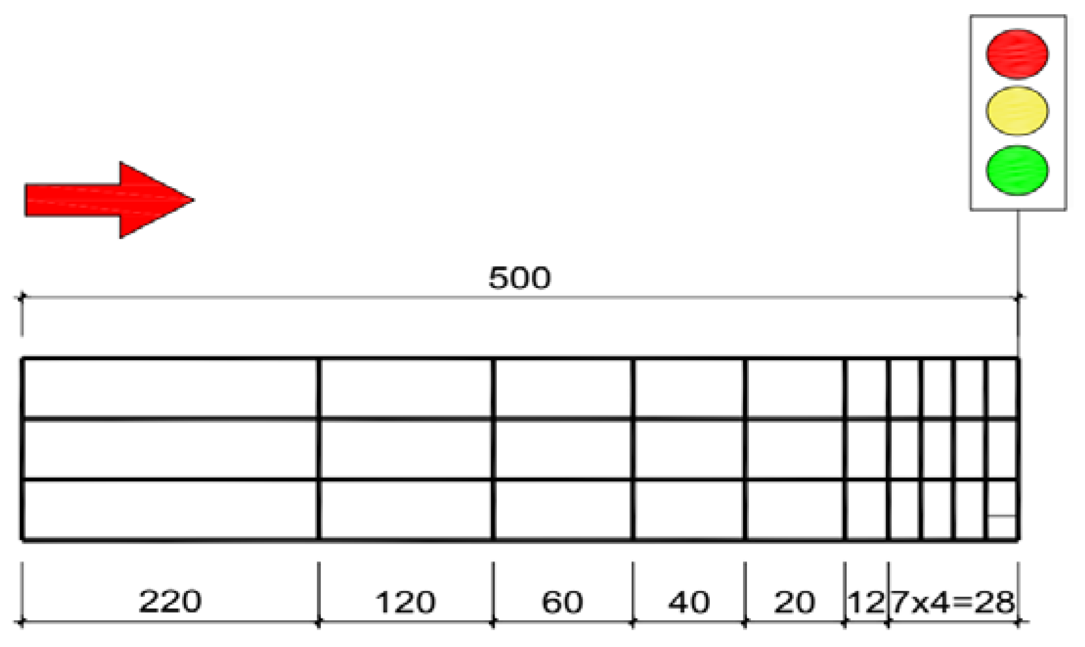
In this study, we used a DRL-based approach to optimize traffic signals by minimizing the cumulative waiting time of all vehicles. The design of the controller involves three aspects: the traffic state space, the traffic signal timing (action space), and the reward. This deep Q-learning combines two aspects of reinforcement learning, DNN and Q-learning, as shown in Figure 6. Because the state space is large, DNN was used to approximate the Q-learning function.

3.2.1. State Space

The state of the agent is used to represent a description of the environment at a given time t and is usually denoted with $s_t$. This state needs to provide sufficient information about the vehicle distribution on each approach so that the agent can learn effectively to optimize traffic.

In this model, we applied the Discrete Traffic State Encoding (DTSE) [52] with a small adjustment to show the state space, inspired by an advanced technique in computing the discretization and quantization of elements. The model used a partially observed environment with data collected only from platoon vehicles (CVs). The whole incoming lane is divided into small cells from the stop line. The length of each cell c will affect the behavior of the model. If this length c is many times larger than the average car length, the individual vehicle dynamics may be lost. However, if this length is too small, it will increase the computational cost, leading to unnecessary complexity. The value in each cell is a binary value used to represent the presence or absence of vehicles in its cell.

Based on this approach, we divided the segment from the starting point to the stop line into cells to discretize the traffic scene. The closer to the intersection, the smaller the width of the cells because it provides important information about the vehicle’s state. The further away from the intersection, the larger the cell size, so as to reduce the amount of computation. There were 30 cells between the beginning of the road and the stop line of the intersection on each approach, as shown in Figure 7. Therefore, there were 120 cells in the whole intersection of different sizes.

The model includes 2 types of vehicles: CVs and RVs. Depending on the operating modes, CVs include leader, follower, catch-up, catch-up follower, and waiting modes. Each cell in the state presentations only contains information about platooning vehicles (CVs) as shown in Figure 8. Based on CV presence, it has a binary value of 0 or 1. Many vehicles can be in a single cell, but the value of that cell is still only 1. In this model, the state description includes the following information: the number of CVs in each direction, CV position (distance to the intersection and lane position), and signal timing information.

The state of the agent at time t can be expressed as St ∈ S. With this state-space definition, the input data are taken from the Sumo simulation to the controller.

3.2.2. Action Space

The purpose of the controller is to find the optimal strategy to reduce the waiting time of all vehicles at the intersection. In this model, the performance of the traffic light system is the action, and we need to define these actions. Collision-free movements are performed in each phase.

The traffic light cycle at this intersection includes red, green, and yellow time. The actions of agents are determined based on the green time from all directions. The action space consists of 4 phases, as shown in Figure 5.

At each time step t, the agent can select one of the possible actions in the action space (a∈A) to take. If the action implemented at time t is the same as the action performed at time t − 1, the green time of this phase is extended. Conversely, if the current action is different from the previous action, the signal light will change to yellow time and take another action. At this time, information and data will be collected and processed. The green time can be different for each action because it depends on the state of each action.

3.2.3. Reward Definition

A reward is an important part of reinforcement learning because it determines the goal of the model after training. In reinforcement learning, after the agent performs an action a in state s, it obtains a reward r from the environment. Through the reward, the agent understands the result of the action and improves the model for the next action choices.

Our main goal in this model is to optimize traffic signals and increase the operational efficiency of the intersection. In our case, we define the reward based on the change in the cumulative waiting time of all vehicles. The waiting time of each vehicle is recorded when the vehicle speed is below or equal to 0.1 m/s before the intersection. The agent will observe all vehicles twice in a green time interval to sum up the cumulative waiting time. The first observed is the beginning of the green phase, and the second is the end of the green phase.

Let $w_{i,t}$ denote the waiting time of the ith observed vehicle when this vehicle enters the model to the beginning of the green time. Moreover, $w{\prime }_{i,t}$ is the waiting time of this vehicle when it enters the model to the end of the green time interval. The equation to determine the cumulative waiting time of all vehicles at the beginning and the end of each phase is as follows:

$${\mathrm{W}}_{\mathrm{t}} = {\displaystyle \sum _{\mathrm{i} = 1}^{\mathrm{N}}{\mathrm{w}}_{\mathrm{i}, \mathrm{t}}} \mathrm{a}\mathrm{n}\mathrm{d} {{\mathrm{W}}^{\prime }}_{\mathrm{t}} = {\displaystyle \sum _{\mathrm{i} = 1}^{\mathrm{N}}{{\mathrm{w}}^{\prime }}_{\mathrm{i}, \mathrm{t}}}$$

(6)

If the vehicle speed is greater than 0.1 m/s, its waiting time is over, and it is not added to the cumulative time. Since our aim is to increase the efficiency of the intersection, the model reward is based on the reduction in total cumulative waiting time. The reward function in our model is shown below:

$${\mathrm{r}}_{\mathrm{t}} = {\mathrm{W}}_{\mathrm{t}} - {{\mathrm{W}}^{\prime }}_{\mathrm{t}}$$

(7)

In this model, the reward is a negative cumulative waiting time, because the cumulative waiting time of all vehicles at the end of the green time will be greater than the cumulative waiting time of all vehicles at the beginning of the green time. Moreover, the agent will choose the appropriate actions (changing the duration of green time and the phase order) to minimize the cumulative waiting time.

3.2.4. Parameters of the Training Process

• Activation functions

The activation function in a deep neural network plays an important role in the operation of the training process. It determines how the weighted sum is transformed into an output from input layers. In our model, we used a rectified linear unit (ReLU) to output the results.

$$\mathrm{f} (\mathrm{x}) = \{\begin{array}{l} 0 \mathrm{f}\mathrm{o}\mathrm{r} \mathrm{x} < 0\\ \mathrm{x} \mathrm{f}\mathrm{o}\mathrm{r} \mathrm{x} \ge 0\end{array}$$

(8)

• Optimization function

We used adaptive moment estimation (Adam) for training optimization in DNN. This algorithm is used for the first-order gradient-based optimization of the stochastic objective function [53]. This method is easy to implement, has high computational efficiency, requires little memory, and is suitable for models with large amounts of data.

• Experience replay

Experience replay is a replay memory technique used in DNN to improve the performance of the agent. In this method, we stored randomly the information needed for training in groups of samples called batches. The experiences of the agent at each time step are stored in samples as

$$\mathrm{m}=\left\{ {\mathrm{s}}_{\mathrm{t}}, {\mathrm{a}}_{\mathrm{t}}, {\mathrm{r}}_{\mathrm{t}+1}, {\mathrm{s}}_{\mathrm{t}+1}\right\}$$

(9)

where $r_t$ is the reward when the agent performs the action in the state $s_t$ and causes the environment to change to a new state, $s_{t+1}$. This technique is used to solve the autocorrelation that renders the model unstable when training, since $s_{t+1}$ is directly evolved from $s_t$.

This technique needs to specify the memory and batch size. The memory size is defined as the maximum number of samples that can be stored. In this model, we set the maximum memory size to 50,000 samples. The batch size indicates the number of samples taken from memory for each training iteration and is set to 100. If the memory is full, the oldest sample is removed, and the new sample is inserted.

• Epsilon in Q-Learning Policy

In this paper, we use the epsilon (ε) greedy policy to balance exploration and exploitation. Here, ε is the trade-off between exploration and exploitation, and it refers to the agent’s probability of exploration when choosing an action. The equation for ε decay by episode is as follows:

$$\mathsf{\epsilon } = 1 - \frac{\mathrm{C}\mathrm{u}\mathrm{r}\mathrm{r}\mathrm{e}\mathrm{n}\mathrm{t}\_\mathrm{e}\mathrm{p}\mathrm{i}\mathrm{s}\mathrm{o}\mathrm{d}\mathrm{e}\mathrm{s}}{\mathrm{T}\mathrm{o}\mathrm{t}\mathrm{a}\mathrm{l}\_\mathrm{e}\mathrm{p}\mathrm{i}\mathrm{s}\mathrm{o}\mathrm{d}\mathrm{e}\mathrm{s}}$$

(10)

All Q values are updated iteratively during the training of the agent. At the initial time, ε = 1, meaning that the agent completely explores the environment. The more an agent explores the environment, the more it understands the environment. ε gradually decays during training, and the agent will exploit more than explore. Based on the learned experience, the agent understands the environment more and will exploit more. In the last episode, ε = 0, and the agent fully exploits based on trained knowledge about the environment.

3.2.5. Determine the Hyperparameters

Hyperparameters are parameters used to control the learning process in DNN. Their values need to be determined before starting the learning process. These hyperparameters affect the output of the model. There are no specific rules for choosing the number of neurons or the number of hidden layers. The selection of too many layers or neurons causes the model over-fitting and increases the time to train the model. Conversely, choosing too few layers or neurons causes model under-fitting and high statistical bias. In this work, we performed trial and error tests to determine the hyperparameters by changing the number of hidden layers and neurons.

We first created three models with 2, 4, and 8 hidden layers, respectively, to determine the number of hidden layers that fit the model. In the case of a platoon with three vehicles, the results of these models are shown in

Table 2. Hyperparameters of DNN.

Parameter	Cumulative Negative Reward (s)	Cumulative Delay Time (s)
Hidden layers = 2, Neurons = 128	−9947	25,677
Hidden layers = 4, Neurons = 128	−10,671	28,115
Hidden layers = 8, Neurons = 128	−11,974	29,652
Hidden layers = 2, Neurons = 256	−12,824	30,235
Hidden layers = 2, Neurons = 512	−11,508	30,654

.

We can see that the model performance decreased when increasing the number of hidden layers. The cumulative negative reward (total waiting time) of vehicles was reduced from 11,974 s to 9947 s when changing the number of hidden layers from 8 to 2. The model with two hidden layers gave the best results, and we chose this number of hidden layers for the next steps. Next, we changed the number of neurons on hidden layers between 128, 256, and 512. When we decreased the number of neurons on hidden layers from 512 to 128, the total waiting time was reduced by 15%. Having too many neurons is undesirable, but the model needs to have enough neurons to be able to acquire the complexities of the input–output relationship. We performed the same steps to determine other hyperparameters in the model to obtain the optimal model. The final structure of the DNN and agent parameters are shown in

Table 3. Parameters of agent.

Parameter	Value
Gui	False
Total Episode	300
Max_steps	3600 s
Green duration	5 s
Yellow duration	3 s
Learning rate	0.001
Batch_size	100
Training_epochs	800
Num_states	120
Num_actions	4
gama	0.75

and

Table 4. Structure of neural network.

Parameter	Value
Simulator	SUMO
Num_layers (Hidden layers)	2
Width_layers (Neurons)	256
Loss Function	Mean Squared Error
Activation Function	Relu
Optimization Function	Adam Optimizer

.

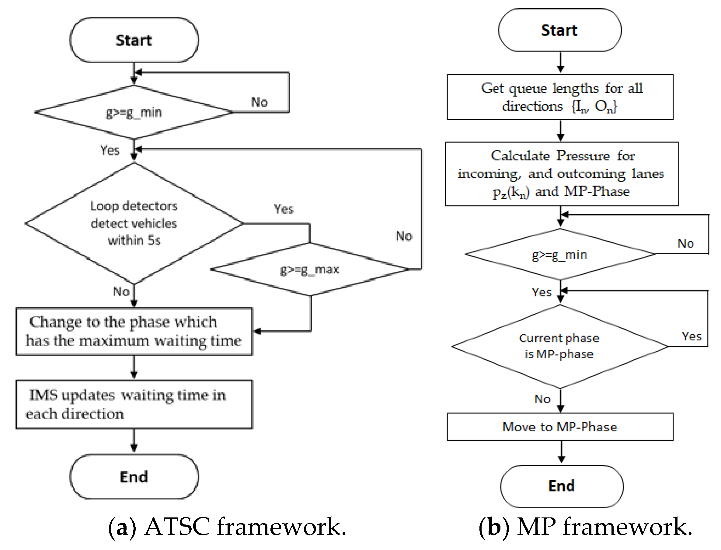
3.3. Scenario 2: ATSC-Based Scenario at the Signalized Intersection

The flow chart of the ATSC scenario is shown in part a) of Figure 9. In this model, we used 12 loop detectors to detect all vehicles (CVs and RVs) when passing them. Loop detectors were permanently mounted on the road and measured the traffic flow through them. Based on the collected information, the IMS adjusted the green time of traffic signals according to the set rules. The green time of each phase needed to be greater than the minimum green time (10 s) before switching to another phase. In any green phase, if the loop detector detected vehicles within 5 s, the green time of this phase was extended by ${\mathsf{\Delta }}_t$ (s) to ensure that the platoon had enough time to cross the intersection without waiting. If vehicles were not detected within 5 s, the green phase ended and switched to another phase that had the maximum waiting time. The duration of green time changed continuously depending on the traffic approaching the intersection. The minimum green time for each phase was 10 s, and the maximum was 45 s.

Based on the communication, the IMS obtained the speed and time interval of all vehicles. The waiting time of each vehicle was recorded when the vehicle speed was below or equal to 0.1 m/s before the intersection. Moreover, the IMS determined the waiting times of all vehicles and the cumulative waiting time of each phase. The selected green phase had the maximum waiting time. After each cycle ends, the IMS updated the waiting time of each direction to select the next green phase.

3.4. Scenario 3: MP-Based Scenario at the Signalized Intersection

For comparison, we implemented another scenario of intersection management based on max pressure (MP), as shown in part (b) of Figure 9. This was a feedback-based signal control algorithm that stabilized the queue length and maximized throughput. This controller did not need to know about the current or future traffic volume of the network. It only required the real-time measurement of the queue length in all directions to and from the intersection. The signal control plan consisted of 4 phases with duration based on the MP algorithm.

In this scenario, 24 area detectors were placed in 24 lanes to and from the intersection to measure the queue length per lane. The intersection (n) is presented as a graph with links $\mathrm{z} \in$ Z, including the incoming link set (I_n) and outgoing link set (O_n).

The equation that describes the evolution of queue length for link z is expressed as follows:

$${\mathrm{x}}_{\mathrm{z}} ( \mathrm{t} + 1 )= {\mathrm{x}}_{\mathrm{z}} (\mathrm{t}) + {\mathrm{T}}_{\mathrm{t} \to (\mathrm{t}+1)} [ {\mathrm{q}}_{\mathrm{z}} (\mathrm{t}) -{\mathrm{s}}_{\mathrm{z}} (\mathrm{t}) + {\mathrm{d}}_{\mathrm{z}} (\mathrm{t}) -{\mathrm{u}}_{\mathrm{z}} (\mathrm{t})]$$

(11)

Here,

• ${\mathrm{x}}_{\mathrm{z}} (\mathrm{t})$ is the number of vehicles in link z to link m at the end of the discrete-time t.
• ${\mathrm{q}}_{\mathrm{z}} (\mathrm{t}) \mathrm{a}\mathrm{n}\mathrm{d} {\mathrm{u}}_{\mathrm{z}} (\mathrm{t})$ are the inflow and outflow in the same period.
• ${\mathrm{d}}_{\mathrm{z}} (\mathrm{t}) \mathrm{a}\mathrm{n}\mathrm{d} {\mathrm{s}}_{\mathrm{z}} (\mathrm{t})$ are the demand and saturation flow in this link.

The state x_z (k_n) of each link is determined based on the number of vehicles in the queue length according to real-time measurement. The pressure of this link can be calculated as follows:

$${\mathrm{p}}_{\mathrm{z}} ({\mathrm{k}}_{\mathrm{n}}) = \left[\frac{{\mathrm{x}}_{\mathrm{z}} ({\mathrm{k}}_{\mathrm{n}})}{{\mathrm{x}}_{\mathrm{z}, \max }} - {\displaystyle \sum _{\mathrm{w} \in {\mathrm{O}}_{\mathrm{n}}}\frac{{\mathsf{\beta }}_{\mathrm{i}, \mathrm{w} }{\mathrm{x}}_{\mathrm{w}} ({\mathrm{k}}_{\mathrm{n}})}{{\mathrm{x}}_{\mathrm{w}, \max }} {\mathrm{g}}_{\mathrm{n}, \mathrm{j}}} ({\mathrm{k}}_{\mathrm{n}})\right] {\mathrm{S}}_{\mathrm{z}}$$

(12)

Here,

• ${\mathrm{x}}_{\mathrm{z}, \max } \mathrm{a}\mathrm{n}\mathrm{d} {\mathrm{x}}_{\mathrm{w}, \max }$ are the storage capacity of link z and link w.
• ${\mathsf{\beta }}_{\mathrm{i}, \mathrm{w} }$ is the turning movement rate with $\mathrm{i} \in {\mathrm{I}}_{\mathrm{n}}$ and $\mathrm{w} \in {\mathrm{O}}_{\mathrm{n}}$.
• ${\mathrm{k}}_{\mathrm{n}}$ is the control discrete time index.
• ${\mathrm{g}}_{\mathrm{n},\mathrm{j}}$ is the green time of stage j.

Pressure in each direction is defined as the difference between the upstream and downstream queue length. In this case, the output links are exiting links with infinite capacity, and the second term in Equation (12) becomes zero. Thus, the pressure of each link is simply equal to the queue length multiplied by the saturation ratio ($S_z$). The pressure of each stage j of the intersection can be determined as

$${\mathrm{P}}_{\mathrm{n},\mathrm{j}} ( {\mathrm{k}}_{\mathrm{n}}) = \max \left\{ 0, {\displaystyle \sum _{\mathrm{z} \in {\mathrm{v}}_{\mathrm{j}} }{\mathrm{p}}_{\mathrm{z}} ({\mathrm{k}}_{\mathrm{n}})}\right\}$$

(13)

The total effective green time for intersection n (${\mathrm{G}}_{\mathrm{n}}$) could be obtained by

$${\mathrm{G}}_{\mathrm{n}} = {\mathrm{C}}_{\mathrm{n}} - {\mathrm{L}}_{\mathrm{n}} - {\displaystyle \sum _{\mathrm{j} \in {\mathrm{F}}_{\mathrm{n}}}{\mathrm{g}}_{\mathrm{n}, \mathrm{j}, \min } \mathrm{w}\mathrm{i}\mathrm{t}\mathrm{h} \mathrm{n}\in \mathrm{N}}$$

(14)

${\mathrm{g}}_{\mathrm{n}, \mathrm{j}, \min }$ is the minimum green time for stage j of intersection n. This value is taken in the ATSC-based scenario as 10 s. Moreover, ${\mathrm{g}}_{\mathrm{n}, \mathrm{j}} ( {\mathrm{k}}_{\mathrm{n}})$ is the green time spent in phase j with the constraint

$${\mathrm{g}}_{\mathrm{n}, \mathrm{j}} ( {\mathrm{k}}_{\mathrm{n}}) \ge {\mathrm{g}}_{\mathrm{n}, \mathrm{j}, \min }$$

(15)

The number of vehicles in the queue length at each lane was extracted from the 24 area detectors on each lane. Based on the collected data, the IMS continuously calculated the pressure for the 4 phases and determined the stage with MP. After the minimum green time of the current phase has expired, the IMS checked whether the current phase has maximum pressure. If the current phase was the MP phase, the IMS prolonged the current phase until the other phase had MP. Conversely, if the current phase was not the MP phase, then the IMS shifted the current phase to the MP phase. The IMS continuously updated the pressure of each stage to control the intersection.

3.5. Performance Evaluation Metric

A reinforcement learning algorithm is measured by the reward received during the learning process [54]. During the simulation, the agent tries to maximize the reward. A better-trained DRL model gets more reward value. The cumulative reward curve from 300 random runs was measured and evaluated to evaluate the trained model. Finally, we compared our algorithm results with other benchmark tasks for average delay time, waiting time, speed, and CO₂ emissions. These are the common metrics used to evaluate traffic performance [55].

4. Results and Evaluation

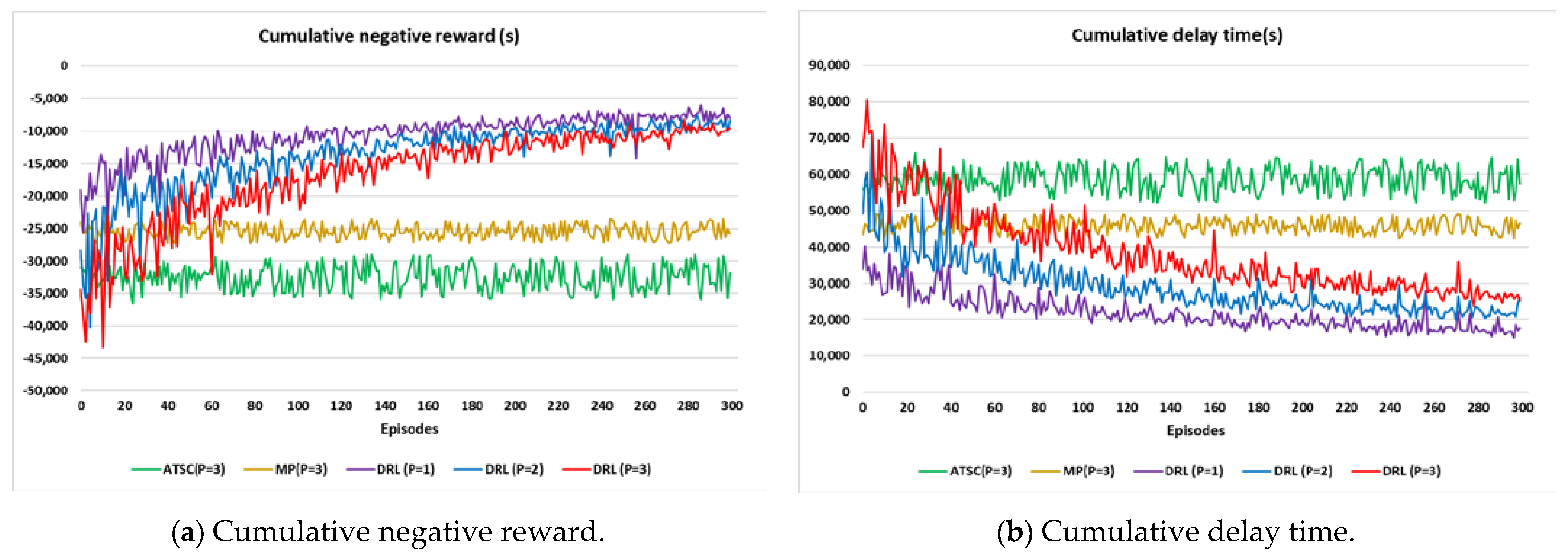
4.1. Performance of DRL, ATSC, and MP-Based Models

The cumulative negative reward (cumulative waiting time) and delay time were used to evaluate the effectiveness of the DNN model. The simulated results are shown in Figure 10 below.

Through the learning process, the cumulative negative reward approached zero, which means that the total waiting time of all vehicles decreased, and the agent learned gradually. Although the reward line fluctuated, its overall trend was upward. At the beginning of training, this curve oscillated with a large amplitude but then gradually decreased. It can be seen that after the training process, the cumulative waiting time of all vehicles decreased by around 70% compared to that before training. The model results show that the cumulative reward was increased from around −35,000 s, −28,000 s, and −20,000 s to around −9600 s, −11,200 s, and −8000 s, respectively, for the cases of platoons consisting of 3, 2, and 1 vehicles. The cumulative waiting time of all vehicles passing through the intersection decreased, so the cumulative delay time also decreased, as expressed in part (b) of Figure 10. This result proved that the model was efficient, and it was implemented in the next steps. In the early episodes, the epsilon rate (in Equation (10)) was high, and the agent did not fully explore the action and state space. Therefore, the total cumulative time of this model was larger than in the ATSC- and MP-based scenarios. As the model continued to learn, the epsilon was gradually reduced, and the agent concentrated on exploiting the optimal policy from the previous episodes for higher rewards. And the models also gradually converged when the reward curve was unchanged. Finally, the total cumulative waiting time of the DRL-based scenario was 50% and 65% better than that of the MP- and ATST-based scenarios for platoons with three vehicles.

However, as the number of episodes increased, the total wait time in the ATSC- and MP-based scenarios did not change significantly because the intersection traffic management in the two scenarios was based on the pre-defined algorithm without “learning”. These two scenarios have the same characteristics: (a) 4 phases to separate the queue length in all movements; (b) the assumption of queue length with unbounded capacities on all links; (c) the traffic controller without a fixed cycle and cyclic phases. The cumulative waiting time of the MP- and ATSC-based scenarios fluctuated around 25,000 and 32,000 s. The performance difference can be explained through the intersection traffic controller. The algorithm in the MP-based scenario prevented any queue length from growing indefinitely and created a stable intersection with a suitable queue length. The MP-based scenario had better performance than ATSCT because it gave priority to stabilizing the queue length. This algorithm reduces the pressure at the intersection reasonably, whereas the traffic controller in the ATSC-based scenario manages the intersection based on the sensor’s vehicle detection. It prolongs the green time for the high-traffic directions but also increases the queue length in other directions. Therefore, the green time duration in the ATSC method was large than that in the MP method. Finally, it achieves worse results, but the difference between the ATSC- and MP-based scenarios is not large (20%).

Another important finding was the influence of traffic flow rates on these models. Vehicles arrived at the intersection independently when traffic flow was low (platoon_size = 1). When CVs arrived, the signal agent quickly changed phase to ensure the minimum waiting time; and for RVs, the traffic signal did nothing. Since all vehicles arrived individually, the agent handled the vehicles separately.

When the traffic volume is higher (platoon_size = 3), vehicles that arrived at the intersection followed the flow of traffic, not independently. Since the traffic agent cannot pay attention to only each CVs, the agent optimized the waiting time for the whole vehicle.

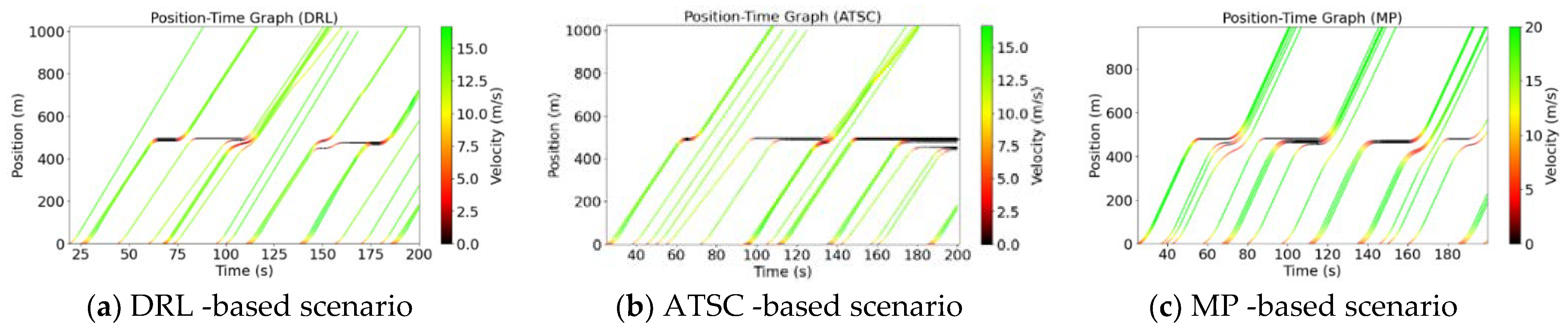
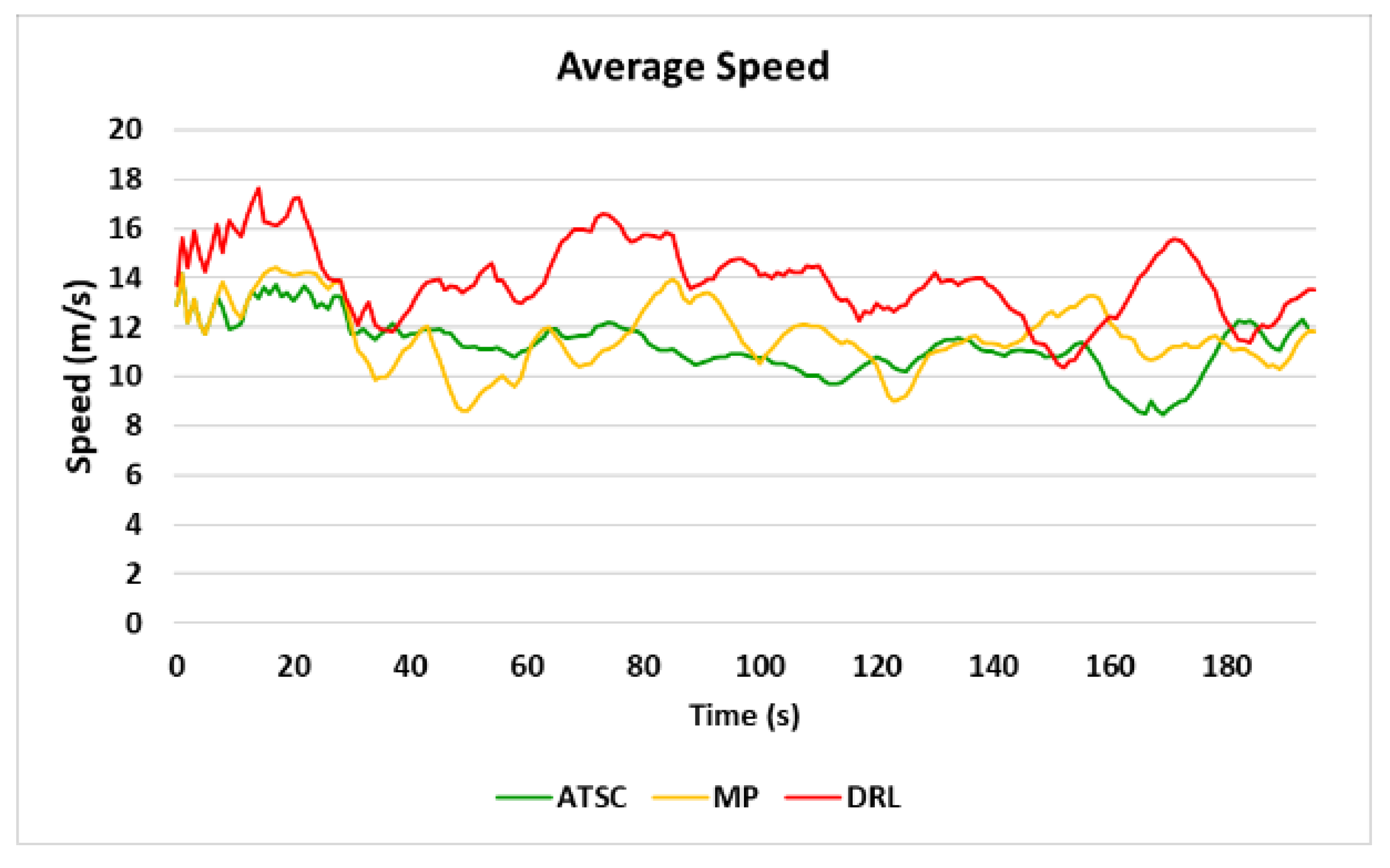
4.2. Trajectories and Average Speed of 3 Scenarios

In this section, we present graphs demonstrating the position and average speed over time for the 3 scenarios, DRL, ACTS, and MP, for the case of a platoon consisting of 3 vehicles.

The distance–time relationship between vehicles from west to east for one lane in 200 s is plotted in Figure 11. Colors in the graphs show the speed of the vehicles when moving, in which green corresponds to the highest speed (20 m/s) and black corresponds to the lowest speed (0 m/s). Alternatively, one can perceive the vehicle’s speed adjustment based on the slope of these lines. Platoons started at 5 m/s (starting speed of vehicles when entering the model) and then increased to the desired speed. When approaching the intersection, if the light was green, vehicles kept moving and passed the intersection. If the light was red, vehicles had to stop and wait until the light was green to pass. After passing the intersection, platoons moved at the desired speed. The green time duration depends on the algorithm applied in each scenario.

It can be seen that the green time in the ATSC-based scenario tends to be longer than in the DNN- and MP-based scenarios. In this scenario, the green light phase depends on the sensor’s vehicle detection. If vehicles are still detected, the green light will be extended until the maximum limit or no more vehicles are detected. In contrast to ATSC, the MP controller is stable in terms of queue length, so it quickly changes phase when detecting a larger pressure in the other direction. Therefore, the length of the green phase in this scenario is shorter. The DRL-based scenario has the most reasonable green time compared to the two aforementioned scenarios. After learning, the traffic agent optimized the intersection’s green time and cycle length. Although the traffic light duration is variable, the trained model can handle this uncertainty.

The average speed graph of the three scenarios is also expressed in Figure 12. The average speed of scenarios decreases when many cars must wait in line at the intersection. With a shorter red and green duration, the model efficiency is improved, and the vehicle speed is also greater. The speed perturbation is amplified by the RVs between platoons and reduced by the platooned vehicles. The DRL-based scenario optimizes the waiting time, so all vehicles (CVs and RVs) move at the highest speed. We can see that this average velocity is cyclic with traffic signals and peaks at the middle of the green phases. With the current traffic demand, the average speed of the DRL-based scenario is larger than in the other two scenarios, but this difference is not significant (approximately 10%).

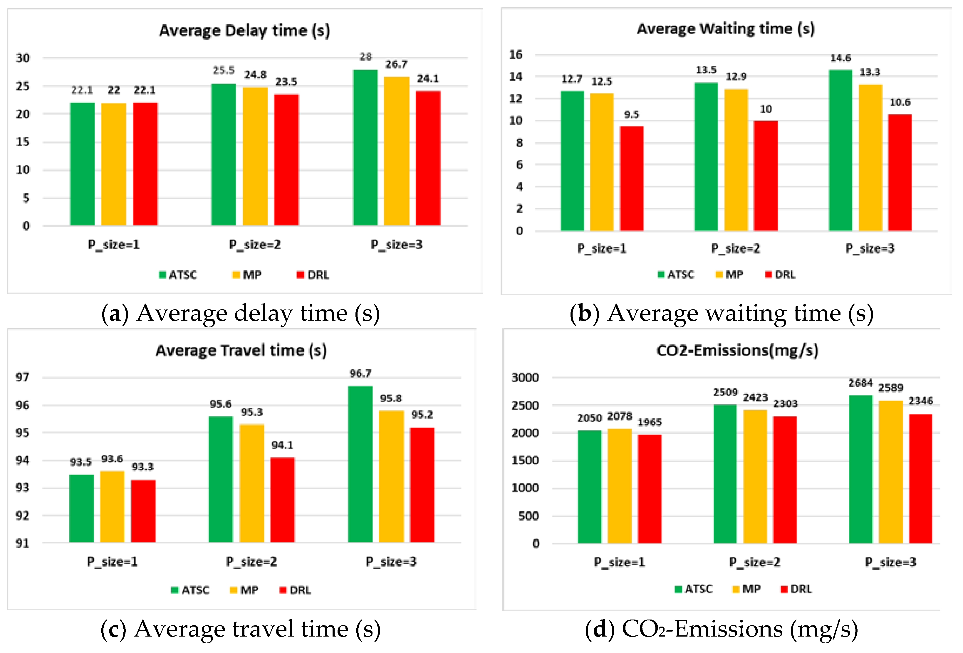
4.3. MOE Performance

We evaluated the traffic performance of the three scenarios with the following criteria: average delay time, waiting time, travel time, and CO₂ emissions. Results are shown in Figure 13 below.

The MOE evaluation showed that the traffic management policy was the most important aspect that affected the model performance. The DRL-based scenario had the best results (average delay times were 24.1, 23.5 s, and 22.1 s, corresponding to 3, 2, and 1 vehicles in a platoon). It is 10% and 13% smaller than the MP- and ATSC-based scenarios, as presented in part a) of Figure 13. This result proves the superiority of the trained model compared to the other two models.

The waiting time of the 3 scenarios is shown in part (b) of Figure 13. The DRL-based scenario had considerably higher performance, with an average waiting time of 10.6 s, because it reached the maximum cumulative reward, as mentioned in Figure 10. Compared with the ATSC- and MP-based scenarios, the average waiting time of vehicles in the DRL-based scenario was improved by 20% and 28%, respectively (in the case of a platoon having 3 vehicles).

Part (c) and (d) of Figure 13 show that the DRL-based policy was better than other policies in terms of travel time and CO₂ emissions. However, the difference between these policies was not large. The minimum travel time was 95.2 s for the DRL-based scenario, and the longest travel time was 96.7 s for the ATSC-based scenario, with a difference of 4% (in the case of a platoon having 3 vehicles).

Between these scenarios, the DRL-based scenario had the smallest CO₂ emissions (2346 mg/s) for the case with 3 vehicles in one platoon. The MP-based scenarios were slightly better than the ATSC method. The three scenarios improved the traffic efficiency; thus, the CO₂ emissions were improved further. However, the degree of improvement in each scenario varied based on the performance of the vehicles.

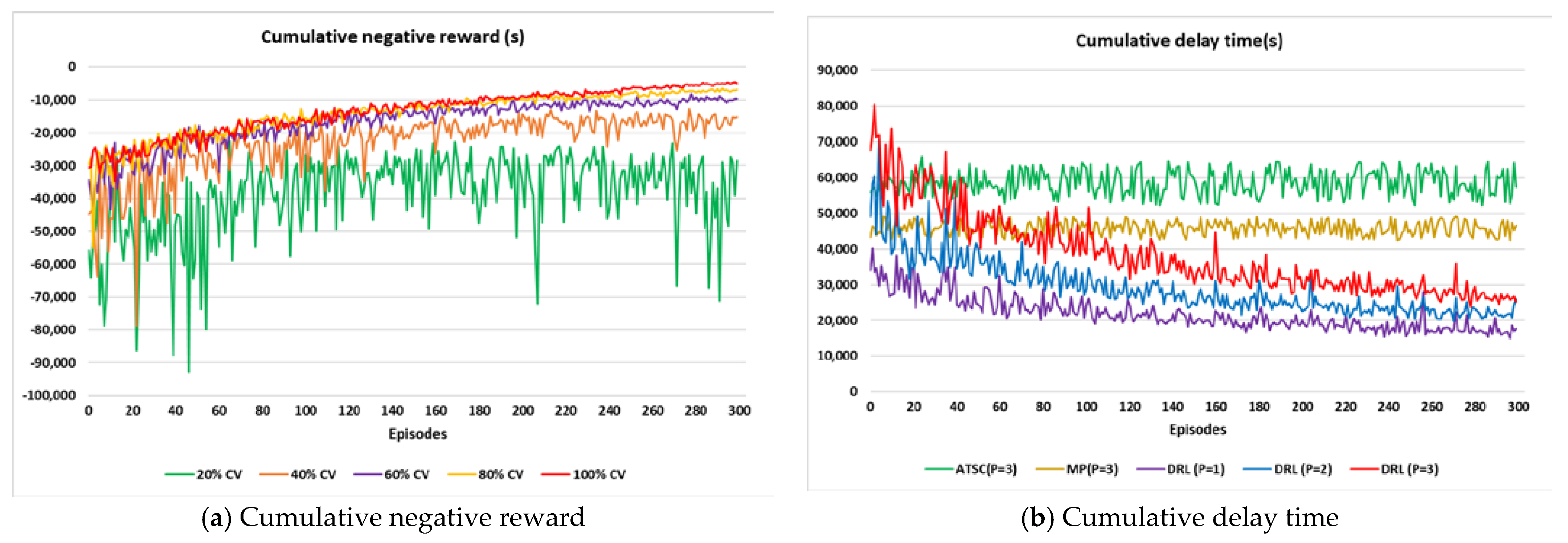
4.4. Effect of Penetration Rate

To evaluate the effect of CV agents, models were implemented with variable penetration rates. We compared 5 scenarios with penetration rates of 20%, 40%, 60%, and 80%, respectively, and with a platoon of size 3. The input flow and model results are shown in

Table 5. Traffic simulation results with different CV penetration rates.

CV Penetration Rate	Platoons (Size = 3)	RVs	Cumulative Negative Reward	Average Speed (m/s)	Average Waiting Time (s)	Average Delay Time (s)
20%	160	1920	−28,529	8.8	35.8	61.6
40%	320	1440	−15,144	10.19	18.8	35.2
60%	480	960	−9603	11.2	10.6	24.1
80%	640	480	−6987	11.7	8.0	21.2
1000%	800	0	−4886	12.1	5.6	19.0

.

The cumulative negative reward and delay time in the learning process is shown in Figure 14 below.

From Figure 14, it can be seen that when the CV penetration rate increases, the efficiency of the DQN model is improved. However, this improvement is only achieved when CV penetration is at a significant level. The model’s improvement is quite insignificant when the CV penetration rate is low. Because at this rate, the amount of information collected is not enough for the learning process. The model is only truly improved when the CV penetration rate is greater than 20%. With a high degree of penetration, platoons can merge into longer platoons during movement or at an intersection area. This will improve the model significantly in terms of both throughput and waiting time.

In addition, when the CV penetration rate is low, the fluctuation degree of the reward curve is large. At a rate of 20%, although the cumulative negative reward curve seems to converge, the reward fluctuates between −30,000 s and −50,000 s, which is very unstable. As the CV rate increases, this fluctuation also decreases. It is clear that the higher the CV rate, the more data the agent gets in each episode, improving the learning model’s efficiency. The model is the most effective when the CV penetration rate is 100%, i.e., all vehicles in the model are CVs. With this rate, the model efficiency is improved more than 6 times compared to the scenario with a 20% penetration rate.

5. Discussion

In this paper, we proposed a deep reinforcement learning method having vehicle platooning at an isolated signalized intersection with partial detection. Other papers often assume that all vehicles are detected to collect data. This is not true because only vehicles equipped with a wireless communication system can be connected. In addition, our study considered the formation of platoons between CVs of different sizes.

After the training, the cumulative waiting time of all vehicles decreased by around 70% compared to that before the training. Through the learning process, the agent learned gradually, and the total waiting time of all vehicles decreased. It is 50% and 65% better than that of the MP and ATST-based scenarios for platoons with three vehicles. The results of this paper demonstrated the advantage of applying DRL in traffic management, similar to other papers [20,36,47].

However, our model combines DRL with platoon formation, so the results are much improved compared to that of other papers. Compared with the cumulative reward curve in [36], our model has higher stability with small fluctuations. Because the platoon formation changed the behavior and characteristics of car-following models and affected overall traffic performance. It makes traffic flow stable with a lower waiting time. This is also shown at the beginning of the learning process, the waiting time in our model also has a smaller value.

Simulation results have shown that the DRL-based intersection management method is the most effective. Compared with the ATSC- and MP-based scenarios, the average waiting time of vehicles in the DRL-based scenario was improved by 20% and 28%, respectively (in the case of a platoon having three vehicles). Therefore, other metrics, such as delay time, travel time, and CO₂ emissions, were also reduced compared to other policies. The DRL-based intersection management policy has also proven its effectiveness.

Our model also shows that as the CV penetration rate increases, traffic efficiency also improves. At a rate of 20%, although the cumulative negative reward curve seems to converge, the reward fluctuates between −30,000 s and −50,000 s, which is very unstable. The model is only truly improved when the CV penetration rate is greater than 20%. As the CV penetration rate is higher, the model performance is further improved, further reducing the waiting times of all vehicles. This was also demonstrated in several papers on the influence of CV penetration rates on traffic efficiency [39,46].

Platoon size is an important factor in the traffic model. The simulation model also tested the influence of the number of vehicles in the platoon. As the number of vehicles in the platoon increases, the model’s stability also reduces. The delay time increases by 7% and 10% when the number of vehicles in the platoon increases from 1 to 2 and 3 vehicles. Therefore, an appropriate platoon size may be more suitable in urban areas because it could dampen perturbance better.

We assumed the models perform under ideal conditions and perfect communication between CVs. So, there was no damage, data package loss, or time delay during the transmission. In addition, we did not consider the influence of other modes such as buses, bicycles, or pedestrians. There were only two types of vehicles in our model (CVs and RVs). Therefore, to implement the model in practice, it is necessary to add more factors to the model.

Although this approach has been successful for an isolated signalized intersection, many problems need to be addressed when applying the model to multi-intersection networks. Many agents (intersections) learn simultaneously to solve a task by interacting with the same environment in a road network. The algorithm, in this case, is more complex than the one we used in this study. An action performed by a particular agent can achieve different rewards depending on the actions performed by other agents. In addition, we need to model the interaction between agents and how they share information with each other.

6. Conclusions

In this paper, we have presented three intersection management policies (DRL, ATSC, and MP) in mixed traffic flow (CVs and RVs) with partial detection. In these scenarios, it was assumed that the wireless communication between platooned vehicles was perfect. The deep Q-learning model combines two aspects of reinforcement learning, DNN and Q-learning. Our main goal in this model is to optimize traffic signals and to reduce the waiting time of all vehicles. There are two types of vehicles in our model. Platooning vehicles are detected vehicles, and RVs are undetected vehicles. The model only collects data on detected vehicles (CVs) during training.

Our contribution is to combine DRL and platoon formation to improve traffic efficiency in urban environments with different CV penetration rates. Therefore, traffic management agencies can apply this proposed approach to reduce waiting time at signalized intersections.

To compare the effectiveness of the proposed model, we implemented two benchmark methods, ATSC and MP. These three scenarios were simulated at a signalized intersection to measure traffic metrics (waiting time, delay time, travel time, speed, and CO₂ emissions). In addition, the model also tested the influence of the platoon by changing the number of vehicles in the platoon.

In addition, platoon formation increases model efficiency and reduces the fluctuation of the reward during training. This is a very promising result in the future when the CV penetration rate is high. Experimental results in three scenarios (DRL, ATSC, and MP) with different CV penetration rates prove that DRL can handle all kinds of traffic. Although the results are different for each optimization scenario, DRL is a promising solution to apply to the overall optimization scheme.

In this paper, we introduced a traffic simulation model for an isolated signalized intersection (single agent), and we believe that this could be applied to multi-agent scenarios to coordinate traffic lights. In the future, we plan to study complex road networks with many traffic signal phases and real traffic data in different ways (centralized and decentralized). In addition, we will devise a scenario that combines both signalized intersections and unsignalized intersections with different scenarios.

References

1. Howie, D. Urban traffic congestion: A search for new solutions. ITE J. 1989, 59, 13–16. [Google Scholar]
2. Bivina, G.R.; Landge, V.; Kumar, V.S. Socio economic valuation of traffic delays. Transp. Res. Procedia 2016, 17, 513–520. [Google Scholar] [CrossRef]
3. Hofer, C.; Jager, G.; Fullsack, M. Large scale simulation of CO2 emissions caused by urban car traffic: An agent-based network approach. J. Clean. Prod. 2018, 183, 1–10. [Google Scholar] [CrossRef]
4. Dey, K.C.; Rayamajhi, A.; Chowdhury, M.; Bhavsar, P.; Martin, J. Vehicle-to-vehicle (V2V) and vehicle-to-infrastructure (V2I) communication in a heterogeneous wireless network—Performance evaluation. Transp. Res. Part C Emerg. Technol. 2016, 68, 168–184. [Google Scholar] [CrossRef] [Green Version]
5. Chen, L.; Englund, C. Cooperative intersection management: A survey. IEEE Trans. Intell. Transp. Syst. 2016, 17, 570–586. [Google Scholar] [CrossRef]
6. Kuang, X.; Zhao, F.; Hao, H.; Liu, Z. Intelligent connected vehicles: The industrial practices and impacts on automotive value-chains in China. Asia Pac. Bus. Rev. 2017, 24, 1–21. [Google Scholar] [CrossRef]
7. Traub, M.; Maier, A.; Barbehön, K.L. Future automotive architecture and the impact of IT trends. IEEE Softw. 2017, 34, 27–32. [Google Scholar] [CrossRef]
8. Kopelias, P.; Demiridi, E.; Vogiatzis, K.; Skabardonis, A.; Zafiropoulou, V. Connected & autonomous vehicles—Environmental impacts—A review. Sci. Total Environ. 2020, 712, 135237. [Google Scholar]
9. Olia, A.; Razavi, S.; Abdulhai, B.; Abdelgawad, H. Traffic capacity implications of automated vehicles mixed with regular vehicles. J. Intell. Transp. Syst. 2018, 22, 244–262. [Google Scholar] [CrossRef]
10. Chen, L.; Zhang, Y.; Li, K.; Li, Q.; Zheng, Q. Car-following model of connected and autonomous vehicles considering both average headway and electronic throttle angle. Mod. Phys. Lett. B 2021, 35, 2150257. [Google Scholar] [CrossRef]
11. Fu, R.; Li, Z.; Sun, Q.; Wang, C. Human-like car-following model for autonomous vehicles considering the cut-in behavior of other vehicles in mixed traffic. Accid. Anal. Prev. 2019, 132, 105260. [Google Scholar] [CrossRef]
12. Papadoulis, A.; Quddus, M.; Imprialou, M. Evaluating the safety impact of connected and autonomous vehicles on motorways. Accid. Anal. Prev. 2019, 124, 12–22. [Google Scholar] [CrossRef]
13. Liu, H.; Kan, X.; Shladover, S.E.; Lu, X.Y.; Ferlis, R.E. Impact of cooperative adaptive cruise control on multilane freeway merge capacity. J. Intell. Transp. Syst. 2018, 22, 263–275. [Google Scholar] [CrossRef]
14. Zohdy, I.H.; Rakha, H.A. Intersection management via vehicle connectivity: The intersection cooperative adaptive cruise control system concept. J. Intell. Transp. Syst. 2016, 20, 17–32. [Google Scholar] [CrossRef]
15. Van Arem, B.V.; Van Driel, C.J.G.; Visser, R. The impact of cooperative adaptive cruise control on traffic-flow characteristics. IEEE Trans. Intell. Transp. Syst. 2006, 7, 429–436. [Google Scholar] [CrossRef] [Green Version]
16. Segata, M. Platooning in SUMO: An open-source Implementation. In Proceedings of the SUMO User Conference 2017, Berlin, Germany, 8–10 May 2017; pp. 51–62. [Google Scholar]
17. Segata, M.; Joerer, S.; Bloessl, B.; Sommer, C.; Dressler, F.; Cigno, R.L. Plexe: A Platooning Extension for Veins. In Proceedings of the 2014 IEEE Vehicular Networking Conference, Paderborn, Germany, 3–5 December 2014. [Google Scholar]
18. Sturm, T.; Krupitzer, C.; Segata, M.; Becker, C. A Taxonomy of Optimization Factors for Platooning. IEEE Trans. Intell. Transp. Syst. 2021, 22, 6097–6114. [Google Scholar] [CrossRef]
19. Haas, I.; Friedrich, B. An autonomous connected platoon-based system for city-logistics: Development and examination of travel time aspects. Transp. A Transp. Sci. 2018, 17, 151–168. [Google Scholar] [CrossRef]
20. Liang, K.Y.; Martensson, J.; Johansson, K.H. Experiments on Platoon Formation of Heavy Trucks in Traffic. In Proceedings of the 2016 IEEE 19th International Conference on Intelligent Transportation Systems (ITSC), Macau, China, 1–4 November 2016. [Google Scholar]
21. Maiti, S.; Winter, S.; Sarkar, S. The impact of flexible platoon formation operations. IEEE Trans. Intell. Veh. 2020, 5, 229–239. [Google Scholar] [CrossRef]
22. Heinovski, J.; Dressler, F. Platoon Formation: Optimized Car to Platoon Assignment Strategies and Protocols. In Proceedings of the 2018 IEEE Vehicular Networking Conference (VNC), Taipei, Taiwan, 5–7 December 2018. [Google Scholar]
23. Mahbub, A.M.I.; Malikopoulos, A.A. A Platoon Formation Framework in a Mixed Traffic Environment. IEEE Control. Syst. Lett. 2022, 6, 1370–1375. [Google Scholar] [CrossRef]
24. Woo, S.; Skabardonis, A. Flow-aware platoon formation of Connected Automated Vehicles in a mixed traffic with human-driven vehicles. Transp. Res. Part C Emerg. Technol. 2021, 133, 103442. [Google Scholar] [CrossRef]
25. Amoozadeh, M.; Deng, H.; Chuah, C.; Zhang, H.M.; Ghosalc, D. Platoon management with cooperative adaptive cruise control enabled by VANET. Veh. Commun. 2015, 2, 110–123. [Google Scholar] [CrossRef] [Green Version]
26. Zhao, L.; Sun, J. Simulation Framework for Vehicle Platooning and Car-following behaviors under Connected-Vehicle Environment. Procedia-Soc. Behav. Sci. 2013, 96, 914–924. [Google Scholar] [CrossRef]
27. Zhou, J.; Zhu, F. Analytical analysis of the effect of maximum platoon size of connected and automated vehicles. Transp. Res. Part C Emerg. Technol. 2021, 122, 102882. [Google Scholar] [CrossRef]
28. Branke, J.; Goldate, P.; Prothmann, H. Actuated Traffic Signal Optimisation Using Evolutionary Algorithms. In Proceedings of the 6th European Congress and Exhibition on Intelligent Transport Systems and Services (ITS07), Aalborg, Denmark, 18–20 June 2007. [Google Scholar]
29. Taale, H. Optimising Traffic Signal Control with Evolutionary Algorithms. In Proceedings of the 7th World Congress on Intelligent Transport Systems, Turin, Italy, 6–9 November 2000. [Google Scholar]
30. Varaiya, P. Max pressure control of a network of signalized intersections. Transp. Res. Part C Emerg. Technol. 2013, 36, 177–195. [Google Scholar] [CrossRef]
31. Lioris, J.; Kurzhanskiy, A.; Varaiya, P. Adaptive max pressure control of network of signalized intersections. IFAC-Papers OnLine 2016, 49, 19–24. [Google Scholar] [CrossRef]
32. Ferreira, M.; Fernandes, R.; Conceição, H.; Viriyasitavat, W.; Tonguz, O.K. Self-Organized Traffic Control. In Proceedings of the seventh ACM international workshop on Vehicular Internetworking, Chicago, IL, USA, 20–24 September 2010. [Google Scholar]
33. Lowrie, P.R. SCATS: Sydney Co-Ordinated Adaptive Traffic System: A Traffic Responsive Method of Controlling Urban Traffic; Roads and Traffic Authority NSW: Darlinghurst, NSW, Australia, 1990. [Google Scholar]
34. Hunt, P.; Robertson, D.I.; Bretherton, R.D.; Winton, R.I. SCOOT-a Traffic Responsive Method of Coordinating Signals; Transport and Road Research Laboratory (TRRL): Berkshire, UK, 1981. [Google Scholar]
35. Luyanda, F.; Gettman, D.; Head, L.; Shelby, S. ACS-lite algorithmic architecture: Applying adaptive control system technology to closed-loop traffic signal control systems. Transp. Res. Rec. 2003, 1856, 175–184. [Google Scholar] [CrossRef]
36. Mushtaq, A.; Haq, I.U.; Imtiaz, M.U.; Khan, A.; Shafiq, O. Traffic flow management of autonomous vehicles using deep reinforcement learning and smart rerouting. IEEE Access 2021, 9, 51005–51019. [Google Scholar] [CrossRef]
37. Liang, X.; Du, X.; Wang, G.; Han, Z. A deep q learning network for traffic lights’ cycle control in vehicular networks. IEEE Trans. Veh. Technol. 2019, 68, 1243–1253. [Google Scholar] [CrossRef] [Green Version]
38. Vidali, A.; Crociani, L.; Vizzari, G.; Bandini, S. A deep reinforcement learning approach to adaptive traffic lights management. In Proceedings of the WOA, Parma, Italy, 26–28 June 2019; pp. 42–50. [Google Scholar]
39. Tran, Q.D.; Bae, S.H. Proximal policy optimization through a deep reinforcement learning framework for multiple autonomous vehicles at a non-signalized intersection. Appl. Sci. 2020, 10, 5722. [Google Scholar] [CrossRef]
40. Li, M.; Cao, Z.; Li, Z. A reinforcement learning-based vehicle platoon control strategy for reducing energy consumption in traffic oscillations. IEEE Trans. Neural Netw. Learn. Syst. 2021, 32, 5309–5322. [Google Scholar] [CrossRef]
41. Bai, Z.; Hao, P.; Shangguan, W.; Cai, B.; Barth, M.J. Hybrid reinforcement learning-based eco-driving strategy for connected and automated vehicles at signalized intersections. IEEE Trans. Intell. Transp. Syst. 2022, 23, 15850–15863. [Google Scholar] [CrossRef]
42. Zhou, M.; Yu, Y.; Qu, X. Development of an efficient driving strategy for connected and automated vehicles at signalized intersections: A reinforcement learning approach. IEEE Trans. Intell. Transp. Syst. 2020, 21, 433–443. [Google Scholar] [CrossRef]
43. Berbar, A.; Gastli, A.; Meskin, N.; Al-Hitmi, M.A.; Ghommam, J.; Mesbah, M.; Mnif, F. Reinforcement learning-based control of signalized intersections having platoons. IEEE Access 2022, 10, 17683–17696. [Google Scholar] [CrossRef]
44. Lei, L.; Liu, T.; Zheng, K.; Hanzo, L. Deep reinforcement learning aided platoon control relying on V2X information. IEEE Trans. Veh. Technol. 2022, 71, 5811–5826. [Google Scholar] [CrossRef]
45. Liu, T.; Lei, L.; Zheng, K.; Zhang, K. Autonomous platoon control with integrated deep reinforcement learning and dynamic programming. arXiv 2022, arXiv:2206.07536. [Google Scholar]
46. Zhang, R.; Ishikawa, A.; Wang, W.; Striner, B.; Tonguz, O. Using reinforcement learning with partial vehicle detection for intelligent traffic signal control. IEEE Trans. Intell. Transp. Syst. 2021, 22, 404–415. [Google Scholar] [CrossRef]
47. Ducrocq, R.; Farhi, N. Deep reinforcement Q-learning for intelligent traffic signal control with partial detection. arXiv 2021, arXiv:2109.14337. [Google Scholar]
48. Lopez, P.A.; Behrisch, M.; Bieker-Walz, L.; Erdmann, J.; Flotterod, Y.P.; Hilbrich, R.; Lucken, L.; Rummel, J.; Wagner, P.; Wießner, E. Microscopic Traffic Simulation using SUMO. In Proceedings of the 2018 21st IEEE International Conference on Intelligent Transportation Systems, Maui, HI, USA, 4–7 November 2018. [Google Scholar]
49. Institute of Transportation Systems of the German Aerospace Center. Traffic Control Interface-SUMO Documentation. Available online: https://sumo.dlr.de/docs/Simpla.html (accessed on 1 August 2021).
50. Wegener, A.; Piorkowski, M.; Raya, M.; Hellbruck, H.; Fischer, S.; Hubaux, J.P. TraCI: An Interface for Coupling Road Traffic and Network Simulators. In Proceedings of the 11th Communications and Networking Simulation Symposium (CNS), Ottawa, ON, Canada, 14–17 April 2008. [Google Scholar]
51. Krauss, S. Microscopic Modeling of Traffic Flow: Investigation of Collision Free Vehicle Dynamics. Ph.D. Thesis, University of Cologne, Köln, Germany, 1998. [Google Scholar]
52. Genders, W.; Razavi, S. Using a deep reinforcement learning agent for traffic signal control. arXiv 2016, arXiv:1611.01142. [Google Scholar]
53. Kingma Diederik, P.; Adam, J.B. A Method for Stochastic Optimization. In Proceedings of the 3rd International Conference for Learning Representations, San Diego, CA, USA, 7–9 May 2015. [Google Scholar]
54. Poole, D.; Mackworth, A. Artificial Intelligence: Foundations of Computational Agents; Section 12.6 Evaluating Reinforcement Learning Algorithms; Cambridge University Press: Cambridge, UK, 2017; Available online: https://artint.info/2e/html/ArtInt2e.Ch12.S6.html (accessed on 1 August 2021).
55. Gettman, D.; Folk, E.; Curtis, E.; Ormand, K.K.D.; Mayer, M.; Flanigan, E. Measure of Effectiveness and Validation Guidance for Adaptive Signal Control Technologies; U.S. Department of Transportation, Federal Highway Administration: Washington, DC, USA, 2013.
Figure 1. Research architecture.
Applsci 12 10145 g001
Figure 2. Platoon configuration with Simpla.
Applsci 12 10145 g002
Figure 3. Platooning operation.
Applsci 12 10145 g003
Figure 4. Intersection area with platoons in mixed traffic.
Applsci 12 10145 g004
Figure 5. Operational settings for traffic signals.
Applsci 12 10145 g005
Figure 6. Q-learning with DNN.
Applsci 12 10145 g006
Figure 7. State space of the west arm.
Applsci 12 10145 g007
Figure 8. Partial detection.
Applsci 12 10145 g008
Figure 9. Frameworks of ATSC- and MP-based scenarios.
Applsci 12 10145 g009
Figure 10. Cumulative negative reward and delay time of DRL, ATSC, and MP-based scenarios with different platoon sizes.
Applsci 12 10145 g010
Figure 11. Position–time graph of DRL-, ATSC-, and MP-based scenarios.
Applsci 12 10145 g011
Figure 12. Average speed of 3 scenarios (DRL, ATSC, and MP).
Applsci 12 10145 g012
Figure 13. Results of MOE evaluation.
Applsci 12 10145 g013
Figure 14. Cumulative negative reward and delay time with different CV penetration rates.
Applsci 12 10145 g014