MST-VAE: Multi-Scale Temporal Variational Autoencoder for Anomaly Detection in Multivariate Time Series

Abstract

In IT monitoring systems, anomaly detection plays a vital role in detecting and alerting unexpected behaviors timely to system operators. With the growth of signal data in both volumes and dimensions during operation, unsupervised learning turns out to be a great solution to trigger anomalies thanks to the feasibility of working well with unlabeled data. In recent years, autoencoder, an unsupervised learning technique, has gained much attention because of its robustness. Autoencoder first compresses input data to lower-dimensional latent representation, which obtains normal patterns, then the compressed data are reconstructed back to the input form to detect abnormal data. In this paper, we propose a practical unsupervised learning approach using Multi-Scale Temporal convolutional kernels with Variational AutoEncoder (MST-VAE) for anomaly detection in multivariate time series data. Our key observation is that combining short-scale and long-scale convolutional kernels to extract various temporal information of the time series can enhance the model performance. Extensive empirical studies on five real-world datasets demonstrate that MST-VAE can outperform baseline methods in effectiveness and efficiency.

1. Introduction

Recently, anomaly detection based on time-series metrics has been an active topic in the literature. Time series data is a sequence of data points collected over a particular time interval, and the data points are measurements indicating the health and performance of entities (devices and applications) in IT systems. With accurate and timely alerts based on time-series data, system operators can react and prevent severe consequences in advance. A wide variety of business domains have applied anomaly detection in time series data such as KPIs (key performance indicators) of Web applications [1], server machine monitoring (CPU load, network usage, and memory usage) [2], the power plant system [3], the wastewater treatment plant [4], and spacecraft telemetry [5].

The time series input data can be classified into two categories: univariate for only a single time-dependent metric and multivariate for more than one time-dependent metric [6]. We focus on studying anomaly detection in multivariate time series data in this paper. Whether the correlation or the dependencies among multiple metrics exists, detection methods may perform the analysis on each metric independently [7,8,9] or consider all metrics at once [2,10,11,12]. However, as systems evolve over time, the number of metrics may significantly increase, then, it is impractical to train and maintain an individual model for each variable, as proposed in [7]. Moreover, in practice, it takes system operators much more effort to observe system statuses at the metric level than at the entity level [2]. Therefore, in following studies [10,11,12], we combine all metrics to detect anomalies in this paper.

During operation, target systems will become more complex and continue to generate massive amounts of data, leading to the infeasibility of using supervised learning in the training process for several reasons. First, it is labor-intensive for domain experts to label anomalous data. Second, anomalies occur rarely and the rest of the data is dominated by normal data points. Thus, it causes an imbalanced dataset, in which normal data greatly outnumbers abnormal data, making classifiers prone to miss anomalies [13,14]. For the abovementioned reasons, anomaly detection based on unsupervised learning is more desirable and has been sought in the past decades.

Unsupervised detection methods can be roughly categorized into prediction-based and reconstruction-based. Prediction-based [5,15] methods try to train the model with historical data to predict the value at the next timestamp. Then, the trained model classifies whether an observation at a timestamp is abnormal according to prediction error. However, it is infeasible to predict the normal values of some metrics because external factors such as manual controls or unmonitored environmental conditions may not be captured in the data [16]. Meanwhile, reconstruction-based methods [1,2,10,11] only need to extract normal patterns that are available in the data, and compress them into low-dimensional representations (latent variables). Then, the model is trained to reconstruct the original input from the compressed representations and detect anomalies using the reconstruction error.

A typical reconstruction-based method is the autoencoder. The autoencoder is an unsupervised neural network with three main components: encoder, latent variable, and decoder. The encoder part takes the input and compresses hidden patterns of the input into the latent variable, while the decoder part tries to reconstruct the output as close as possible to the original input, given the latent variable. Then, the difference between the reconstruction and the original input, called the reconstruction error, is compared to a predefined threshold to determine anomalies. As autoencoder-based methods [11,17,18,19] are deterministic manners that do not consider the stochastic nature of the time series data, the method performance might be degraded if the training data contains much noise and anomalies [20].

Convolution neural network (CNN) has been effectively employed in computer vision applications because of its benefits in translation invariance, weight sharing, and computational efficiency. Beneficial from these properties, studies [10,18,21] applied CNN to capture temporal dependencies in time series data. Based on our observation, the 1D convolution neural network can learn not only temporal patterns within each variable but also the dependency between variables. Therefore, we choose 1D CNN for anomaly detection in this paper.

Inspired by the state-of-the-art paper InterFusion [10] and the above observations, we propose an effective unsupervised approach for anomaly detection. The proposed method combines Multi-Scale Temporal convolutional kernels in 1D CNN and Variational AutoEncoder (MST-VAE) to capture various temporal patterns and stochastic nature in multivariate time series. The contributions of this paper are listed below:

• To the best of our knowledge, our proposed method is the first that explores short-scale and long-scale kernels in 1D CNN combining with VAE for anomaly detection in multivariate time series.
• We conducted extensive experiments on five public datasets to evaluate the performance of the approach. The evaluation results demonstrate that our proposed method can not only enhance F1-Score but also reduce training and prediction times.
• For the sake of the reproducibility, we publish our code on GitHub repository.

The remainder of this paper is organized as follows. Section 2 presents unsupervised-based studies for anomaly detection in MTS. Then, Section 3 briefly explains about the fundamental background used in the proposed method. The details of the proposed method are described in Section 4. Section 5 presents the experiment setup and analyzes evaluation results. Finally, we conclude our work in Section 6.

2. Related Works

Depending on particular characteristics of the detection methods, unsupervised-based anomaly detection in multivariate time series can be categorized into classical unsupervised learning, prediction-based, and reconstruction-based.

Classical unsupervised learning has been widely studied and contains various types such as density estimation, tree-based, clustering-based, proximity-based, probability-based, and dimension reduction based. In this section, we only introduce the first two types because we use these types for the performance comparison. As a density estimation method, LOF [22] identifies an anomaly based on local reachability density, which calculates the ratio between the average local density of the sample’s neighbors to the local density of the sample itself. DAGMM [23] proposed an end-to-end training model, which first reduces the dimensionality of input samples by a deep autoencoder, then feeds the compressed data to a Gaussian Mixture Model to predict the energy of input samples. Based on the concept of decision tree and model ensemble, Isolation Forest [24] builds multiple decision trees so that each leaf of the decision tree isolates a data point from the dataset. Abnormal points will be the points traversing in shorter paths from the root of a tree to a leaf node compared to normal points.

As a prediction-based method, LSTM-NDT [5] deployed LSTMs to model temporal patterns in time series data. They smoothed the prediction errors to reduce false positives before detecting anomalies.

In the reconstruction-based methods, MAD-GAN [25] employed LSTMs to capture temporal correlations in measurement sequences and train the model using GAN. The generator is trained to reconstruct normal time sequences, while the discriminator is to classify the time sequences. Focusing on improving the training speed, USAD [11] designed an adversarially trained model using linear layers. The model has one encoder and two decoders. Minimax adversarial game is applied to the two decoders. LSTM-VAE [26] presented a VAE network using LSTM layers as the backbone instead of linear layers. An observation is determined as an anomaly if its negative log-likelihood (anomaly score) is higher than a predefined threshold. Without considering the dependence of stochastic variables in [26], OmniAnomaly [2] proposed a stochastic variable connection technique combined with normalizing the flow to help the GRU-VAE model learn complex distributions of input data and used the reconstruction probabilities for detection. MSCRED [3] encodes the correlations between different pairs of multivariate time series as a signature matrix. Then, Multi-scale signature matrices are fed into a ConvLSTMs autoencoder and compute the difference between original and reconstructed signature matrices to classify anomalies. InterFusion [10] is the first study that employed hierarchical VAE to model inter-metric dependency (dependency among multiple metrics) and temporal dependency (temporal patterns in each metric). It first used Conv1D with a single-scale convolutional kernel (kernel size = 5) to model the temporal embedding. Then, the auxiliary input is reconstructed from the temporal embedding to filter out some temporal anomalies before applying a stochastic recurrent network with normalizing flows to learn complex dependency among multiple metrics. In the InterFusion architecture, we observe that the inter-metric embedding totally depends on the temporal embedding. Therefore, improving the temporal part will enhance the performance of the whole network. Based on this observation, a multi-scale convolutional kernel is proposed to enhance the temporal embedding in MST-VAE compared to the single scale in InterFusion. Unlike InterFusion, MST-VAE uses Conv1D with a multi-scale kernel to jointly model temporal and inter-metric dependencies.

3. Background

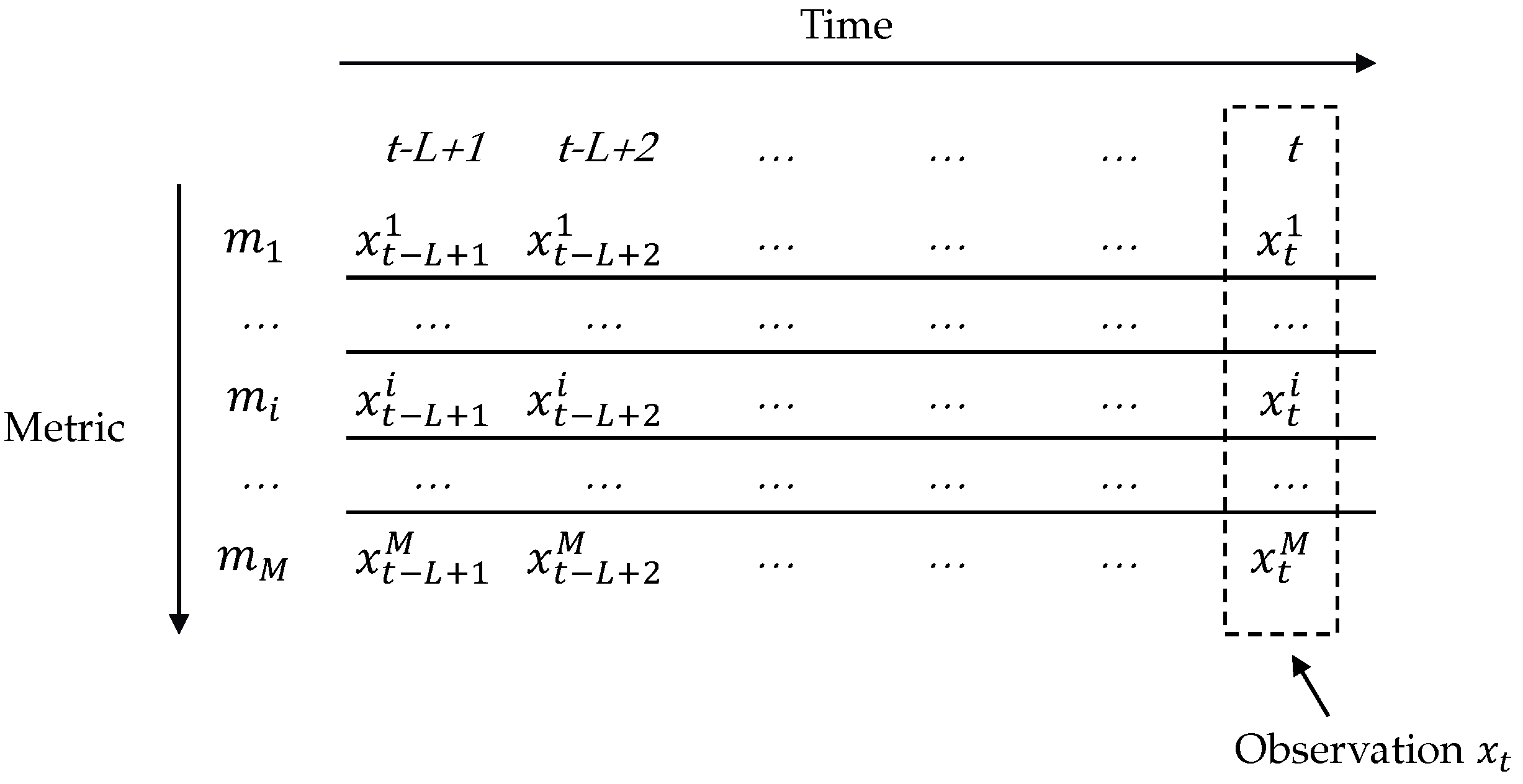
3.1. Multivariate Time Series

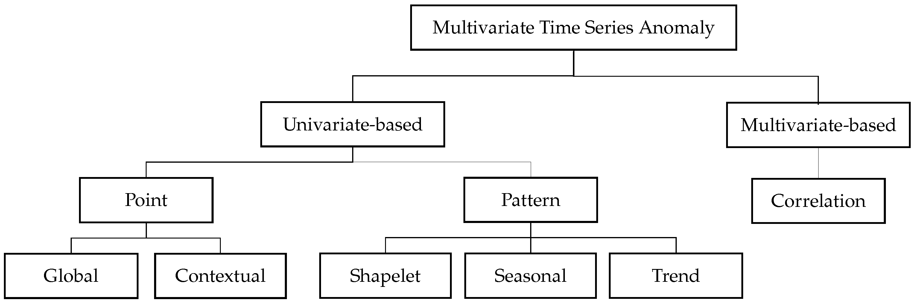
Suppose the monitoring system records successive observations that are equally spaced over time. The observed multivariate time series is denoted by a set of observations $X=\{x_1,...,x_N\}$, $X\in {\mathbb{R}}^{M\times N}$, where M is the number of metrics and N is data length, respectively. Each observation $x_t\in {\mathbb{R}}^M$ is measured at a specific timestamp t. To model the dependency of observations in the temporal dimension, we transform the MTS to a set of window samples to further feed as inputs to the model.

Denote $W=\{w_1,\cdots ,w_{N-L+1}\}$ is a sequence of window samples where L is the window size. A window sample $w_t=\{x_{t-L+1},\cdots ,x_t\}$ at timestamp t is illustrated in Figure 1.

3.2. Anomaly Types

An anomaly is an observation that deviates so much from the other observations as to arouse suspicious [27]. In practice, detecting anomalies is non-trivial because a significant amount of noise may be contained in the data, making the separation between noise and anomaly difficult to define. Therefore, anomalies are often determined according to application-specific criteria and the interest of the analyst. Recently, several studies [10,14,28,29] have attempted to define abnormal behaviors in time series data. Deriving from the previous works, we summarize the anomaly types as univariate-based and multivariate-based, as shown in Figure 2.

In univariate-based anomaly type, abnormal behaviors can be determined by a single time series. According to [26], anomalies are classified into point and pattern-wise behaviors. Point-wise anomalies occur only on individual time points. In that, global anomalies are the points that spike significantly from the rest of the points, while contextual anomalies glitch from their neighboring points. On the other hand, a pattern-wise behavior is caused by a sequence of continuous points. The major causes might be dissimilar shapelets, seasonality changes, and trend alternations. Shapelet anomalies are the sequences with dissimilar basic shapelets compared to the normal shapelet. Despite having similar basic shapelets, seasonal anomalies are caused by unusual seasonalities compared to the overall seasonality. Trend anomalies can be determined by a permanent shift in the mean of the data.

Unlike the univariate-based anomaly type, multivariate-based anomalies occur when the relationships among multiple metrics are violated compared to the historical relationships, as mentioned in [10].

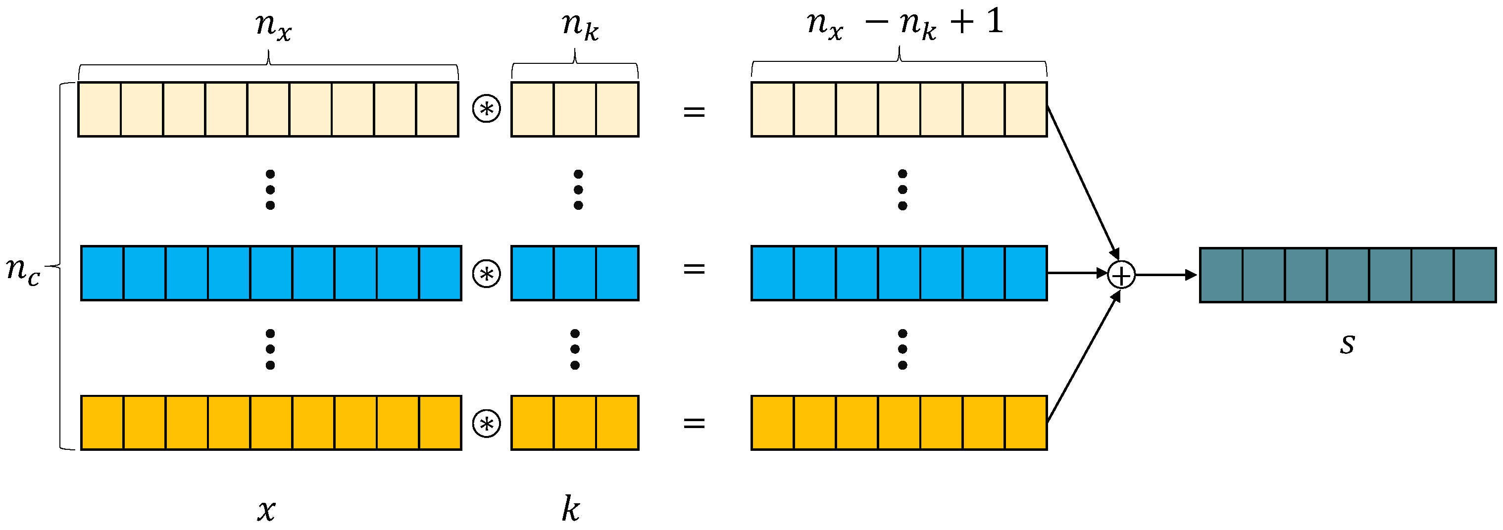
3.3. Convolutional Neural Network

Originally, convolutional neural network was designed for computer vision tasks such as image classification, image segmentation, or face recognition. The data format for these tasks is two-dimensional data, such as images and videos. Therefore, the CNNs processing 2D data are often referred to as 2D CNNs. Due to the need to process 1D (one-dimensional) signals, 1D CNNs, a modified version of 2D CNNs, have been developed [30].

The main component of CNN is convolution kernels, which can extract various features or patterns in the input using convolution operations. The convolution operation uses a convolution kernel, which contains kernel weights to slide over the input sequence and compute a weighted average. The operation convolution with a kernel k on a univariate time series x is defined as:

$$s_t=(x⊛k)\left[t\right]=\sum _{i=1}^{n_k}{x}_{t-i+1}{k}_i$$

(1)

where $s_t$ is the output of time step t, ⊛ is the convolution operator, and $n_k$ is the size of the kernel k. The output result is one-dimensional and its length is $n_x-n_k+1$, where $n_x$ is number of time steps in x. To obtain an output which has the same length as the input, zero padding is applied to the input sequence before performing the operation convolution. As multivariate time series data contains multiple metrics (channels), the kernel k with only one channel will not be meaningful to apply across different channels because of the nature of each metric. Thus, a multi-channel kernel k is created to treat each channel of the input independently. The convolution operation with a multi-channel kernel k on multi-channel data x is:

$$s_t=(x⊛k)\left[t\right]=\sum _{c=1}^{n_c}\sum _{i=1}^{n_k}{x}_{c,t-i+1}{k}_{c,i}$$

(2)

where $n_c$ is number of channels in the data, $x_{c,t-i+1}$ is the measurement of cth channel at time step $t-i+1$. The convolution on the multi-channel data is almost similar as on the single channel, and the difference between these two is an additional summation accross all channels. This summation is the one that implicitly learns the dependency among different metrics in the multi-channel data. Figure 3 illustrates the 1D convolution operation for multivariate time series data.

3.4. Variational Autoencoder

A variational autoencoder is an autoencoder structured as a Bayesian network that learns the relationship between two random variables, latent variable z and observed variable x. The latent variable z is constrained to follow a pre-defined prior distribution $p\left(z\right)$, usually a standard normal distribution. On the other hand, the distribution of the likelihood $p\left(x\right|z)$ can be defined as Normal or Bernoulli, depending on the task. In the Bayesian network, obtaining the posterior distribution of the latent variable $p\left(z\right|x)$ is the main focus. However, the true posterior is intractable for a continuous latent space z [31]. Thus, the variational inference technique is used to approximate the posterior.

As a variational inference algorithm, the SGVB estimator [32] can be used effectively to estimate the true posterior. The algorithm uses a variational net as qnet and a generative net as pnet to maximize the evidence lower bound ELBO for training the VAE model. The ELBO is:

$$\begin{array}{cc}\hfill \mathcal{L}(x,\theta ,\varphi )& ={\mathbb{E}}_{q_{\varphi }\left(z\right|x)}[log{p}_{\theta }\left(x\right|z)]-KL[q_{\varphi }\left(z\right|x)\left|\right|p_{\theta }\left(z\right)]\hfill \\ \hfill & ={\mathbb{E}}_{q_{\varphi }\left(z\right|x)}[log{p}_{\theta }\left(x\right|z)+log{p}_{\theta }\left(z\right)-log{q}_{\varphi }\left(z\right|x)]\hfill \end{array}$$

(3)

where $\theta$ and $\varphi$ are parameters of $pnet$ and $qnet$, respectively. $KL$ is the Kullback-Leibler divergence, this term is to measure the difference between the approximated posterior $q_{\varphi }\left(z\right|x)$ and the prior distribution $p_{\theta }\left(z\right)$. The expectation with $q_{\varphi }$ is approximated by taking L samples using Monte Carlo integration [33] as Equation (4), where $f\left(z^{\left(l\right)}\right)$ are sampled from $q_{\varphi }\left(z\right|x)$.

$${\mathbb{E}}_{q_{\varphi }\left(z\right|x)}\left[f\left(z\right)\right]\approx \frac{1}{L}\sum _{l=1}^{L}f\left(z^{\left(l\right)}\right)$$

(4)

4. Proposed Method

4.1. Proposed Architecture

The overall architecture of the MST-VAE is illustrated in Figure 4. The proposed architecture comprises an encoder as a variational net or $qnet$ and a decoder as a generative net or $pnet$. In this paper, we assume that the multivariate time series are generated from Gaussian processes. Therefore, the prior distribution $p_{\theta }\left(z\right)$ is chosen as a normal standard $\mathcal{N}(0,\mathbf{I})$. The posterior distributions of the latent $q_{\varphi }\left(z\right|x)$ and the observed $p_{\theta }\left(x\right|z)$ are multivariate Gaussians $\mathcal{N}({\mu }_z,{\sigma }_z^2\mathbf{I})$ and $\mathcal{N}({\mu }_x,{\sigma }_x^2\mathbf{I})$, respectively. The ${\mu }_z$, ${\mu }_x$ and ${\sigma }_z^2$, ${\sigma }_x^2$ are means and variances of independent Gaussian components.

Since the model inputs are window samples mentioned in Section 3.1, notation x in the architecture is implicitly referred to as a window sample in the MTS. To obtain the complex temporal patterns, the multi-scale module, which is the main component of the MST-VAE, is first applied to the input. The main idea of the multi-scale module is that different kernel sizes are employed to extract various temporal patterns. The kernel size in the short-scale module is relatively small compared to it in the long-scale module. In the hidden layers, we stack multiple Conv1D layers to reduce the temporal dimension of the input, and a stride of 2 is used in each Conv1D for downsizing. Furthermore, the number of Conv1D layers in the hidden layers is chosen depending on the window size. For anomaly detection in time series, compressing the input to a lower-dimensional representation has two main reasons. First, the low dimensional latent variable can capture the main patterns with a small amount of information from the input. Second, as the training data is commonly supposed to be normal, using a low dimensional latent variable helps the model learn the normal patterns from the data. Then, in the inference phrase, the dimension reduction can throw away information of some abnormal points since the latent variable tries to capture normal patterns from the input, leading the latent z for an abnormal input x, which might be indistinguishable from normal ones [1]. However, the latent variable may fail to capture normal patterns if there are too many anomalies in the input x. After extracting multi-scale features, the outputs of the short and long-scale modules are concatenated along the channel axis. To ensure the number of channels of z is the same as in the input, a convolutional map reduction layer (kernel size = 1) [34] is used to reduce the channel dimensionality. Similar to [10], we choose to derive means ${\mu }_z$ and log standard deviations $log{\sigma }_z$ from Conv1D layers. The log standard deviation is used instead of the standard deviation to ensure the numerical stability in computation. Moreover, we also clip the log standard deviations to avoid unbounded values when standard deviations are extremely close to zero.

In order to reconstruct the input from the latent z, the same process as in the $qnet$ is employed to the $pnet$ except for replacing Conv1D layers in the hidden and feature reduction layers by upsampling layers (Deconv1D).

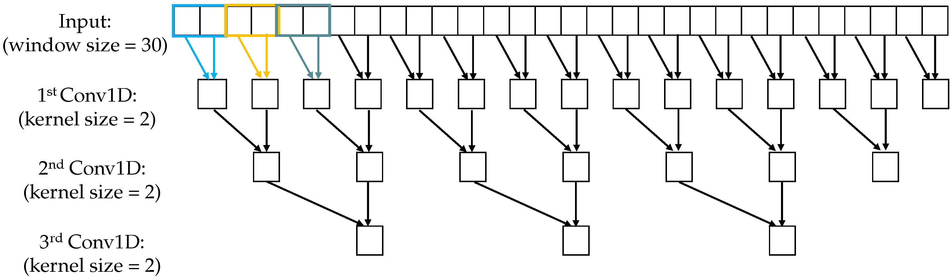
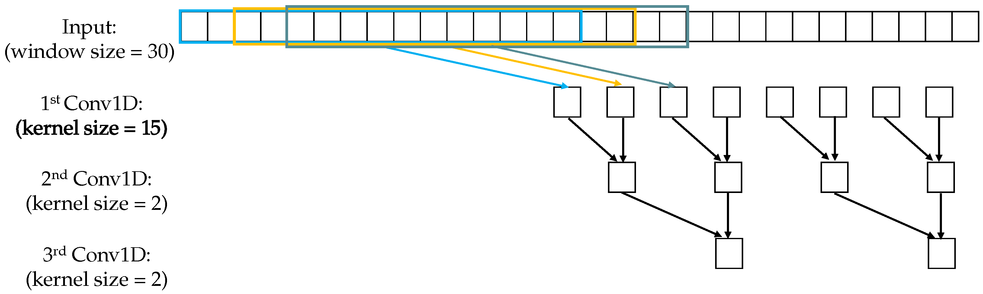
4.2. Multi-Scale Convolutional Kernels

As mentioned in Section 4.1, we use a small kernel size for the short-scale module and a large kernel size for the long-scale module. Kernel sizes 2 and 15 are chosen empirically to apply to the short and long scales, respectively. The reason is that the kernel size of 2 aims to extract short temporal patterns, which are beneficial to detect point anomalies since the duration of point-wise anomalies is short (caused by individual time points). On the other hand, the kernel size of 15 tries to capture longer patterns to trigger pattern anomalies, since the duration of pattern-wise anomalies is long (caused by a sequence of continuous points). Moreover, multi-scale convolutional kernels help the model jointly learn patterns at different scales [34].

While the kernel size of 2 is fixed for the short scale, the kernel size for the long scale can be changed. If the kernel size is too small, it is difficult to capture long patterns. Otherwise, too large kernel size will increase false positives because of overfitting. Note that different kernel sizes are only used for the first Conv1D in the hidden layers; the kernel size of 2 is fixed from the next layer. Figure 5 and Figure 6 illustrates the feature extraction using different temporal scales.

4.3. Model Training and Inference

Before training the model, we preprocess the raw data by filling missing values with zeros and normalizing data using MinMaxScaler. Then, we transform all observations into window samples, as the model inputs using sliding window. Depending on the monitoring strategies of target systems, MTS data can be either regular or irregular. In the irregular MTS, the data may have various sampling durations or time intervals; thus, it may degrade the performance of anomaly detection methods [35]. However, in the scope of our work, we assume that the data has the same time intervals and lengths among metrics.

In practice, the generated data may not strictly follow Gaussian distributions, which leads to the difficulty of optimizing the reconstruction error ${\mathbb{E}}_{q_{\varphi }\left(z\right|x)}[log{p}_{\theta }\left(x\right|z)]$ in the ELBO. As a result, the model tends to optimize the Kullback-Leibler divergence. That may cause posterior collapse, in which the posterior of the latent variable is equal to its prior. To solve the problem, we adopted $\beta -$VAE [36] to put more weight on the first term of the ELBO while optimizing. We set $\beta =0.2$ as in [37] and observe that this value works well in our experiment. The modified ELBO is defined as:

$$\mathcal{L}(x,\theta ,\varphi )={\mathbb{E}}_{q_{\varphi }\left(z\right|x)}[log{p}_{\theta }\left(x\right|z)]-\beta KL[q_{\varphi }\left(z\right|x)\left|\right|p_{\theta }\left(z\right)]$$

(5)

If we sample directly from the stochastic variable $z\sim \mathcal{N}({\mu }_z,{\sigma }_z^2\mathbf{I})$, computing the ELBO when training VAE will be infeasible because the process of sampling is not differentiable. Thus, the stochastic gradient descent cannot be applied to the model. To solve this problem, SGVB proposed the re-parameterization trick, which creates a random variable $ϵ\sim \mathcal{N}(0,\mathbf{I})$ for sampling independently with z, such that z can be rewritten as $z\left(ϵ\right)={\mu }_z+{\sigma }_zϵ$. As recommended in SGVB, sampling one sample is sufficient for computing the ELBO in the training model; thus, we also set L = 1.

In the inference phase, we calculate the reconstruction probability as the anomaly score, which can be referred to in [1,10]. To classify the observation at timestep t into normal or abnormal, the window sample $w_t=\{x_{t-L+1},\cdots ,x_t\}$ is used to infer from the trained model. Although the model output has all the scores corresponding to each observation in the window sample $w_t$, we only use the score of the last observation $x_t$ for anomaly detection. During detection, a window sample may contain abnormal points, and these points may cause a bias to the embedded representation z, then affect the reconstruction probability. To reduce the effect of anomalies in the input, we adopted MCMC imputation [10,38] to replace anomalous points with normal points. Based on the imputation, a more reasonable embedded representation could be achieved, thus helping the model to detect anomalies more accurately. The procedure for MCMC imputation is described as follows: given an input x; the embedded representation z is sampled from $q_{\varphi }\left(z\right|x)$; then, a reconstruction is obtained from $pnet$. The last observation in x is replaced by the last observation in the reconstruction to achieve a new input $\tilde{x}$. We iterate this procedure M times to reduce the bias and achieve a better representation. Note that the output of current iteration will be the input of the next iteration. After finishing the MCMC imputation, the reconstruction probability can be calculated using a Monte Carlo integration, which is similar to Equation (4). The anomaly score is:

$$scor{e}_{anomaly}=-{\mathbb{E}}_{q_{\varphi }\left(z\right|x)}[log{p}_{\theta }\left(x\right|z)]=-\frac{1}{L}\sum _{l=1}^L[log{p}_{\theta }\left(x\right|z^{\left(l\right)})]$$

(6)

where $z^{\left(l\right)}$ is sampled from $q_{\varphi }\left(z\right|\tilde{x})$. An observation with an anomaly score higher than the predefined threshold will be classified as an anomaly.

5. Experiment

5.1. Datasets

To evaluate the performance of the proposed method, we conducted the experiment on five real-world datasets: ASD (Application Server Dataset), SMD (Server Machine Dataset), PSM(Pooled Server Metrics) from Ebay, SWaT (Secure Water Treatment), and WADI (Water Distribution). The first three datasets are all collected from large Internet companies. These datasets contain system metrics (CPU, network, memory, etc.) characterizing the statuses of different machines. SWaT and WADI are datasets about water treatment plant and the data are generated from testbeds. While SWaT and WADI have no anomalies in training data, a small amount of abnormal points might be contained in the three server datasets.

Table 1. Details of datasets.

Dataset	No. Entities	No. Metrics	Train	Test	Anomaly Rate
ASD	12	19	102,331	51,840	4.61
SMD	12	38	304,168	304,174	5.84
PSM	N/A	25	132,841	87,841	11.07
SWaT	1	51	475,200	449,919	12.13
WADI	1	118	789,371	172,801	5.85

presents more detailed information about five datasets such as the number of entities, number of metrics or channels, number of points in train and test sets, and anomaly rate.

Since ASD and SMD contain 12 entities in each dataset, the evaluation results of MST-VAE on these datasets will be the average of all 12 entities.

5.2. Experiment Setup

The experiments are executed in a PC with Windows 10, Intel(R) Core(TM) i7-10700 (16 CPUs), NVIDIA RTX 2060, and 16 GB of RAM. The environment is set up with Anaconda 4.11.0, Python 3.6.13, and Tensorflow 1.12.0. Deriving from the study [10],

Table 2. Hyperparameters values used in experiments.

Hyperparameter	Value
Window length	100 for ASD, SMD; 30 for PSM, SWaT, and WADI
No. Conv1D layers in hidden layers	3 for window length = 100, 2 for window length = 30
Activation function	ReLU is applied for Conv1D in hidden layers
L2 regularization	1 × 10${}^{-4}$
Clip values for log std	min = −5, max = 2
Batch size	100
Train validaion split	7:3 for ASD, SMD; 9:1 for PSM, SWaT, and WADI
Number of z samples for Monte Carlo integration	100
No. MCMC iterations	10

lists all hyperparameters used in the experiments. Our code is released at https://github.com/tuananhphamds/MST-VAE (accessed on 26 July 2022).

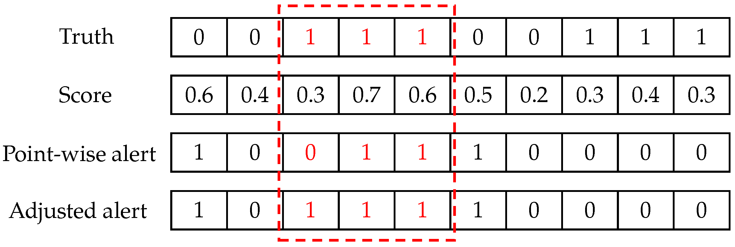
5.3. Evaluation Metrics

We use best F1 Score denoted as $F{1}_{best}$ to compare detection performance between MST-VAE and baseline methods. Unlike conventional F1 Score which is calculated by a threshold selection method, $F{1}_{best}$ can estimate the best possible performance of a model. To obtain $F{1}_{best}$, we enumerate all possible F1s from all anomaly scores from the test data, then search for the highest F1.

When an anomaly event occurs, it often happens with continuous observations and forms an anomaly segment. Thus, it is acceptable for a model to trigger an alert for any observation within the anomaly segment. Therefore, we adopted the point-adjust approach [1] used widely in MTS anomaly detection studies. If any point in an anomaly segment is detected correctly, we say that this segment is totally detected. This means all points in the segment are treated as if they are detected correctly. Figure 7 illustrates how to detect anomalies using the adjusted-F1. The red box covers an anomaly segment including three observations. For the point-wise detector, there are only two alerts, which are triggered in the third row. Applying the adjust-point method, the first point in the anomaly segment is modified and treated as being detected correctly in the fourth row.

Equation (7) presents how to calculate adjusted-F1.

$$\begin{array}{c}F{1}_{adjusted}=\frac{2 \times Precision \times Recall}{Precision + Recall}\\ \\ Precision=\frac{T{P}_{adjusted}}{T{P}_{adjusted} + FP}\\ \\ Recall=\frac{T{P}_{adjusted}}{T{P}_{adjusted} + FN}\end{array}$$

(7)

5.4. Performance Evaluation

5.4.1. Anomaly Detection Results

We compared the detection performance of MST-VAE with ten baseline methods on the five real-world datasets. Because the randomness in the training process may affect the detection results, we executed five repeated experiments for each method and obtain the highest score. The performance of different methods are presented in

Table 3. Performance comparison of the best F1 Scores of different baseline methods on five datasets.

Baselines	ASD	SMD	PSM	SWaT	WADI	Average
LOF	0.7954	0.8954	0.7609	0.8167	0.4689	0.7475
DAGMM	0.7436	0.9528	0.9399	0.7997	0.4306	0.7733
Isolation Forest	0.7115	0.9516	0.9200	0.8413	0.6674	0.8184
LSTM-NDT	0.4061	0.7687	0.8319	0.8133	0.5067	0.6653
MAD-GAN	0.6325	0.8966	0.6158	0.8431	0.7085	0.7393
LSTM-VAE	0.5964	0.9501	0.7951	0.8223	0.5452	0.7418
USAD	0.7987	0.9024	0.7606	0.8227	0.4275	0.7424
OmniAnomaly	0.8344	0.9628	0.9076	0.7344	0.7927	0.8464
MSCRED	0.5948	0.8252	0.7468	0.8346	0.5469	0.7097
InterFusion	0.9531	0.9817	0.9511	0.9280	0.9103	0.9448
MST-VAE	0.9766	0.9849	0.9555	0.9407	0.9479	0.9611

. It can be observed that most of the methods achieved the highest performance on the SMD because this dataset mainly contains severe anomalies. Among eleven methods, LSTM-NDT shows the lowest performance due to the difficulty of capturing external factors of prediction-based methods, as discussed in Section 1. Without considering the temporal information in the time series data, the classical unsupervised methods fail to detect context and pattern anomalies and their performance results degrade in ASD. Among the five datasets, only the WADI dataset has the range values of normal data shifted in the test set. These range values are unseen in the training data, causing the performance of most methods to drop dramatically (0.4275 in USAD). However, the results demonstrate that MST-VAE (0.9479) and Interfusion (0.9103) can still adapt to unseen data.

Interfusion is the first study that explores both temporal dependency and dependency across multiple metrics, which helps the detection results stable among different datasets. Moreover, MST-VAE implicitly learns dependency between metrics using Conv1Ds and extracts complex temporal information based on the multi-scale module. For that reason, MST-VAE has demonstrated an improvement in detection performance compared to Interfusion, of 1.63% on average.

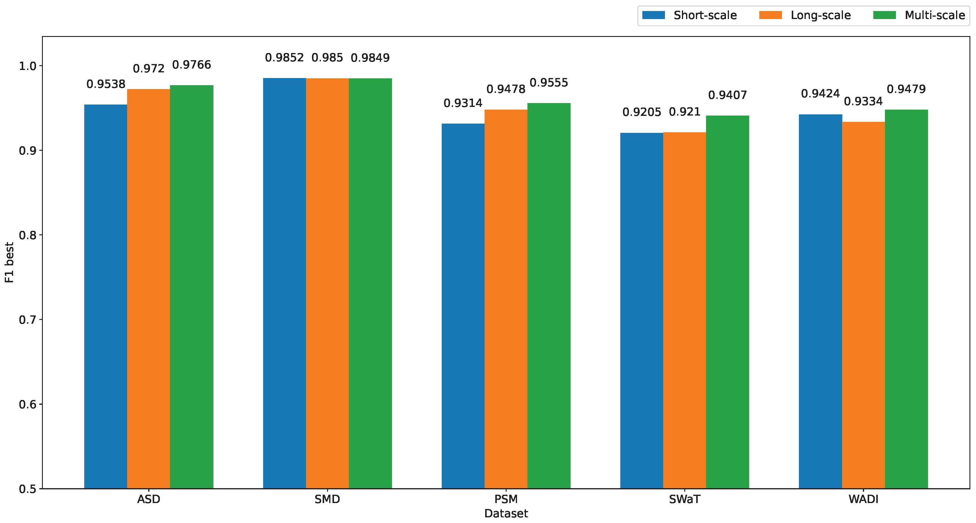
5.4.2. Effect of Multi-Scale Kernels on the Model Performance

To verify the effectiveness of the multi-scale module, we evaluate the performance of MST-VAE with short-scale only, long-scale only, and finally combine both as a multi-scale. The performance comparison between three modules are shown in Figure 8. To evaluate the model using a single scale, we removed the concatenate and feature reduction layers in the MST-VAE architecture. The overall results demonstrate that combining different kernel scales can enhance the anomaly detection performance. Since the long-scale kernel is able to extract longer temporal information, it helps the model to detect mild anomalies. Specifically, the long-scale module shows higher performance compared to the short-scale module in ASD and PSM datasets. In the datasets SMD and SWAT, there is not much difference between the short-scale and long-scale modules because anomalies in these datasets are easier to be detected (large spikes on several metrics).

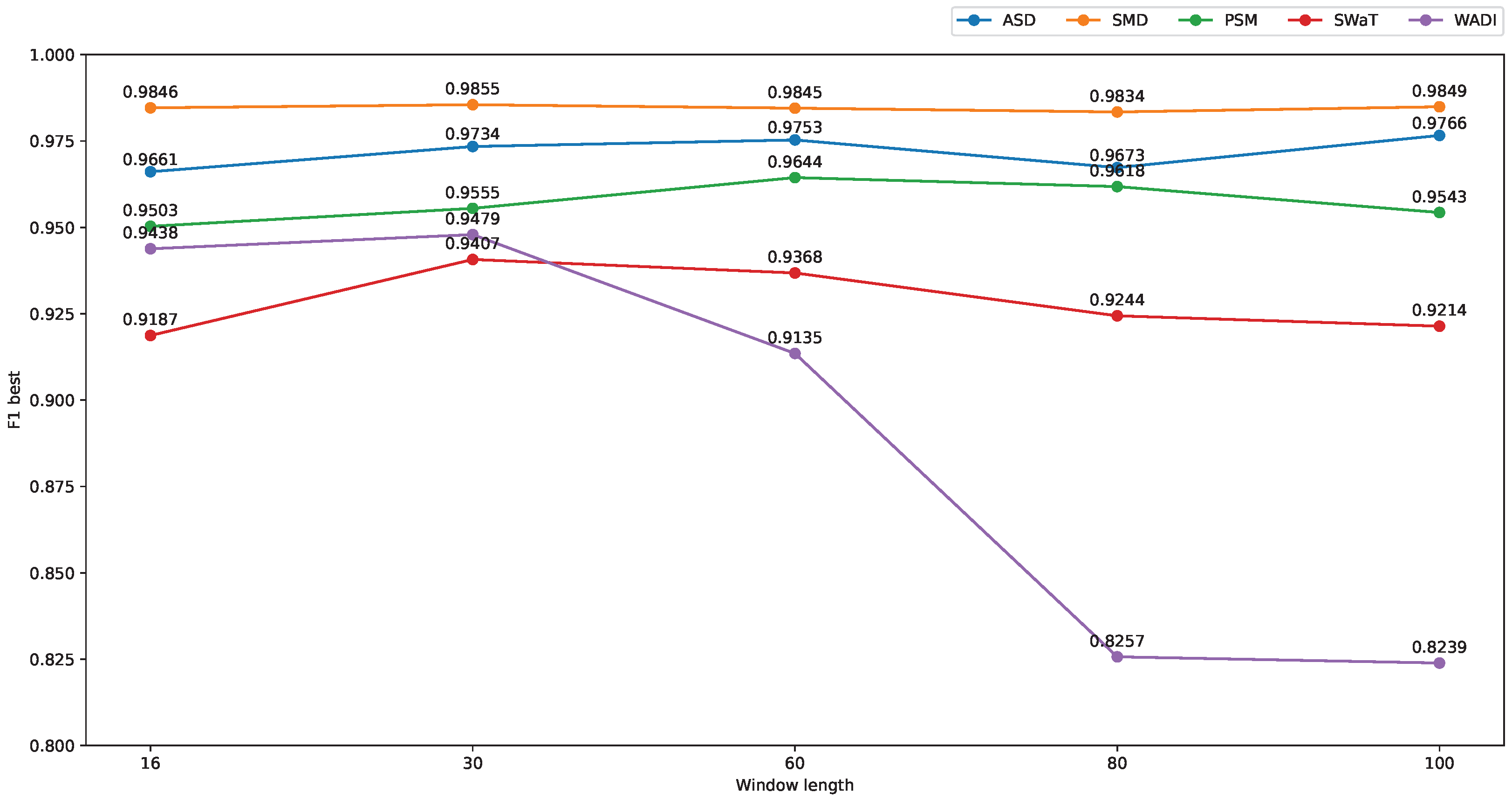
5.4.3. Effect of Window Lengths on the Model Performance

We evaluated the model performance with various window lengths on the five datasets, and the effect of window lengths on the model performance is shown in Figure 9. For window lengths 16 and 30, we applied two Conv1D hidden layers, while three layers were employed for the rest of the window lengths. It can be observed that there is not much difference in detection performance for different window lengths in the SMD and PSM. The reason is that most anomalies in SMD and PSM are large spikes, because it does not need a large window length for detection. Otherwise, mild and context anomalies are contained in the ASD, and the longer window length might help to trigger these types of anomalies. Specifically, MST-VAE achieved 0.9661 with window length 16 and 0.9766 with window length 100. However, for the water treatment datasets SWaT and WADI, MST-VAE works well with the window length of 30, and its performance tends to degrade when the window length increases.

5.4.4. Training Time

MST-VAE not only improved the detection performance but also achieved less training time compared to the InterFusion method. Since MST-VAE does not use GRU layers in its architecture, the model can benefit from parallel computation and accelerate the training process.

Table 4. Training time (second) per epoch on each dataset.

Baselines	ASD	SMD	PSM	SWaT	WADI
InterFusion	15.38	49.39	111.92	499.2	611.07
MST-VAE	1.76	7.12	10	92.93	151.2
Acceleration factor	8.74	6.94	11.19	5.37	4.04

compares training time per epoch on the five datasets between MST-VAE and Interfusion. The results demonstrate that MST-VAE can reduce training time by an average of 7.25 times.

6. Conclusions

Inspired by the state-of-the-art InterFusion, we proposed an effective and practical architecture for anomaly detection in multivariate time series data. While the short-scale module can extract short temporal patterns, which is beneficial for detecting severe anomalies (large spikes), the long-scale module tends to embed longer temporal information to trigger context and pattern anomalies. From that observation, we improved the temporal embedding by proposing multi-scale convolution kernels in the Variational Autoencoder.

The performance comparison with ten baseline methods demonstrates that MST-VAE outperforms the classical unsupervised, prediction-based, and reconstruction-based methods. Compared to InterFusion, MST-VAE also demonstrates an improvement in detection performance and training speed.

The MTS data in this study is assumed to be generated from Gaussian processes. Therefore, the model might not work well with intricate data. In future work, we plan to explore multivariate time series with different distributions to make the model widely adaptive.

References

1. Xu, H.; Chen, W.; Zhao, N.; Li, Z.; Bu, J.; Li, Z.; Liu, Y.; Zhao, Y.; Pei, D.; Feng, Y.; et al. Unsupervised Anomaly Detection via Variational Auto-Encoder for Seasonal KPIs in Web Applications. In Proceedings of the 2018 World Wide Web Conference on World Wide Web, Lyon, France, 23–27 April 2018; pp. 187–196. [Google Scholar]
2. Su, Y.; Zhao, Y.; Niu, C.; Liu, R.; Sun, W.; Pei, D. Robust Anomaly Detection for Multivariate Time Series through Stochastic Recurrent Neural Network. In Proceedings of the 25th ACM SIGKDD International Conference on Knowledge Discovery and Data Mining, Anchorage, AK, USA, 4–8 August 2019; pp. 2828–2837. [Google Scholar]
3. Zhang, C.; Song, D.; Chen, Y.; Feng, X.; Lumezanu, C.; Cheng, W.; Ni, J.; Zong, B.; Chen, H.; Chawla, N.V. A Deep Neural Network for Unsupervised Anomaly Detection and Diagnosis in Multivariate Time Series Data. In Proceedings of the AAAI Conference on Artificial Intelligence, Honolulu, HI, USA, 27 January–1 February 2019; pp. 1409–1416. [Google Scholar]
4. Sánchez-Fernández, A.; Baldán, F.J.; Sainz-Palmero, G.I.; Benítez, J.M.; Fuente, M.J. Fault detection based on time series modeling and multivariate statistical process control. Chemom. Intell. Lab. Syst. 2018, 182, 57–69. [Google Scholar] [CrossRef]
5. Hundman, K.; Constantinou, V.; Laporte, C.; Colwell, I.; Soderstrom, T. Detecting Spacecraft Anomalies Using LSTMs and Nonparametric Dynamic Thresholding. In Proceedings of the 24th ACM SIGKDD International Conference on Knowledge Discovery & Data Mining, London, UK, 19–23 August 2018; pp. 387–395. [Google Scholar]
6. Blázquez-Gacía, A.; Conde, A.; Mori, U.; Lozano, J.A. A Review on Outlier/Anomaly Detection in Time Series Data. ACM Comput. Surv. 2022, 54, 1–33. [Google Scholar] [CrossRef]
7. Garg, A.; Zhang, W.; Samaran, J.; Savitha, R.; Foo, C.S. An Evaluation of Anomaly Detection and Diagnosis in Multivariate Time Series. IEEE Trans. Neural Netw. Learn. Syst. 2022, 33, 2508–2517. [Google Scholar] [CrossRef] [PubMed]
8. Zhou, Y.; Qin, R.; Xu, H.; Sadiq, S.; Yu, Y. A Data Quality Control Method for Seafloor Observatories: The Application of Observed Time Series Data in the East China Sea. Sensors 2018, 18, 2628. [Google Scholar] [CrossRef] [Green Version]
9. Carrera, D.; Rossi, B.; Fragneto, P.; Boracchi, G. Online anomaly detection for long-term ECG monitoring using wearable devices. Pattern Recognit. 2019, 88, 482–492. [Google Scholar] [CrossRef]
10. Li, Z.; Zhao, Y.; Han, J.; Su, Y.; Jiao, R.; Wen, X.; Pei, D. Multivariate Time Series Anomaly Detection and Interpretation using Hierarchical Inter-Metric and Temporal Embedding. In Proceedings of the 27th ACM SIGKDD Conference on Knowledge Discovery & Data Mining, Washington, DC, USA, 14–18 August 2021; pp. 3220–3230. [Google Scholar]
11. Audibert, J.; Michiardi, P.; Guyard, F.; Marti, S.; Zuluaga, M.A. USAD: UnSupervised Anomaly Detection on Multivariate Time Series. In Proceedings of the 26th ACM SIGKDD International Conference on Knowledge Discovery Data Mining, New York, NY, USA, 6–10 July 2020; pp. 3395–3404. [Google Scholar]
12. Zhao, Y.; Zhang, X.; Shang, Z.; Cao, Z. A Novel Hybrid Method for KPI Anomaly Detection Based on VAE and SVDD. Symmetry 2021, 13, 2104. [Google Scholar] [CrossRef]
13. Braei, M.; Wagner, S. Anomaly Detection in Univariate Time-Series: A Survey on the State-of-the-Art. arXiv 2020, arXiv:2004.00433. [Google Scholar]
14. Choi, K.; Yi, J.; Park, C.; Yoon, S. Deep Learning for Anomaly Detection in Time-Series Data: Review, Analysis, and Guidelines. IEEE Access 2021, 9, 120043–120065. [Google Scholar] [CrossRef]
15. Pan, D.; Song, Z.; Nie, L.; Wang, B. Satellite Telemetry Data Anomaly Detection Using Bi-LSTM Prediction Based Model. In Proceedings of the 2020 IEEE International Instrumentation and Measurement Technology Conference (I2MTC), Dubrovnik, Croatia, 25–28 May 2020; pp. 1–6. [Google Scholar]
16. Malhotra, P.; Ramakrishnan, A.; Anand, G.; Vig, L.; Agarwal, P.; Shroff, G. LSTM-based encoder-decoder for multi-sensor anomaly detection. arXiv 2016, arXiv:1607.00148. [Google Scholar]
17. Nguyen, H.D.; Tran, K.P.; Thomassey, S.; Hamad, M. Forecasting and Anomaly Detection approaches using LSTM and LSTM Autoencoder techniques with the applications in supply chain management. Int. J. Inf. Manag. 2020, 57, 102282. [Google Scholar] [CrossRef]
18. Thill, M.; Konen, W.; Wang, H.; Bäck, T. Temporal convolutional autoencoder for unsupervised anomaly detection in time series. Appl. Soft Comput. 2021, 112, 107751. [Google Scholar] [CrossRef]
19. An, J.; Cho, S. Variational Autoencoder Based Anomaly Detection Using Reconstruction Probability; Technical Report; SNU Data Mining Center: Seoul, Korea, 2015. [Google Scholar]
20. Li, L.; Yan, J.; Wang, H.; Jin, Y. Anomaly Detection of Time Series With Smoothness-Inducing Sequential Variational Auto-Encoder. IEEE Trans. Neural Netw. Learn. Syst. 2020, 32, 1177–1191. [Google Scholar] [CrossRef] [PubMed]
21. Gao, J.; Song, X.; Wen, Q.; Wang, P.; Sun, L.; Xu, H. Robusttad: Robust time series anomaly detection via decomposition and convolutional neural networks. arXiv 2020, arXiv:2002.09535. [Google Scholar]
22. Breunig, M.M.; Kriegel, H.P.; Ng, R.T.; Sander, J. LOF: Identifying Density-Based Local Outliers. In Proceedings of the 2000 ACM SIGMOD International Conference on Management of Data, Dallas, TX, USA, 15–18 May 2000; pp. 93–104. [Google Scholar]
23. Zong, B.; Song, Q.; Min, M.R.; Cheng, W.; Lumezanu, C.; Cho, D.; Chen, H. Deep autoencoding gaussian mixture model for unsupervised anomaly detection. In Proceedings of the 6th International Conference on Learning Representations, Vancouver, BC, Canada, 30 April–3 May 2018. [Google Scholar]
24. Liu, F.T.; Ting, K.M.; Zhou, Z.H. Isolation forest. In Proceedings of the 8th IEEE International Conference on Data Mining, Pisa, Italy, 15–19 December 2008; pp. 413–422. [Google Scholar]
25. Li, D.; Chen, D.; Goh, J.; Ng, S.-K. MAD-GAN: Multivariate Anomaly Detection for Time Series Data with Generative Adversarial Networks. In Proceedings of the 28th International Conference on Artificial Neural Networks, Munich, Germany, 17–19 September 2019; pp. 703–716. [Google Scholar]
26. Park, D.; Hoshi, Y.; Kemp, C.C. A multimodal anomaly detector for robot-assisted feeding using an lstm-based variational autoencoder. IEEE Robot. Autom. Lett. 2018, 3, 1544–1551. [Google Scholar] [CrossRef] [Green Version]
27. Aggarwal, C.C. An introduction to outlier analysis. In Outlier Analysis; Springer: Berlin/Heidelberg, Germany, 2017; pp. 1–34. [Google Scholar]
28. Lai, K.H.; Zha, D.; Xu, J.; Zhao, Y.; Wang, G.; Hu, X. Revisiting Time Series Outlier Detection: Definitions and Benchmarks. In Proceedings of the Thirtyfifth Conference on Neural Information Processing Systems Datasets and Benchmarks Track (Round 1), Online, 7–10 December 2021. [Google Scholar]
29. Xu, J.; Wu, H.; Wang, J.; Long, M. Anomaly Transformer: Time series anomaly detection with association discrepancy. In Proceedings of the Tenth International Conference on Learning Representations, Online, 25–29 April 2022. [Google Scholar]
30. Kiranyaz, S.; Avci, O.; Abdeljaber, O.; Ince, T.; Gabbouj, M.; Inman, D.J. 1D convolutional neural networks and applications: A survey. arXiv 2019, arXiv:1905.03554. [Google Scholar] [CrossRef]
31. Blei, D.M.; Kucukelbir, A.; McAuliffe, J.D. Variational inference: A review for statisticians. J. Am. Stat. Assoc. 2017, 112, 859–877. [Google Scholar] [CrossRef] [Green Version]
32. Kingma, D.P.; Welling, M. Auto-encoding variational bayes. In Proceedings of the 2nd International Conference on Learning Representations, Banff, AB, Canada, 14–16 April 2014. [Google Scholar]
33. Geweke, J. Bayesian Inference in Econometric Models Using Monte Carlo Integration. Econometrica 1989, 57, 1317–1339. [Google Scholar] [CrossRef]
34. Szegedy, C.; Liu, W.; Jia, Y.; Sermanet, P.; Reed, S.; Anguelov, D.; Erhan, D.; Vanhoucke, V.; Rabinovich, A. Going deeper with convolutions. In Proceedings of the 2015 Computer Vision and Pattern Recognition IEEE, Boston, MA, USA, 7–12 June 2015; pp. 1–9. [Google Scholar]
35. He, S.; Li, Z.; Wang, J.; Xiong, N.N. Intelligent Detection for Key Performance Indicators in Industrial-Based Cyber-Physical Systems. IEEE Trans. Ind. Inform. 2021, 17, 5799–5809. [Google Scholar] [CrossRef]
36. Higgins, I.; Matthey, L.; Pal, A.; Burgess, C.; Glorot, X.; Botvinick, M.; Mohamed, S.; Lerchner, A. beta-vae: Learning Basic Visual Concepts with a Constrained Variational Framework. In Proceedings of the 5th International Conference on Learning Representations (ICLR 2017), Toulon, France, 24–26 April 2017. [Google Scholar]
37. Wang, Y.; Blei, D.M.; Cunningham, J.P. Posterior collapse and latent variable non-identifiability. In Proceedings of the Neural Information Processing Systems 34 (NeurIPS 2021), Online, 6–14 December 2021. [Google Scholar]
38. Rezende, D.J.; Mohamed, S.; Wierstra, D. Stochastic Backpropagation and Approximate Inference in Deep Generative Models. In Proceedings of the 31st International Conference on Machine Learning (ICML), Beijing, China, 21–26 June 2014; pp. 1278–1286. [Google Scholar]
39. Abdulaal, A.; Liu, Z.; Lancewicki, T. Practical Approach to Asynchronous Multivariate Time Series Anomaly Detection and Localization. In Proceedings of the 27th ACM SIGKDD Conference on Knowledge Discovery and Data Mining (KDD’21), New York, NY, USA, 14–18 August 2021; pp. 2485–2494.
Figure 1. Window sample w t R M × L .
Applsci 12 10078 g001
Figure 2. Anomaly types in multivariate time series.
Applsci 12 10078 g002
Figure 3. 1D convolution operation with a multi-channel kernel on multi-channel data.
Applsci 12 10078 g003
Figure 4. Overall architecture of MST-VAE. Circles are stochastic variables, black rectangles are layers, and red dashed rectangles are multi-scale modules.
Applsci 12 10078 g004
Figure 5. Short-scale module, window size = 30, strides = 2, kernel size = 2, no zero padding.
Applsci 12 10078 g005
Figure 6. Long-scale module, window size = 30, strides = 2, kernel size = 15 (first layer), no zero padding.
Applsci 12 10078 g006
Figure 7. Illustration of adjusted F1 with a threshold of 0.5.
Applsci 12 10078 g007
Figure 8. Performance comparison between short-scale, long-scale, and multi-scale modules.
Applsci 12 10078 g008
Figure 9. Model performance on different window lengths.
Applsci 12 10078 g009