Article

Bayesian Hierarchical Modelling for Uncertainty Quantification in Operational Thermal Resistance of LED Systems

1
Joanneum Research Forschungsgesellschaft mbH, Leonhardstraße 59, 8010 Graz, Austria
2
Materials Center Leoben Forschung GmbH, Roseggerstraße 12, 8700 Leoben, Austria
*
Author to whom correspondence should be addressed.
Appl. Sci. 2022, 12(19), 10063; https://doi.org/10.3390/app121910063
Submission received: 19 August 2022 / Revised: 16 September 2022 / Accepted: 19 September 2022 / Published: 6 October 2022

Abstract

:
Remaining useful life (RUL) prediction is central to prognostics and reliability assessment of light-emitting diode (LED) systems. Their unknown long-term service life remaining when subject to specific operating conditions is affected by various sources of uncertainty stemming from production of individual system components, application of the whole system, measurement and operation. To enhance the reliability of model-based predictions, it is essential to account for all of these uncertainties in a systematic manner. This paper proposes a Bayesian hierarchical modelling framework for inverse uncertainty quantification (UQ) in LED operation under thermal loading. The main focus is on the LED systems’ operational thermal resistances, which are subject to system and application variability. Posterior inference is based on a Markov chain Monte Carlo (MCMC) sampling scheme using the Metropolis–Hastings (MH) algorithm. Performance of the method is investigated for simulated data, which allow to focus on different UQ aspects in applications. Findings from an application scenario in which the impact of disregarded uncertainty on RUL prediction is discussed highlight the need for a comprehensive UQ to allow for reliable predictions.

1. Introduction

The reliability of light-emitting diode (LED) systems is dependent upon numerous factors, including operating temperature, switching pattern, the thermal management system and the LED device itself. The electrical, thermal and optical parameters have a strong mutual dependence defining LED operation. Knowledge about the parameters is key to determine the reliability and the useful operating life of LED systems. One of the essential parameters is the temperature of the LED system under service, which is directly proportional to the total junction-to-ambient thermal resistance of the heat-flow path of the LED application. Guaranteeing low thermal resistance between junction and ambient air is therefore a key requirement for the design and operation of any LED system.
An LED system has many components, such as the LED package, the printed circuit board (PCB), driver optics, the thermal interface material (TIM) and the heat-sink (HS) [1] (see Figure 1). The failure of any component can cause the whole system to fail, and overviews can be found in the literature [2,3,4]. They distinguish between catastrophic, i.e., an abrupt and permanent disruption of a device, and degradation failure modes, i.e., systematic failure over the whole LED system. LED system life-testing must consider both failure types and consider the lesser one to rate LED system life. A common choice for life-testing is power cycling (PC) and increased temperature conditions to emulate the operational conditions of an LED system [5,6,7]. The first acceleration factor is the dwell-time, the duration the system is operating at its maximum steady-state temperature, since the rate of lumen depreciation is strongly correlated to the LED chip temperature, i.e., depreciation increases as the LED junction temperature increases [8]. The second acceleration factor is the temperature change during the on-/off-cycle. Power cycling can lead to thermal fatigue of interconnection technologies such as wire-bonds [5] and solder joints [9]. Solder joint fatigue leads to embrittlement, which in turn increases the thermal resistance. If the thermal resistance, and thus the temperature of the LED system, exceeds a certain threshold, the LED cannot serve its original purpose and needs to be replaced [10].
These acceleration factors are used to build corresponding lifetime models for LEDs. The accuracy of such lifetime prediction models describing the relationship between testing condition and resulting service life crucially depends on various sources of uncertainty. Examples include production uncertainty in device parameters, e.g., the porosity of the die attach or solder interfaces; uncertainty resulting from application, such as mounting on a heat sink via thermal interface materials; measurement noise; uncertainty in initial conditions (e.g., in input parameters of lifetime models); operating uncertainty in the experimental conditions, affecting the accuracy of the equipment used for testing or measuring; or statistical estimation uncertainty.
The literature categorizes uncertainty in three dimensions, cf., e.g., [11,12]: the location of uncertainty, which refers to different sources of uncertainty underlying the system in focus (e.g., production, application, measurement or operation); its levels, ranging from complete knowledge to total ignorance; and last, its nature, i.e., the differentiation between two different types of uncertainty, namely aleatory variability and epistemic uncertainty. Aleatory variability refers to the (natural) intrinsic randomness in any process or model parameter, and epistemic uncertainty results from lack of knowledge or ignorance. Epistemic uncertainty includes parametric and model uncertainty due to imperfect knowledge about parameters and the process of interest. With increased knowledge in the form of more data or the use of more refined models, epistemic uncertainty is reducible in practice, whereas the stochastic component is not; cf. [13,14].
In general, uncertainty quantification (UQ) refers to the process of identifying, characterizing, representing and quantifying all sources of uncertainty within an application to enhance the reliability of model-based predictions and to allow for decision-making at a known level of confidence [15,16]. This is also a key issue in prognostics and health management (PHM), especially in prognostics [17,18]. Since prognostics deals with the prediction of the future evolution of the system’s health, there are several sources of potential uncertainty (e.g., inputs, states, parameters and mathematical models) that might affect these predictions. Therefore, it is essential to address these sources separately and to quantify how they influence the system in focus by capturing the overall uncertainty in the predictions.
Using a probabilistic framework, the whole data-generating process is expressed in terms of probability distributions. The basic concept of probabilistic, or, synonymously, Bayesian inference is to update prior knowledge about unobserved quantities via the likelihood distribution into the posterior distribution. The posterior distribution then reflects the updated knowledge after having observed the data and provides a natural framework for UQ. This allows quantification of the reliability of model predictions by means of credible regions and posterior predictive distributions; cf. [19,20,21]. Bayesian hierarchical models (BHMs) provide a powerful and flexible probabilistic framework for quantification and analysis of multiple sources of uncertainty [22,23,24,25]. The particular modelling of prior information in terms of several conditional prior distributions allows to account for different types of uncertainty in input parameters at different levels of the hierarchy and to differentiate between aleatory and epistemic uncertainty therein [21].
In this paper, a BHM framework is proposed to quantify the overall uncertainty in the initial LED temperature change caused by thermal stress. Its variability rests upon various sources, such as measurement and operating uncertainty and the LED’s operational thermal resistance, which is subject to system and application variability. The BHM is built upon an inverse problem formulation of a physically derived model used to describe the initial temperature change. Posterior inference for this BHM is based on Markov chain Monte Carlo (MCMC) methods using a Metropolis–Hastings (MH) algorithm.
Since temperature change, and particularly the initial temperature change, is a crucial factor for LED degradation due to thermal fatigue, its reliable quantification is decisive for the stability of lifetime predictions. Thus, accounting for different potential types and sources of uncertainty in the initial state is an important aspect in PC and the novelty of our approach. In an application scenario, we show how the estimated overall uncertainty in the starting temperature change can be used as valuable information in existing lifetime models to improve the reliability and accuracy of LED lifetime predictions. These models often assume fixed input parameters, and potential input uncertainty is not considered, leading to unstable predictions of the remaining long-term service live left.
Beyond uncertainty quantification, one has to deal with the uncertainty in input conditions to reduce the uncertainty of the RUL. Thus, the need for proper uncertainty management arises to aid decision-making under uncertainty, which is one of the overall goals in PHM.
The rest of the paper is organized as follows. Related work on probabilistic lifetime modelling of LED systems is discussed in Section 2, as well as on the Bayesian hierarchical modelling approach we will ultimately use. Section 3 introduces the BHM framework and its main model components, and outlines the MCMC sampling scheme for posterior inference. Different experimental scenarios for UQ in LED operation are considered in Section 4 based on simulated data. Results for these LED test data are presented in Section 5 and their potential effect on RUL prediction is discussed in Section 6 in an application scenario based on real LED measurement data. Finally, Section 7 gives some concluding remarks.

2. Related Work

Bayesian methods are appealing for addressing system reliability problems due to their natural incorporation of prior knowledge at various levels of complex systems into the analysis; see, e.g., [26]. Increasing complexity of component dependencies, failure modes and causes has led to an increasing need for flexible modelling frameworks in reliability analysis. Bayesian hierarchical modelling has become more and more popular in this field with applications in very different areas; examples include railway maintenance [27], reliability of wheel wears [28], Li-ion batteries [29] or wind turbines [30]. Attractiveness of BHM is related to its modelling capability of complex strutures, its natural ability to characterize and analyse uncertainty as well as its ability to integrate information from different sources, including experimental and historical data, or prior expert opinion. This is particularly useful for the reliability analysis of systems comprising sparse data, where failures in test operations are used as the main source of information for system evaluation, if at all.
Data-driven approaches are widely used for RUL prediction; see, e.g., [31,32]; and specifically, in the field of LEDs [33,34,35,36,37]. Advances in computational capabilities have also contributed to the popularity of Bayesian methods in this field [38]. Lall and Zhang [39] and Fan et al. [40] use particle-filter-based approaches based on Sequential Monte Carlo (SMC) techniques to predict lumen maintenance of LED light sources. In Lall et al. [41], a Bayesian regression model is developed to predict luminous flux degradation in LED lamps. Ibrahim et al. [42] propose a Bayesian method to estimate RUL considering measurement uncertainty for high-power white LED packages and lamps. In these studies, RUL prediction is based on lumen degradation of LED systems, which refers to the decrease in light output in the course of aging. In contrast, LED degradation in Magnien et al. [43] is directly addressed by analysing the increasing junction temperature change over time. There, a regression-based approach using Bayesian additive models for location, scale and shape (BAMLSS) [44] is proposed to model thermal LED degradation, handling the epistemic uncertainty in unknown model parameters.
The concept of Bayesian hierarchical modelling for UQ in inverse problems within engineering applications has already been proposed by Nagel and Sudret [24]. The authors have demonstrated its suitability for modelling physical systems in the presence of epistemic uncertainty and aleatory variability using simulated data of simply supported beam deflections. Pursuing their approach in the context of LEDs allows for comprehensive consideration of potential sources of uncertainty in LED operation under thermal loading and represents a new contribution to the development of methods for modelling LED degradation with improved reliability.
Bayesian frameworks are a well-established and popular modelling choice for UQ in inverse problems; beyond their natural mechanism for regularization, they account for randomness and uncertainty in a systematic manner; cf. [45]. As an alternative, forward uncertainty propagation methods and complementary sensitivity analysis tackle the aleatory variability in parameters by studying the impact of uncertain input parameters on system response uncertainty; see, e.g., [16]. Monte Carlo simulation techniques (see, e.g., [46]) are standard and versatile methods in this field; however, they suffer from the “lack of input uncertainty information” issue and low efficiency, especially in complex engineering problems. Surrogate models such as polynomial chaos expansions and Gaussian process regression thus have become a popular alternative tool for uncertainty propagation, being computationally much cheaper to evaluate, see, e.g., [47]. Further non-probabilistic approaches to handle epistemic uncertainty include fuzzy set theory, interval theory and (Dempster–Shafer) evidence theory [48,49]. In addition to the fact that both epistemic uncertainty and aleatory variability can be handled in the BHM framework, it is also characterized by its flexibility and its capability to address and focus on different UQ issues in LED operation, such as production and application variability, measurement uncertainty and variabilities stemming from uncertain operational conditions.

3. Model and Methods

3.1. Thermal Resistance of a Semiconductor Device

PC tests are commonly used for evaluating the fatigue life of LED systems under thermal cyclic loading by simulating the on-/off-switch as in real applications. The measurable physical quantity is the forward voltage V f at a given forward current I f across the LED, which can be related to the junction temperature T j ( t ) at cycle time t, t = 1 , , N PC . The difference between the ambient temperature T a and the junction temperature is given as Δ T ( t ) = T j ( t ) T a ( t ) . The higher the difference between the ambient temperature and the junction temperature, the higher the resulting mechanical stress over the LED system, leading to failure.
The desired imminent physical quantity is the operational thermal resistance R th of the LED system. Thermal resistance refers to the ability to dissipate internally generated heat and determines T j [50]. As shown in Figure 1, the total thermal resistance is composed of different parts: R th , P includes all thermal resistances from the LED die to the backside of the PCB, and R th , TIM comprises, in addition to the thermal resistance dependent on the material used, the thermal interface resistance from the PCB to the TIM and from the TIM to the heat sink side. R th , HS can be negated as long the heat sink has sufficient cooling capacity.
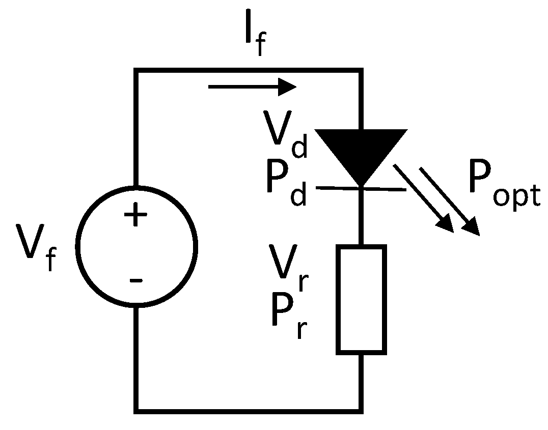
The (total) effective thermal resistance is defined as the ratio R th e ( t ) = Δ T ( t ) / P el , with electric input power P el given as P el = P d + P r , where P r defines the electric loss; see [51]. It is assumed that the total electric power fed into the LED system during power cycling is given as P d = I f · V f . Electric input leaves partly as heat and partly as light; thus, P el = P opt + P heat ; see Figure 2. P opt is the emitted optical power, and P heat remains as dissipated heat. Thus, the investigated model assumes that the device has a constant efficiency η , and the electric loss P r can be neglected, i.e.,  P el = P d . Therefore, P opt = η · P d , which refers to the optical power the LED emits, and, simultaneously, P heat = P d η · P d = P d · ( 1 η ) . Furthermore, with the residual thermal resistance R th ( t ) = Δ T ( t ) / P heat , the effective thermal resistance can be calculated as R th e ( t ) = R th ( t ) P heat / P d = ( 1 η ) R th ( t ) . Hence, the temperature step at power cycle time t can be modelled as
Δ T ( t ) = R th ( t ) · ( 1 η ) · I f · V f
with parameters R th ( t ) , η , I f and V f . The temperature swing results in degradation of materials due to thermal fatigue. Cyclic thermal stresses and strains are induced due to temperature changes, spatial temperature gradients and high temperatures under constrained thermal deformation, resulting in a change of the thermal resistance over time. Thermal stresses are produced by cyclic material expansion and contraction when temperature changes under geometric constraints, such as what happens in LED systems under real operating conditions.
We focus on the initial temperature swing, Δ T t = 0 = Δ T 0 , which is vitally important for the increase of the LED junction temperature swing over the number of power cycles (cf., e.g., [52]), i.e.,
Δ T 0 = R th · η h · I f · V f
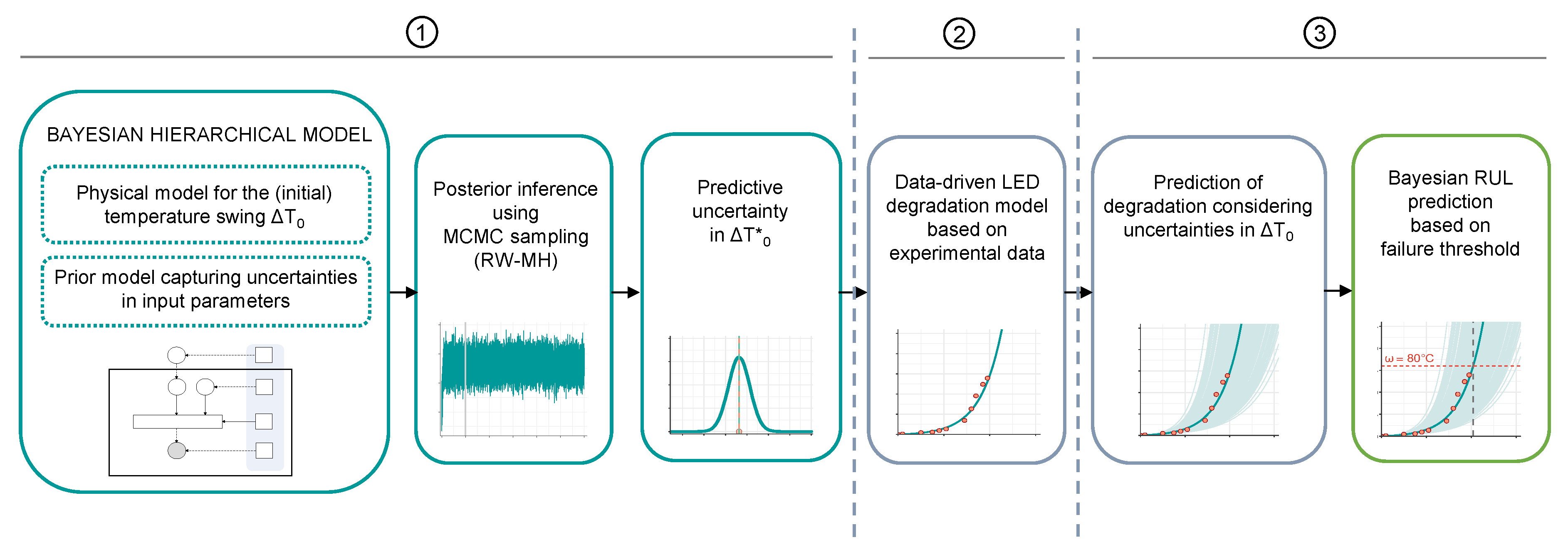
based on the thermal resistance R th (at t = 0 ) and parameters η h = 1 η , I f and V f . Using a probabilistic framework, we systematically account for different types and sources of uncertainty and variability in the input parameters in (2) to quantify the overall uncertainty in Δ T 0 . We present the Bayesian modelling framework in Section 3.2 which is detailed in Section 4 to address different issues that are commonly met in real applications. Based on experimental data, we discuss the potential impact of the uncertainty in Δ T 0 on RUL prediction using an existing lifetime prediction model that relies on the initial temperature swing in Section 6. The procedure is described in Figure 3.

3.2. Bayesian Hierarchical Modelling Framework

A probabilistic framework is a common modelling choice for UQ, since it accounts for randomness and uncertainty in a systematic manner. Based on the physically derived model in (2), we consider a Bayesian hierarchical (multi-level) modelling approach to accommodate different types of uncertainty in the input parameters.

3.2.1. Likelihood Distribution

The deterministic model (2) relates physical input parameters to measurable output quantities. Thus, for given input parameters Θ = ( R th , η h , I f , V f ) ,
M : Θ y ˜ = M ( Θ )
predicts a temperature change y ˜ = Δ T ˜ 0 , where M ( · ) represents a forward operator. In practice, forward model predictions deviate from actually observed values y i = Δ T 0 i , i = 1 , , n , due to measurement noise and randomness in the data-generating process in general, even if all input parameters Θ were perfectly known. Forward model predictions require precise knowledge about the inputs involved. However, model (2) is subject to uncertainties and variabilities through the inputs. In order to learn about these physically fixed, though actually unknown (“uncertain”) forward model parameters from observed data, we consider a classical inversion problem setting. Bayesian methods have become a popular method for UQ in inverse problems (see, e.g., [45,53]); this is also attributed to to their natural mechanism for regularization in typically ill-posed inverse problems [54].
Reformulating (3) as an inverse model, the observed (measured) temperature swing of an LED system i, i = 1 , , n is interpreted as
y i = M ( Θ i ) + ε i , Δ T 0 i = M ( R th i , η h , i , I f , i , V f , i ) + ε i = R th i · η h , i · I f , i · V f , i + ε i ,
where the residuals ε i describe the discrepancy between forward model predictions and observed data. These residuals are commonly assumed to be additive, centred and independently distributed of Θ . A rather simple choice in practice is to assume that
ε i N 0 , σ ε 2
with constant residual variance σ ε 2 . Hence, the likelihood distribution is given by
p ( y | Θ ) = i = 1 n p ( y i | Θ i ) = i = 1 n p ε ( y i M ( R th i , η h , i , I f , i , V f , i ) | σ ε 2 )
assuming conditional independence, i.e., the data are stochastically independent given Θ . The likelihood distribution explains random uncertainty in the observed temperature swings given Θ , which has been induced by measurement noise.

3.2.2. Prior Distributions

Bayesian model specification ends up with an entire probabilistic model in terms of a joint probability distribution for all observable and unobservable quantities in a problem. The uncertainty of the unobserved parameters Θ is modelled by the prior probability distribution p ( Θ ) , which allows incorporation of available prior information from various sources. We take a hierarchical modelling approach that allows to consider different types of physical input parameters in (4) which differ in their level and nature of uncertainty:
  • Deterministic inputs: The parameters η h and V f in (4) are assumed to be perfectly known and are thus considered as deterministic input parameters, i.e., z i = ( η h , i = η h , V f , i = V f ) .
  • Aleatory variability: In general, hierarchically specified prior distributions may be assigned to input parameters that are subject to aleatory variability. We classify these types of parameters into parameters for which (a) randomness is induced by known variability and (b) randomness is induced by variability that is itself unknown. Similar prior considerations are used and discussed in Nagel and Sudret [24] for simply supported beam deflections.
    (a)
    Known variability: We assume that the physically realized currents I f , i in (4) (may) vary randomly between different systems due to some known degree of uncertainty that is inherent to the equipment used. Thus, the hyper-parameters θ I f , i of the prior
    I f , i p ( I f , i | θ I f , i )
    represent available information about the accuracy of the power unit adjusting I f , i . The uncertainty in the realized values I f , i is then “prescribed” by the hyper-parameters θ I f , i ; cf. [24].
    (b)
    Unknown variability: Variabilities in the thermal resistances R th i across identically manufactured LED systems may result either from production (e.g., due to irregularities in the manufacturing process of LED packages) or from the setup or application (e.g., due to the TIM). For both sources, the magnitude of variability is assumed to be unknown. For input parameters with unknown aleatory, the structure of the prior in (7) is extended by another level of hierarchy. We assume that the thermal resistances are subject to this type of “unknown” aleatory variability, and we specify the prior as
    R th i p ( R th i | ϑ R th ) ,
    ϑ R th p ( ϑ R th | γ R th ) ,
    where the hyper-parameters ϑ R th are assigned a hyper-prior given in (9) rather than being fixed with additional hyper-parameters γ R th .
  • Epistemic uncertainty: The hyper-parameters ϑ R th in (9) refer to unknown parameters that are subject to epistemic uncertainty, which is modelled as ϑ R th p ( ϑ R th | γ R th ) .
In general, epistemic uncertainty is reducible in practice with increased knowledge, whereas the aleatory variability in (2a) and (2b) is not. Note also that η h and V f may be subject to variabilities in practice. Then, prior distributions as described in (2a) have to be specified.
We denote by Θ = ( R th , ϑ R th , I f ) the collection of all parameters and hyper-parameters for which a prior distribution has to be specified. We assume conditional prior independence, and hence, the joint prior of Θ is given by
Θ = i = 1 n p ( I f , i | θ I f , i ) i = 1 n p ( R th i | ϑ R th ) p ( ϑ R th | γ R th ) .
We give details on the specific prior distributions in Section 4.2, Section 4.3 and Section 4.4.

3.2.3. Bayesian Hierarchical Model

Having specified the likelihood distribution and the priors, the overall Bayesian hierarchical (or multi-level) model is summarized in the following way:
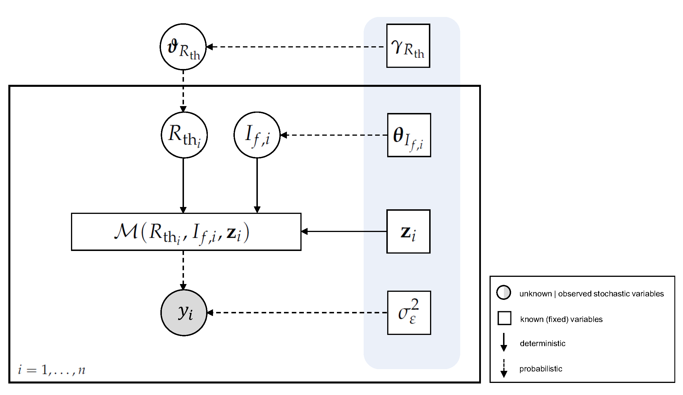
y i | R th i , I f , i , z i p ( y i M ( R th i , I f , i , z i ) | σ ε 2 ) R th i p ( R th i | ϑ R th ) ϑ R th p ( ϑ R th | γ R th ) I f , i p ( I f , i | θ I f , i )
with z i = ( η h , V f ) , and it can be represented as a probabilistic graphical model (PGM), cf. [55,56,57]), or, more specifically, as a directed acyclic graph (DAG), also known as Bayesian network (BN) [58]. The joint posterior distribution of the unknown parameters Θ = ( R th , ϑ R th , I f ) is obtained by combining the likelihood in (6) and the joint prior (10) into the posterior distribution, i.e.,
p ( R th , ϑ R th , I f | y ) = 1 C i = 1 n p ( y i | R th i , I f i , z i ) · i = 1 n p ( I f , i | θ I f , i ) · i = 1 n p ( R th i | ϑ R th ) · p ( ϑ R th ) .
The normalizing constant C of the posterior is given as
C = I f n R th n ϑ R th p ( R th , ϑ R th , I f | y ) d I f d R th d ϑ R th .
Based on (12), inference on specific parameters of interest can be achieved by marginalization. The corresponding DAG representation of the joint posterior is shown in Figure 4.
It provides a model representation for the hierarchical structure of the joint probability distribution over a set of random variables in terms of prior and conditional distributions, linking parameters, hyper-parameters and the observed data by using concepts of graph theory and conditional independence among random variables; see [24,59].
The posterior distribution in (12) accounts for random uncertainty in the generated data, induced, e.g., by measurement noise, through the likelihood as well as for epistemic parameter uncertainty via the prior. Thus, exploring the posterior distribution opens up a natural framework for UQ by computing credible intervals and posterior predictive distributions. Posterior uncertainty related to Θ can be quantified using credible regions based on quantiles of the posterior distribution; cf. [22]. Uncertainty in the prediction of future observations y * is fully considered within the Bayesian framework by providing the posterior predictive distribution p ( y * | y ) , which quantifies the predictive uncertainty in y = Δ T 0 and is given as
p ( y * | y ) = Θ p ( y * | Θ , z ) · p ( Θ | y , z ) d Θ .
See, e.g., [23,60] for details. Hence, the posterior predictive distribution reflects two types of uncertainty: the uncertainty in sampling future data (sampling uncertainty) through p ( y * | Θ , z ) , and parametric (estimation) uncertainty about Θ through the posterior distribution, i.e.,  p ( Θ | y , z ) .

3.3. Posterior Inference

Bayesian inference is performed by summarizing the posterior distribution in (12), which is analytically intractable. We take a sampling-based MCMC approach for posterior inference using a block-wise random-walk Metropolis–Hastings (RW–MH) algorithm; see [61,62] for details. The basic idea of MH algorithms is to build a Markov chain with the target posterior distribution as its stationary distribution. The implementation of a MH sampler is based on the choice of suitable proposal distributions for the parameters, from which candidates for the Markov chain are sampled.
We use block-wise sampling by grouping the parameters of interest, i.e., R th , i , ϑ R th and I f , i , into blocks, and we use Gaussian proposal distributions in each block, centred around the previous value of the chain. The variance parameter of the proposal distributions is tuned to achieve block-wise acceptance rates (i.e., proportion of candidate values that is accepted during MCMC sampling) between 20% and 40%, which proves well for random-walk proposals; cf. [24,63,64]. The MCMC sampling scheme is implemented in R [65]. Algorithm 1 outlines the sampling steps to generate samples from the hierarchical posterior distribution.
Given the MCMC samples from the posterior distribution, i.e., Θ i ( m ) p ( Θ i | y i ) , for  m = 1 , , M , samples from the posterior predictive distribution can be obtained as
y i * ( m ) = Δ T 0 i * ( m ) p ( y i | Θ i ( m ) , z i )
based on draws from the sampling distribution specified in (6).
Algorithm 1 RW–MH algorithm for posterior sampling.
1: Given the current state m = 1 , , M of the Markov chain for the parameters Θ k ( m ) of the kth block, k = 1 , , 3 , a candidate is sampled from the proposal distribution
Θ k ( m + 1 ) q Θ k ( m + 1 ) | Θ k ( m ) , Θ k ( m )
given by a Gaussian distribution centred around the current value Θ k ( m ) and the variance ϵ 2 I d , where ϵ is a tuning parameter, and I d is the d-dimensional identity matrix of dimension d of the parameter vector of the respective block. The parameter vector Θ k ( m ) denotes all parameters except for those summarized in block Θ k ( m ) .
2: The proposed state is accepted if
U j α Θ k ( m + 1 ) | Θ k ( m )
with acceptance probability α ( · ) , which simplifies to
α Θ k ( m + 1 ) | Θ k ( m ) = min 1 , p ( Θ k ( m + 1 ) , Θ k ( m ) | y ) p ( Θ k ( m ) , Θ k ( m ) | y )
and U j is a random draw from U [ 0 , 1 ] .
Otherwise, the proposed value is rejected, i.e.,  Θ k ( m + 1 ) = Θ k ( m ) .

4. Simulation Experiments

To investigate the performance of the proposed MCMC method to sample from the posterior in (12), we consider simulated data of identically manufactured LED systems. Test data generation is described in Section 4.1. The test datasets are used to address different experimental scenarios that are commonly encountered in applications:
  • Issue 1: Production and application variability (Section 4.2). In practice, we are primarily interested in the variability within the thermal resistances across the sample of “identically” manufactured LED systems due to material (production) and setup (application) variability. Thus, inference focuses on the estimation of the hyper-parameters ϑ R th = ( μ R th , σ R th ) which determine the variability in R th i . The thermal resistances themselves are not of immediate interest and are considered nuisance. Analyses on this default issue are based on data from experiment E1.
  • Issue 2: Measurement uncertainty (Section 4.3) deals with a modification of Issue 1 by considering unknown residual variances σ ε 2 . The default model is extended to additionally estimate the variance parameter. The same datasets as in Issue 1 are used for implementation of Issue 2.
  • Issue 3: Uncertain experimental conditions (Section 4.4). In addition to the default setting in Issue 1, we also consider varying operational conditions by assuming that the realized forward currents I f , i vary between the LED systems; see prior type 2a in Section 3.2.2. The primary aim here is to quantify the impact of this uncertainty on the quantities of interest ϑ R th = ( μ R th , σ R th ) . Modifications of the algorithm proposed for Issue 1 are straightforward. Experiment E3 points out different strategies in dealing with uncertain conditions.

4.1. Test Datasets

Different experiments are assigned to the problem setups above to show how these issues can be addressed in applications.
Experiment 1 (E1): In the default setting, the proportion of input power which remains as heat, i.e., P heat = I f · V f · η h , is well-known. The LED systems are exposed to electric input power with forward current I f = 0.68 A and forward voltage V f = 11.909 V. The amount of input power that is converted to heat is assumed to be fixed at η h = 0.35 . The simulated LED systems are similar insofar that we assume variability in R th i . Thus, for i = 1 , , n , the total thermal resistances R th i are sampled from a lognormal distribution with parameters μ R th = 39.13 K/W and σ R th = 1 K/W, which corresponds to measurements of a (specimen) LED system in the experimental setup used in Magnien et al. [52].
For i = 1 , , n , the temperature swing at starting, y ˜ i = Δ T ˜ 0 i , is computed according to (2) and perturbed by a noise term ε i N 0 , σ ε 2 with 0.5 °C to account for measurement uncertainty and imperfection of the physical forward model. We generate 100 datasets each for different sample sizes n j , j = 1 , 2 , 3 , with n 1 = 20 , n 2 = 100 and n 3 = 500 to assess the impact of an increasing number of observations on the performance of the method.
Experiment 2 (E2): The same test datasets as in E1 are used to address unknown measurement uncertainty.
Experiment 3 (E3): In contrast to E1, the physically realized currents are not constant, but may deviate from the set target value due to some amount of known uncertainty in the equipment used; cf. [66]; see Section 3.2.2, type 2a. We generate another 100 test datasets each with n = 100 identically manufactured LED systems as in E1, except that now we assume variability within I f , i , i = 1 , , n . Thus, currents are independently sampled from a normal distribution with μ I f = 0.68 A and σ I f = 0.034 A, which corresponds to a coefficient of variation of 5%. Experiment 3 strives to quantify the impact of prescribed uncertainty in I f , i on ϑ R th by considering different strategies for dealing with variability within I f , i :
E3.a 
Idealized strategy: We assume that the actually realized, though random, currents are perfectly known and set to the true values I f , i = I f , i true , i = 1 , , n used to generate the datasets. Obviously, this first strategy is an idealized (hypothetical) and unrealistic scenario in applications. However, it will be used as a reference (benchmark) for comparison with the other strategies.
E3.b 
Ignorant strategy: Potential variability is totally ignored within the applied currents, which are taken to be fixed at their targeted values, i.e., I f , i = I f = 0.68 A. While the data have been generated under I f , i true , the analysis is performed under I f , i = I f . This is probably a common scenario in practice, when variabilities in physical experiments are not considered.
E3.c 
Proper treatment strategy: The aleatory variability in the physically realized currents is taken into account by treating I f , i as an unknown parameter and assigning a prior distribution for I f , i as in (7).

4.2. Issue 1: Production and Application Variability

The first issue aims at quantifying the variability within the module-specific thermal resistances R th i assuming σ ε 2 is known. The parameters η h , I f and V f are treated as deterministic input parameters, which refers to type 1 parameters; see Section 3.2.2. The individual thermal resistances R th i and the hyper-parameters ϑ R t h are treated as unknowns, i.e., Θ 1 = ( R th i , ϑ R th ) . Following (4), we assume
y i = Δ T 0 i = M R th i , z i + ε i , ε i N 0 , σ ε 2
with deterministic parameters z i = ( I f , V f , η h ) .
We use a lognormal prior for the thermal resistances, i.e., R th i LN ( μ R th , σ R th ) ; see (8) of type 2b parameters in Section 3.2.2. The hyper-parameters ϑ R th = ( μ R th , σ R th ) are assigned uniform prior distributions μ R th U [ m l , m u ] and σ R th U [ s l , s u ] . For the parameters of the prior distributions, we choose m l = 0 , m u = 100 , s l = 0 and s u = 10 to specify weakly informative, flat priors with predefined lower and upper bounds.
The joint (non-normalized) posterior distribution of Θ 1 = ( R th i , μ R th , σ R th ) is given as
p ( R th , ϑ R th | y ) i = 1 n p ( y i | R th i , z i ) · i = 1 n p ( R th i | μ R th , σ R th ) · p ( μ R th ) · p ( σ R th ) .
According to the hierarchical structure of the target distribution, the RW–MH sampler for this default setting consists of two blocks, i.e., the individual thermal resistances R th , i and the parameters ϑ R th = ( μ R th , σ R th ) .

4.3. Issue 2: Unknown Measurement Uncertainty

The second issue considers the same setting as in Section 4.2 except the residual variance σ ε 2 is assumed to be unknown. We assign a Beta prior to the parameter σ ε , i.e., σ ε B ( a 0 , b 0 ) . We assume that prior information about the measurement uncertainty σ ε is available from repeatability testing, and we specify the hyper-parameters of the Beta prior for σ ε accordingly to reflect prior knowledge of σ ˜ ε 0.5 °C ± 0.1 °C, i.e., by specifying a 0 = 12 , b 0 = 12 ; cf. [67]. The resulting (non-normalized) joint posterior distribution of the unknown parameters Θ 2 = ( R th , ϑ R th , σ ε ) is extended to
p ( R th , ϑ R th , σ ε | y ) i = 1 n p ( y i | R th i , z i , σ ε ) · i = 1 n p ( R th i | μ R th , σ R th ) p ( μ R th ) · p ( σ R th ) · p ( σ ε )
with z i = ( I f , V f , η h ) . Modifications of the MCMC sampling scheme are straightforward and include an additional block to sample the parameter σ ε .

4.4. Issue 3: Uncertainty in Experimental Conditions

Implementation of E3.a and E3.b is analogous to Issue 1. Inference is based on the posterior in (16) with z i = ( I f , i true , V f , η h ) for E3.a and z i = ( I f , i = I f , V f , η h ) for E3.b, with the difference being that the data have been generated with random I f , i , instead of I f . Pursuing production and application variability (Issue 1) in the presence of uncertainty in the experimental condition, a prior distribution for I f , i is specified as in (7), where p ( I f , i | θ I f , i ) N ( μ I f , σ I f 2 ) with known hyper-parameters θ I f , i = θ I f = ( μ I f , σ I f ) . The parameter σ I f refers to the degree of uncertainty induced by the equipment used to adjust the current. We assume that information on σ I f is provided by the product datasheet of the power unit; cf. [66]. The joint (non-normalized) posterior in (16) is extended to
p ( R th , ϑ R th , I f | y ) i = 1 n p ( y i | R th i , I f , i , z i ) · i = 1 n p ( I f , i | μ I f , σ I f ) · i = 1 n p ( R th i | μ R th , σ R th ) · p ( μ R th ) · p ( σ R th )
with z i = ( V f , η h ) and corresponds to (12). The MCMC sampling scheme in Section 4.2 is extended by an additional block to sample the unknown parameters Θ 3 = ( R th , ϑ R th , I f ) . Again, the thermal resistances and the currents are not of immediate interest and are considered nuisances. The primary focus is on the estimation of parameters μ R th and σ R th .

5. Results and Discussion

In this section, the results for Issues 1–3 based on experiments E1–3 are discussed.

5.1. Issue 1: Production and Application Variability

Parameter estimation of Θ 1 is performed according to the block-wise implemented RW–MH algorithm outlined in Algorithm 1 based on (16). For each dataset in E1, MCMC was run for 100,000 iterations after a burn-in phase of 20,000 draws with a thinning of 10 (i.e., 10,000 iterations are retained by keeping only every 10th draw). We performed a number of convergence checks to assess the convergence behaviour of the Markov chain by visualizing the output using trace plots and autocorrelation function (ACF) plots of the MCMC samples; see Figure 5. Convergence to the posterior distribution is apparent from the left side of Figure 5. Additionally, the ACF of the thinned samples (after having discarded the draws of the burn-in phase) quickly decays after only a few lags. Mixing and efficiency of the MH algorithm was also evaluated on the basis of the effective sample size (ESS) and the integrated autocorrelation time (IAT); cf. [68] for details.
The resulting posterior marginal distributions for μ R th and σ R th for one dataset of E1 are shown in Figure 6. The estimated variability in R th within a sample of n 2 = 100 LED systems, which is captured by σ R th , shows a good match with the true value.
Table 1 summarizes the results for the test data of E1 (see I1). We report the average of the posterior means of parameters μ R th and σ R th , the average of the 95% highest posterior density (HPD) regions and the length of the average 95%-HPD regions over 100 datasets based on different sample sizes n 1 = 20 , n 2 = 100 and n 3 = 500 . The mean and the standard deviation of the thermal resistances are well-estimated, with averaged posterior means being close to the true values that were used to generate the data. As expected, performance improves with increasing sample size. Thus, the posterior uncertainty estimated by the averaged 95%-HPD intervals steadily decreases with an increasing number of observations, which is directly evident from the HPD lengths. Providing more knowledge in the form of more data, the epistemic uncertainty in ϑ R th can be reduced by learning about ϑ R th from the data. This gain in precision is graphically displayed in Figure 7.
Uncertainty in the prediction of future observations is accounted for in the posterior predictive distribution p ( Δ T 0 i * | Δ T 0 i ) , i = 1 , , n in (14), which is illustrated for one dataset of E1 in Figure 8 (right). The posterior predictive distribution is obtained based on samples from the marginal posterior distribution of the nuisance parameter R th i , which is shown on the left side of Figure 8.

5.2. Issue 2: Measurement Uncertainty

To account for unknown measurement uncertainty, the parameters Θ 2 are sampled from the modified posterior distribution in (17). The simulation results for Issue 2, averaged over 100 datasets, are summarized in Table 1 (see, I2), where the averaged posterior estimates for the residual standard deviation are additionally included. Again, the posterior uncertainty in the estimated model parameters decreases for larger sample sizes. From Table 1, we also conclude that introducing additional uncertainty in the residual model does not affect the inference of the quantities of interest μ R t h and σ R th . The averaged posterior means for μ R th and σ R th are very similar in both scenarios, I1 and I2.
Figure 9 shows the posterior distribution for σ ε for one dataset based on n 2 = 100 and n 3 = 500 LED systems and on different prior distributions. Obviously, the amount of prior knowledge, e.g., provided by repeatability testing, and the sample size affect the amount of posterior uncertainty in σ ε .

5.3. Issue 3: Uncertain Experimental Conditions

The setup in E3 aims to compare different strategies for dealing with uncertain experimental conditions. As with the previous issues, MCMC was run for 100,000 iterations with a burn-in of 20,000 iterations and a thinning of 10 for strategies E3.a and E3.b to estimate the parameters μ R th and σ R th . For each dataset, the modified MCMC algorithm in E3.c was run for 200,000 iterations after a burn-in of 100,000 draws with a thinning of 10 to ensure convergence to the target distribution. Results are summarized in Table 2, where the averaged posterior means for ϑ R th under the three strategies and the averaged lower and upper bounds of 95%-HPD regions and the respective averaged 95%-HPD region lengths over 100 datasets of size n = 100 are reported.
Figure 10 illustrates the distribution of the averaged posterior means for ϑ R th over the simulated datasets for the three strategies, where the first (idealized) one serves as the reference (“what if”) strategy. Averages of the posterior means for μ R th agree well with the true values under all strategies, but E3.b (ignorant) and E3.c (proper) show considerably more variation than E3.a (idealized). This is also evident from the respective length of the averaged 95%-HPD regions.
However, for the variance parameter σ R th , we observe a different result. If aleatory variability in the experimental setup is not taken into account and the currents are erroneously taken on their targeted values (E3.b), we get misleading estimates of the posterior mean for σ R th . Thus, the additional variability in the observed data induced by the equipment used is apparently attributed to σ R th , over-estimating the variability within the thermal resistances. Consequently, inference of the predictive distribution for Δ T 0 i will be biased. In contrast, if the variability in the currents is properly considered by treating them as uncertain (E3.c), we observe that the posterior means are much closer to the true value, but the additional variability in the currents has increased the level of estimation uncertainty.

6. Application Scenario Based on Measured Temperature Data

The lifetime and reliability of LED systems crucially depends on the thermal stress the system is exposed to under thermal cyclic loading. If the LED junction temperature swing exceeds a certain (failure) threshold, the LED package is susceptible to failures and has to be replaced. Thus, accurate quantification of the system’s predicted lifetime is important to ensure safe and reliable operation. Bayesian approaches to RUL prediction of LED systems effectively deal with parameter uncertainties in the degradation model, thus leading to more accurate and stable lifetime predictions. In an application scenario based on measured temperature data available from [43,52] (see Figure 11), we study the possible impact of the results obtained from Section 5 on RUL prediction using the degradation model proposed in [43].

6.1. Bayesian RUL Prediction

Following the thermal impedance monitoring model in Magnien et al. [52], a data-driven approach is used to model the increase in the junction temperature change Δ T j over the PC runtime for RUL prediction of an LED system. There, the change of temperature and the change in thermal resistance over time are modelled by the use of a power law, which is typically applied for cyclic loading, and an Arrhenius model used for temperature-driven ageing behaviour. The combination of both enables the description of solder fatigue over the PC runtime.
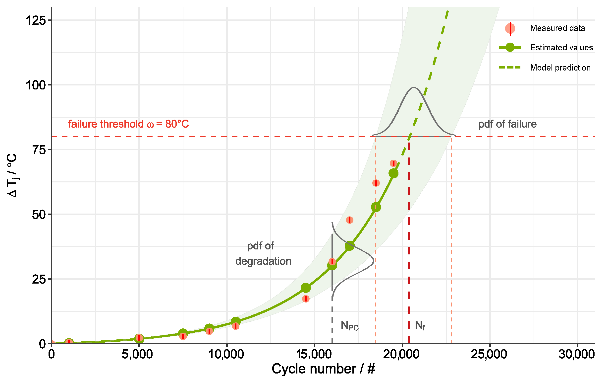
Bayesian regression modelling is performed as proposed in Magnien et al. [43] to model the increase in Δ T j depending on a (fixed) temperature swing at the initial state Δ T 0 and the number of cycles performed ( N PC ) using a linearisation of the approximation provided in [52] (Equation (2)). The approach in [43] handles the epistemic uncertainty in unknown model parameters, and thus allows more accurate RUL prediction of the system. However, potential variability stemming from production or operation is not considered due to the unavailability of relevant data. The resulting model predictions with 95% credible intervals for an LED system with fixed Δ T 0 = 110.92 °C are shown in Figure 12.
Taking a probabilistic approach allows quantification of the degradation level at any specific cycle number N PC via the probability density function (pdf) of Δ T j and the corresponding credible region of the predicted junction temperature change. This pdf can further be used to determine the pdf of failure, N f , and the RUL, which is defined as the remaining lifetime (time to failure) until the expected temperature swing Δ T j reaches a failure threshold ω ; cf. [37]. An LED system is considered failed when the LED junction temperature swing exceeds ω = 80 °C; cf. [52]. Additionally, the boundaries of the 95% credible interval for the number of cycles N PC = N f enable more accurate quantification of the predicted time to failure.

6.2. Impact of Input Uncertainty on Bayesian RUL Prediction

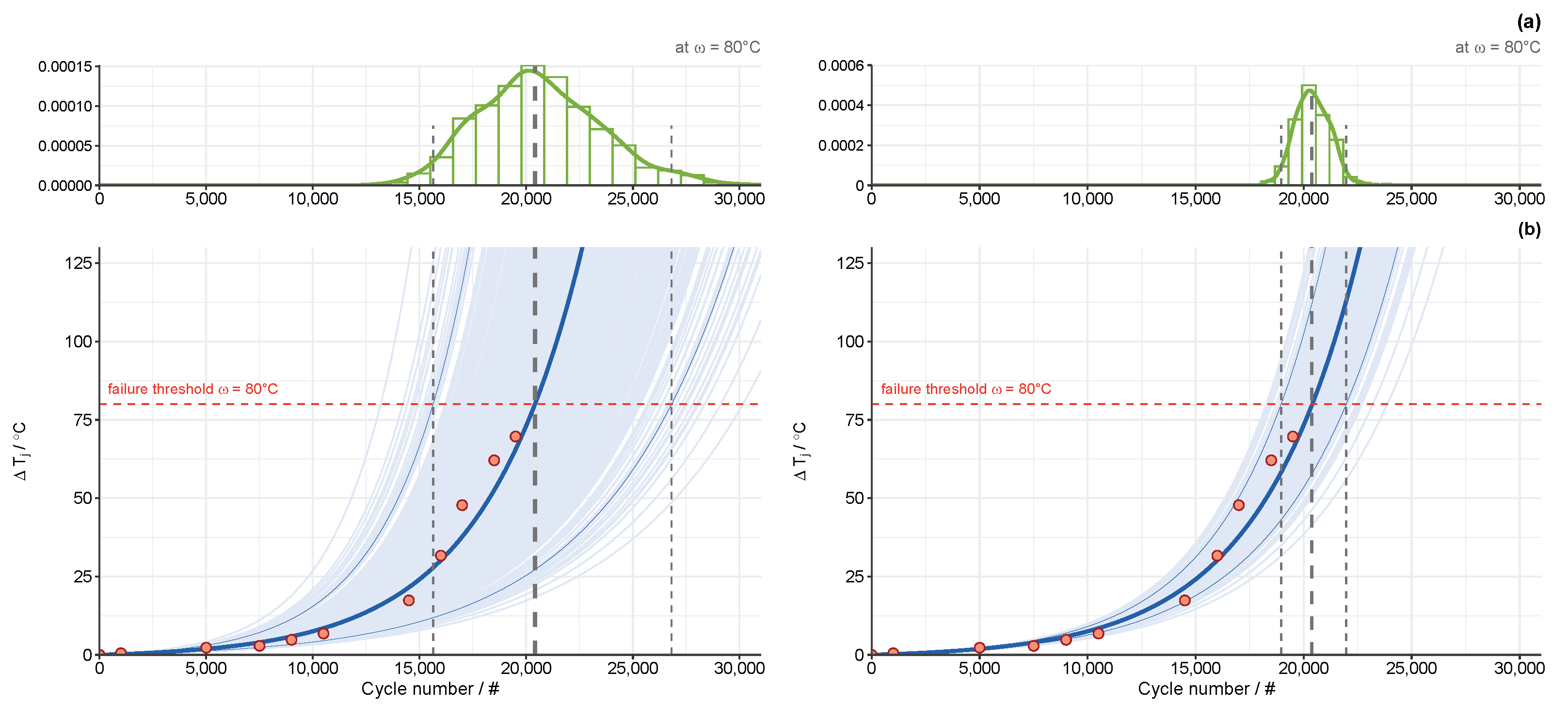
RUL prediction in Figure 12 is based on a fixed starting temperature swing of Δ T 0 = 110.92 °C measured for the LED system that served as the specimen system in the test data simulation in Section 4. Using the predictive distribution of Δ T 0 obtained from Section 5.1 (based on E1) instead of Δ T 0 , we aim at studying the impact of production and application variability in Δ T 0 on RUL prediction. Figure 13b shows the resulting predicted increase in Δ T j over the PC runtime based on test data of n 3 = 500 LED systems with different variability within the thermal resistances, i.e., σ R th = 1 K/W and σ R th = 0.3 K/W. Additionally, Figure 13a compares the respective pdfs of failure.
For σ R th = 1 K/W, the number of cycles until the predicted temperature swing reaches the failure threshold is estimated at N f = 20 , 638 (median 20,413). The corresponding lower and upper limits of the 95% credible interval are [ 15 , 636 ; 26 , 813 ] cycles. For less variability within the thermal resistances, σ R th = 0.3 K/W, the predicted time to failure is 20,416 cycles (median 20,378), with a narrower credible region of [ 18 , 956 ; 21 , 971 ] power cycles. Obviously, inherent uncertainty in the initial temperature swing has a considerable impact on the resulting uncertainty in RUL prediction, and its variability decreases with decreasing variability in σ R th . Thus, sources of potential uncertainty of the system in focus have to be carefully considered for RUL prediction to be reliable. Beyond the quantification of uncertainty, from Figure 13, the need also arises to deal with the variability σ R th to reduce the uncertainty on the RUL.

7. Conclusions

In this paper, a comprehensive probabilistic framework has been developed to account for different types of uncertainty in input parameters of a physical model describing the temperature swing of an LED system under thermal stress. The presented hierarchical approach relies on an inverse problem formulation of the physically derived model for which the Bayesian paradigm provides a well-suited mechanism for regularization and UQ. The focus has been on the overall uncertainty in the initial temperature swing an LED system is exposed to during PC testing. Variability within the generated initial temperature swings is mainly caused by variability within the operational thermal resistances of the LED systems, but also measurement and operating uncertainty have been taken into consideration. For posterior inference, a block-wise RW-MH algorithm has been implemented in the statistical software R. Performance of the proposed method has been illustrated for simulated data which address different issues in practice. It has been shown that potential variability inherent in measured temperatures of supposedly identical LED systems can be attributed to variability in their operational thermal resistances. This uncertainty may have a non-negligible impact on the prediction of their possible service life, when being disregarded in lifetime prediction models. Findings from an application scenario in which the results for the LED test data are used to study their impact on RUL have highlighted the need for a comprehensive quantification and management of uncertainties in applications to allow for reliable predictions.

Author Contributions

Conceptualization, M.D., J.M. and M.M.; methodology, M.D., J.M. and U.K.; software, M.D.; validation, M.D. and J.M.; investigation, M.D. and J.M.; data curation, M.D.; writing—original draft preparation, M.D. and J.M.; writing—review and editing, M.D., J.M., U.K, E.K. and M.M.; visualization, M.D. and J.M.; project administration, M.M. and J.M. All authors have read and agreed to the published version of the manuscript.

Funding

The authors gratefully acknowledge the financial support under the scope of the COMET program within the K2 Center “Integrated Computational Material, Process and Product Engineering (IC-MPPE)” (project no. 886385). This program is supported by the Austrian Federal Ministries for Climate Action, Environment, Energy, Mobility, Innovation and Technology (BMK) and for Digital and Economic Affairs (BMDW), represented by the Austrian Research Promotion Agency (FFG) and the federal states of Styria, Upper Austria and Tyrol.

Institutional Review Board Statement

Not applicable.

Informed Consent Statement

Not applicable.

Data Availability Statement

The simulated data presented in this paper are available on request from the corresponding author.

Conflicts of Interest

The authors declare no conflict of interest.

References

  1. Yazdan Mehr, M.; Bahrami, A.; van Driel, W.D.; Fan, X.J.; Davis, J.L.; Zhang, G.Q. Degradation of optical materials in solid-state lighting systems. Int. Mater. Rev. 2020, 65, 102–128. [Google Scholar] [CrossRef] [Green Version]
  2. Caers, J.F.J.M.; Zhao, X.J. Failure Modes and Failure Analysis. In Solid State Lighting Reliability: Components to System; van Driel, W.D., Fan, X.J., Eds.; Springer: New York, NY, USA, 2013; pp. 111–184. ISBN 978-1-4614-3067-4. [Google Scholar]
  3. Chang, M.-H.; Das, D.; Varde, P.V.; Pecht, M. Light emitting diodes reliability review. Microelectron. Reliab. 2012, 52, 762–782. [Google Scholar] [CrossRef]
  4. Pecht, M.G.; Chang, M.H. Failure Mechanisms and Reliability Issues in LEDs. In Solid State Lighting Reliability: Components to System; van Driel, W.D., Fan, X., Eds.; Springer: New York, NY, USA, 2013; pp. 43–110. ISBN 978-1-4614-3066-7. [Google Scholar]
  5. Arques-Orobon, F.J.; Nuñez, N.; Vazquez, M.; Segura-Antunez, C.; González-Posadas, V. High-power UV-LED degradation: Continuous and cycled working condition influence. Solid-State Electron. 2015, 111, 111–117. [Google Scholar] [CrossRef] [Green Version]
  6. Narendran, N.; Liu, Y.; Mou, X.; Thotagamuwa, D.R. Predicting LED system life: A long-term study of the factors that determine performance and failure. In Proceedings of the IES 2017 Annual Conference, Portland, OR, USA, 10–12 August 2017. [Google Scholar]
  7. Narendran, N.; Liu, Y.; Mou, X.; Thotagamuwa, D.R.; Eshwarage, O.V.M. Projecting LED product life based on application. In Proceedings of the 15th International Conference on Solid State Lighting and LED-based Illumination Systems, San Diego, CA, USA, 14 September 2016. [Google Scholar] [CrossRef]
  8. Qian, C.; Fan, X.J.; Fan, J.J.; Yuan, C.A.; Zhang, G.Q. An accelerated test method of luminous flux depreciation for LED luminaires and lamps. Reliab. Eng. Syst. Saf. 2016, 147, 84–92. [Google Scholar] [CrossRef]
  9. Hillman, C.; Serebreni, M.; Blattau, N.; Bhatkal, R.; Dutt, G.; Pandher, R. Fatigue Life Prediction Model for LEDs on Metal Core Printed Circuit Boards (MCPCBs) with Pb-Free Solder Alloys. In Proceedings of the SMTA International Conference 2017, Rosemont, IL, USA, 17–21 September 2017; Volume 1, ISBN 9781510849365. [Google Scholar]
  10. Durand, C.; Klingler, M.; Coutellier, D.; Naceur, H. Power Cycling Reliability of Power Module: A Survey. IEEE Trans. Device Mater. Reliab. 2016, 16, 80–97. [Google Scholar] [CrossRef]
  11. Siddique, T.; Mahmud, M.S.; Keesee, A.M.; Ngwira, C.M.; Connor, H. A Survey of Uncertainty Quantification in Machine Learning for Space Weather Prediction. Geosciences 2022, 12, 27:1–27:23. [Google Scholar] [CrossRef]
  12. Walker, W.E.; Harremoës, P.; Rotmans, J.; van der Sluijs, J.P.; van Asselt, M.B.A.; Janssen, P.; Krayer von Krauss, M.P. Defining Uncertainty: A Conceptual Basis for Uncertainty Management in Model-Based Decision Support. Integr. Assess. 2003, 4, 5–17. [Google Scholar] [CrossRef] [Green Version]
  13. Ayyub, B.M.; Klir, G.J. Uncertainty Modeling and Analysis in Engineering and the Sciences, 1st ed.; Chapman & Hall, CRC: Boca Raton, FL, USA, 2006; ISBN 9781584886440. [Google Scholar]
  14. Kiureghian, A.D.; Ditlevsen, O. Aleatory or epistemic? Does it matter? Struct. Saf. 2009, 31, 105–112. [Google Scholar] [CrossRef]
  15. Sullivan, T.J. Introduction to Uncertainty Quantification; Springer: Cham, Switzerland, 2015; ISBN 978-3-319-23395-6. [Google Scholar]
  16. Zhang, J.; Yin, J.; Wang, R. Basic Framework and Main Methods of Uncertainty Quantification. Math. Probl. Eng. 2020, 2020, 6068203:1–6068203:18. [Google Scholar] [CrossRef]
  17. Fink, O.; Wang, Q.; Svensén, M.; Dersin, P.; Lee, W.; Ducoffe, M. Potential, challenges and future directions for deep learning in prognostics and health management applications. Eng. Appl. Artif. Intell. 2020, 92, 103678. [Google Scholar] [CrossRef]
  18. Sankararaman, S.; Mahadevan, S.; Orchard, M.E. Uncertainty in PHM. Int. J. Progn. Health Manag. Spec. Issue Uncertain. PHM 2015, 6. [Google Scholar] [CrossRef]
  19. Berger, J.O. Statistical Decision Theory and Bayesian Analysis; Springer: New York, NY, USA, 1985; ISBN 978-1-4757-4286-2. [Google Scholar]
  20. Lee, P.M. Bayesian Statistics: An Introduction, 4th ed.; John Wiley & Sons: Chichester, UK, 2012; ISBN 9781118332573. [Google Scholar]
  21. Robert, C.P. The Bayesian Choice: From Decision-Theoretic Foundations to Computational Implementation, 2nd ed.; Springer: New York, NY, USA, 2007; ISBN 9780387715988. [Google Scholar]
  22. Box, G.E.P.; Tiao, G.C. Bayesian Inference in Statistical Analysis, 1st ed.; Addison-Wesley: Reading, MA, USA, 1973; ISBN 978-0-471-57428-6. [Google Scholar]
  23. Gelman, A.; Carlin, J.B.; Stern, H.S.; Dunson, D.B.; Vehtari, A.; Rubin, D.B. Bayesian Data Analysis, 3rd ed.; Chapman & Hall/CRC Press: Boca Raton, FL, USA, 2013; ISBN 978-1-439-84095-5. [Google Scholar]
  24. Nagel, J.B.; Sudret, B. A unified framework for multilevel uncertainty quantification in Bayesian inverse problems. Probabilistic Eng. Mech. 2016, 43, 68–84. [Google Scholar] [CrossRef] [Green Version]
  25. Wikle, C. Hierarchical Models for Uncertainty Quantification: An Overview. In Handbook of Uncertainty Quantification; Ghanem, R., Higdon, D., Owhadi, H., Eds.; Springer: Cham, Switzerland, 2015; ISBN 978-3-319-11259-6. [Google Scholar]
  26. Hamada, M.S.; Wilson, A.G.; Reese, C.S.; Martz, H.F. Bayesian Reliability; Springer Series in Statistics: New York, NY, USA, 2010; ISBN 978-1-4419-2673-9. [Google Scholar]
  27. Andrade, A.R.; Teixeira, P.F. Statistical modelling of railway track geometry degradation using Hierarchical Bayesian models. Reliab. Eng. Syst. Saf. 2015, 142, 169–183. [Google Scholar] [CrossRef] [Green Version]
  28. Dai, X.; Qu, S.; Sui, H.; Wu, P. Reliability modelling of wheel wear deterioration using conditional bivariate gamma processes and Bayesian hierarchical models. Reliab. Eng. Syst. Saf. 2022, 226, 108710. [Google Scholar] [CrossRef]
  29. Mishra, M.; Martinsson, J.; Rantatalo, M.; Goebel, K. Bayesian hierarchical model-based prognostics for lithium-ion batteries. Reliab. Eng. Syst. Saf. 2018, 172, 25–35. [Google Scholar] [CrossRef]
  30. Wu, J.; Butler, A.; Mueller, M.A.; Mostafa, K. Combining fatigue analysis information into reliability analysis using Bayesian hierarchical modelling method. In Proceedings of the Annual Reliability and Mainainability Symposium (RAMS), Orlando, FL, USA, 23–26 January 2017; pp. 1–7. [Google Scholar] [CrossRef]
  31. Ferreira, C.; Gonçalves, G. Remaining Useful Life prediction and challenges: A literature review on the use of Machine Learning Methods. J. Manuf. Syst. 2022, 63, 550–562. [Google Scholar] [CrossRef]
  32. Si, X.-S.; Wang, W.; Hu, C.-H.; Zhou, D.-H. Remaining useful life estimation - A review on the statistical data driven approaches. Eur. J. Oper. Res. 2011, 213, 1–14. [Google Scholar] [CrossRef]
  33. Ibrahim, M.S.; Fan, J.; Yung, W.K.C.; Prisacaru, A.; Driel, W.; Fan, X.; Zhang, G. Machine Learning and Digital Twin Driven Diagnostics and Prognostics of Light-Emitting Diodes. Laser Photonics Rev. 2020, 14, 200254:1–200254:33. [Google Scholar] [CrossRef]
  34. Fan, J.; Yung, K.C.; Pecht, M. Lifetime estimation of high-power white LED using degradation-data-driven method. IEEE Trans. Device Mater. Reliab. 2012, 12, 470–477. [Google Scholar] [CrossRef]
  35. Sutharssan, T.; Stoyanov, S.; Bailey, C.; Rosunally, Y. Prognostics and Health Monitoring of High Power LED. Micromachines 2012, 3, 78–100. [Google Scholar] [CrossRef] [Green Version]
  36. Wen, M.; Jing, Z.; Ibrahim, M.S.; Fan, J.; Zhang, G. A hybrid degradation modeling of light-emitting diode using permutation entropy and data-driven methods. In Proceedings of the 22nd International Conference on Electronic Packaging Technology (ICEPT), Xiamen, China, 14–17 September 2021; pp. 1–6. [Google Scholar] [CrossRef]
  37. Zhao, S.; Blaabjerg, F.; Wang, H. An Overview of Artificial Intelligence Applications for Power Electronics. IEEE Trans. Power Electron. 2021, 36, 4633–4658. [Google Scholar] [CrossRef]
  38. Li, M.; Meeker, W.Q. Application of Bayesian Methods in Reliability Data Analyses. J. Qual. Technol. 2014, 46, 1–23. [Google Scholar] [CrossRef]
  39. Lall, P.; Zhang, H. Assessment of lumen degradation and remaining life of light-emitting diodes using physics-based indicators and particle filter. AMSE J. Electron. Packag. 2015, 137, 021002:1–021002:10. [Google Scholar] [CrossRef]
  40. Fan, J.; Yung, K.C.; Pecht, M. Predicting long-term lumen maintenance life of LED light sources using a particle filter-based prognostic approach. Expert Syst. Appl. 2015, 42, 2411–2420. [Google Scholar] [CrossRef]
  41. Lall, P.; Wei, J.; Sakalaukus, P. Bayesian models for life prediction and fault-mode classification in solid state lamps. In Proceedings of the 16th International Conference on Thermal, Mechanical and Multi-Physics Simulation and Experiments in Microelectronics and Microsystems, Budapest, Hungary, 19–22 April 2015; pp. 1–13. [Google Scholar] [CrossRef]
  42. Ibrahim, M.S.; Jing, Z.; Yung, W.K.C.; Fan, J. Bayesian based lifetime prediction for high-power white LEDs. Expert Syst. Appl. 2021, 185, 115627:1–115627:13. [Google Scholar] [CrossRef]
  43. Magnien, J.; Dvorzak, M.; Kleb, U.; Mücke, M.; Kraker, E. Probabilistic approach for temperature driven fatigue lifetime data analysis to improve prognostics and health management of LED packages. In Proceedings of the 26th International Workshop on Thermal Investigation of ICs and Systems (THERMINIC 2020), Online, 14 September 2020; pp. 173–179. [Google Scholar] [CrossRef]
  44. Umlauf, N.; Klein, N.; Zeileis, A. BAMLSS: Bayesian Additive Models for Location, Scale, and Shape (and Beyond). J. Comput. Graph. Stat. 2018, 27, 612–627. [Google Scholar] [CrossRef] [Green Version]
  45. Dashti, M.; Stuart, A.M. The Bayesian Approach to Inverse Problems. In Handbook of Uncertainty Quantification; Ghanem, R., Higdon, D., Owhadi, H., Eds.; Springer: Cham, Switzerland, 2017; pp. 311–428. ISBN 978-3-319-12385-1. [Google Scholar]
  46. Zio, E. The Monte Carlo Simulation Method for System Reliability and Risk Analysis; Springer Series in Reliability Engineering; Springer: London, UK, 2013; ISBN 978-1-4471-4587-5. [Google Scholar]
  47. Wang, C.; Qiang, X.; Xu, M.; Wu, T. Recent Advances in Surrogate Modeling Methods for Uncertainty Quantification and Propagation. Symmetry 2022, 14, 1219. [Google Scholar] [CrossRef]
  48. Dempster, A.P. A generalization of Bayesian inference. J. R. Stat. Soc. Ser. B 1968, 30, 205–247. [Google Scholar] [CrossRef]
  49. Shafer, G. A Mathematical Theory of Evidence; Princeton University Press: Princeton, NJ, USA, 1976. [Google Scholar] [CrossRef]
  50. EIA/JESD51-1; Standard: Integrated Circuits Thermal Measurement Method—Electrical Test Method (Single Semiconductor Device). Electronic Industries Association: Arlington County, VA, USA, 1995.
  51. Bognar, G.Y.; Szabo, P.; Farkas, G.; Poppe, A. Joint electric and thermal characterisation of high power optical devices. In Proceedings of the 11th International Conference on Mixed Design of Integrated Circuits and Systems (MIXDES 2004), Szczecin, Poland, 24–26 June 2004. [Google Scholar]
  52. Magnien, J.; Mitterhuber, L.; Rosc, J.; Schrank, F.; Hörth, S.; Hutter, M.; Defregger, S.; Kraker, E. Parameter driven monitoring for a flip-chip LED module under power cycling condition. Microelectron. Reliab. 2018, 82, 84–89. [Google Scholar] [CrossRef]
  53. Tarantola, A. Inverse Problem Theory and Methods for Model Parameter Estimation; SIAM, Society for Industrial and Applied Mathematics: Philadelphia, PA, USA, 2005; ISBN 978-0-89871-572-9. [Google Scholar]
  54. Allmaras, M.; Bangerth, W.; Linhart, J.M.; Polanco, J.; Wang, F.; Wang, K.; Webster, J.; Zedler, S. Estimating parameters in physical models through Bayesian inversion: A complete example. SIAM Rev. 2013, 55, 149–167. [Google Scholar] [CrossRef] [Green Version]
  55. Koller, D.; Friedman, N. Probabilistic Graphical Models: Principles and Techniques, 1st ed.; MIT Press: Cambridge, MA, USA, 2009; ISBN 9780262013192. [Google Scholar]
  56. Lauritzen, S.L. Graphical Models; Oxford University Press: New York, NY, USA, 1996; ISBN 9780198522195. [Google Scholar]
  57. Peharz, R.; Pernkopf, F.; Tschiatschek, S. Introduction to probabilistic graphical models. In Academic Press Library in Signal Processing: Signal Processing Theory and Machine Learning; Academic Press: Cambridge, MA, USA, 2014; Volume 1, pp. 989–1064. [Google Scholar] [CrossRef]
  58. Koski, T.; Noble, J.M. Bayesian Networks: An Introduction, 1st ed.; John Wiley & Sons: Chichester, West Sussex, UK, 2009; ISBN 978-0-470-74304-1. [Google Scholar]
  59. Gilks, W.R.; Thomas, A.; Spiegelhalter, D.J. A language and program for complex Bayesian modelling. J. R. Stat. Soc. Ser. D 1994, 43, 169–177. [Google Scholar] [CrossRef] [Green Version]
  60. Lynch, S.M.; Western, B. Bayesian Posterior Predictive Checks for Complex Models. Sociol. Methods Res. 2004, 32, 301–335. [Google Scholar] [CrossRef] [Green Version]
  61. Hastings, W. Monte Carlo sampling methods using Markov chains and their applications. Biometrika 1970, 57, 97–109. [Google Scholar] [CrossRef]
  62. Metropolis, N.; Rosenbluth, A.W.; Rosenbluth, M.N.; Teller, A.H.; Teller, E. Equations of state calculations by fast computing machines. J. Chem. Phys. 1953, 21, 1087–1091. [Google Scholar] [CrossRef] [Green Version]
  63. Bédard, M. Hierarchical Models and Tuning of Random Walk Metropolis Algorithms. J. Probab. Stat. 2019, 2019, 8740426. [Google Scholar] [CrossRef] [Green Version]
  64. Roberts, G.O.; Gelman, A.; Gilks, W.R. Weak Convergence and Optimal Scaling of Random Walk Metropolis Algorithms. Ann. Appl. Probab. 1997, 7, 110–120. [Google Scholar] [CrossRef]
  65. R Core Team, R Foundation for Statistical Computing. R: A Language and Environment for Statistical Computing. Vienna, Austria. 2022. Available online: https://www.R-project.org/. (accessed on 18 August 2022).
  66. Keithly, Series 2260. Multi-Range Programmable DC Power Supplies. User Manual. 2015. Available online: https://www.tek.com/en/products/keithley/dc-power-supplies/2260b-series (accessed on 18 August 2022).
  67. JCGM 100:2008; Evaluation of Measurement Data—Guide to the Expression of Uncertainty in Measurement (GUM 1995 with Minor Corrections). Bureau International des Poids et Mesures: Sèvres, France, 2008.
  68. Geyer, C. Practical Markov Chain Monte Carlo. Stat. Sci. 1992, 7, 473–483. [Google Scholar] [CrossRef]
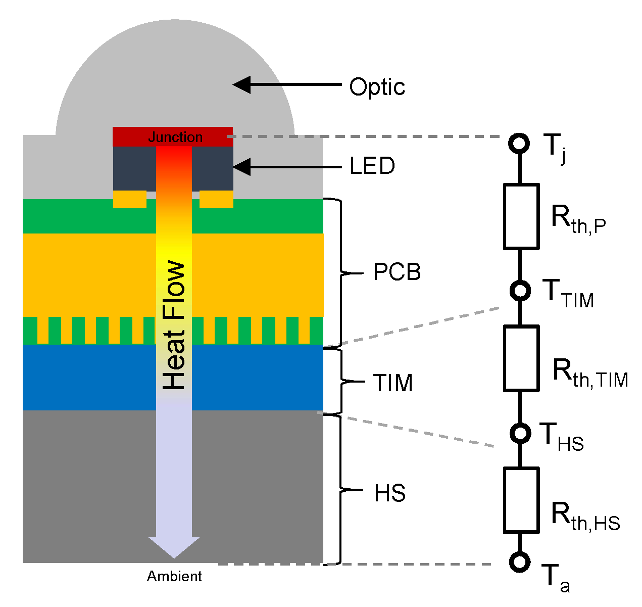
Figure 1. Structure of a typical LED system and its main thermal resistances determining the heat flow from junction to ambient.
Applsci 12 10063 g001
Figure 2. Schematic diagram of the LED electrical model.
Applsci 12 10063 g002
Figure 3. Workflow: (1) BHM framework (Section 3.2), (2) data-driven model for LED degradation [43], (3) impact of uncertainty in Δ T 0 on RUL prediction (Section 6.2).
Applsci 12 10063 g003
Figure 4. Representation of the BHM in (11) as a directed acyclic graph (DAG).
Applsci 12 10063 g004
Figure 5. MCMC diagnostics for σ R th for a single dataset of E1 ( n 2 = 100 , Issue 1): (left) trace plot with true values (red dashed line) and burn-in phase (gray line); (right) ACF plot after thinning and the burn-in phase.
Applsci 12 10063 g005
Figure 6. Posterior marginals of (left) μ R th and (right) σ R th for a single dataset of E1 ( n 2 = 100 , Issue 1) with 95%-HPD regions, true values (red circle) and (uniform) prior distributions (yellow line).
Applsci 12 10063 g006
Figure 7. Visualization of Table 1: Distribution of posterior means for μ R th (left) and σ R th (right) over 100 datasets (E1) for different sample sizes ( n 1 = 20 , n 2 = 100 and n 3 = 500 ), true values (red circle) and (uniform) prior distributions (yellow line).
Applsci 12 10063 g007
Figure 8. (Left) Posterior marginal of the thermal resistance R th for a single dataset of E1 ( n 2 = 100 , Issue 1); (right) posterior predictive distribution for the respective dataset with posterior mean (dashed line) and 95%-HPD region (arrows) of Δ T 0 and true value (red circle).
Applsci 12 10063 g008
Figure 9. Posterior distribution of σ ε for a single dataset of E2 (Issue 2) with 95%-HPD regions, true value (red circle) and prior distribution p ( σ ε ) B ( a 0 , b 0 ) (yellow line). (Left) n 2 = 100 and a 0 = b 0 = 12 ; (right) n 3 = 500 and a 0 = b 0 = 40 .
Applsci 12 10063 g009
Figure 10. Visualization of Table 2: Distribution of posterior means for (left) μ R th and (right) σ R th over 100 datasets (E3.a–E3.c) under different strategies, true values (red circle) and (uniform) prior distributions (yellow line).
Applsci 12 10063 g010
Figure 11. Reliability workflow of the dataset [52] using thermo–electrical loading conditions as input parameters to age the LED system. Thermal impedance (TI) analysis is further used for intake and a sequential analytical method to evaluate the status of the device under test (DuT).
Applsci 12 10063 g011
Figure 12. Bayesian RUL prediction of LED systems as proposed in [43]: Measured data (red circles) with error bars representing the measurement uncertainty obtained from 20 repeated measurements on a single LED device under constant conditions, i.e., ±2 σ ˜ with σ ˜ ≈ 0.5 °C; estimated values (green circles); and predictions of Δ T j (green dashed line). Probability density function (pdf) of failure based on a failure threshold used to indicate end-of-life.
Applsci 12 10063 g012
Figure 13. Impact of uncertainty in the initial temperature swing on RUL prediction in the presence of production and application variability: σ R th = 1 K/W (left), σ R th = 0.3 K/W (right). Results: (a) pdf of failure based on failure threshold, (b) model predictions with 95% credible intervals based on the predictive uncertainty in Δ T 0 from Section 5.1 (E1).
Applsci 12 10063 g013
Table 1. Simulation results for Issue 1 (I1, Section 4.2) and Issue 2 (I2, Section 4.3). Averaged posterior means (Av. post. mean) for μ R th , σ R th and σ ε (only I2); averaged lower and upper bounds of 95%-HPD regions (Av. 95%-HPD) for μ R th , σ R th and σ ε (only I2); and respective length of averaged 95%-HPD regions (Length HPD) over 100 datasets based on different sample sizes ( n 1 = 20 , n 2 = 100 and n 3 = 500 ).
IssueParameterTruenAv. Post.Av. 95%-Length
Value MeanHPDHPD
(I1) Production & application μ R th 39.13  2039.133[38.662,39.609]0.948
        variability 10039.133[38.931,39.335]0.404
50039.128[39.009,39.254]0.246
σ R th    1.00  20  1.042[0.710,1.426]0.716
100  1.015[0.872,1.165]0.293
500  1.007[0.937,1.095]0.158
(I2) Measurement μ R th 39.13  2039.133[38.659,39.609]0.950
       uncertainty 10039.133[38.931,39.335]0.404
50039.128[39.039,39.217]0.178
σ R th    1.00  20  1.042[0.709,1.426]0.717
100  1.014[0.871,1.165]0.294
500  1.003[0.939,1.068]0.129
σ ε    0.50  20  0.501[0.307,0.694]0.387
100  0.502[0.312,0.687]0.375
500  0.497[0.402,0.595]0.193
Table 2. Simulation results for Issue 3 (I3, Section 4.4) based on experiments E3.a–E3.c. Averaged posterior means (Av. post. mean) for μ R th and σ R th , averaged lower and upper bounds of 95%-HPD regions (Av. 95%-HPD) for μ R th and σ R th , and respective length of the averaged 95%-HPD regions (Length HPD) over 100 datasets based on n = 100 observations.
IssueParameterTrueStrategyAv. Post.Av. 95%-Length
Value MeanHPDHPD
(I3) Uncertain experimental μ R th 39.131. idealized39.130[38.930,39.332]0.402
       conditions 2. ignorant39.134[38.696,39.574]0.878
3. proper39.134[38.745,39.541]0.796
σ R th   1.001. idealized  1.011[0.869,1.162]0.293
2. ignorant  2.231[1.924,2.558]0.633
3. proper  1.051[0.614,1.502]0.888
Publisher’s Note: MDPI stays neutral with regard to jurisdictional claims in published maps and institutional affiliations.