

Bio-Inspired Model-Based Design and Control of Bipedal Robot


Abstract
1. Introduction
2. Analysis of the Problem Area
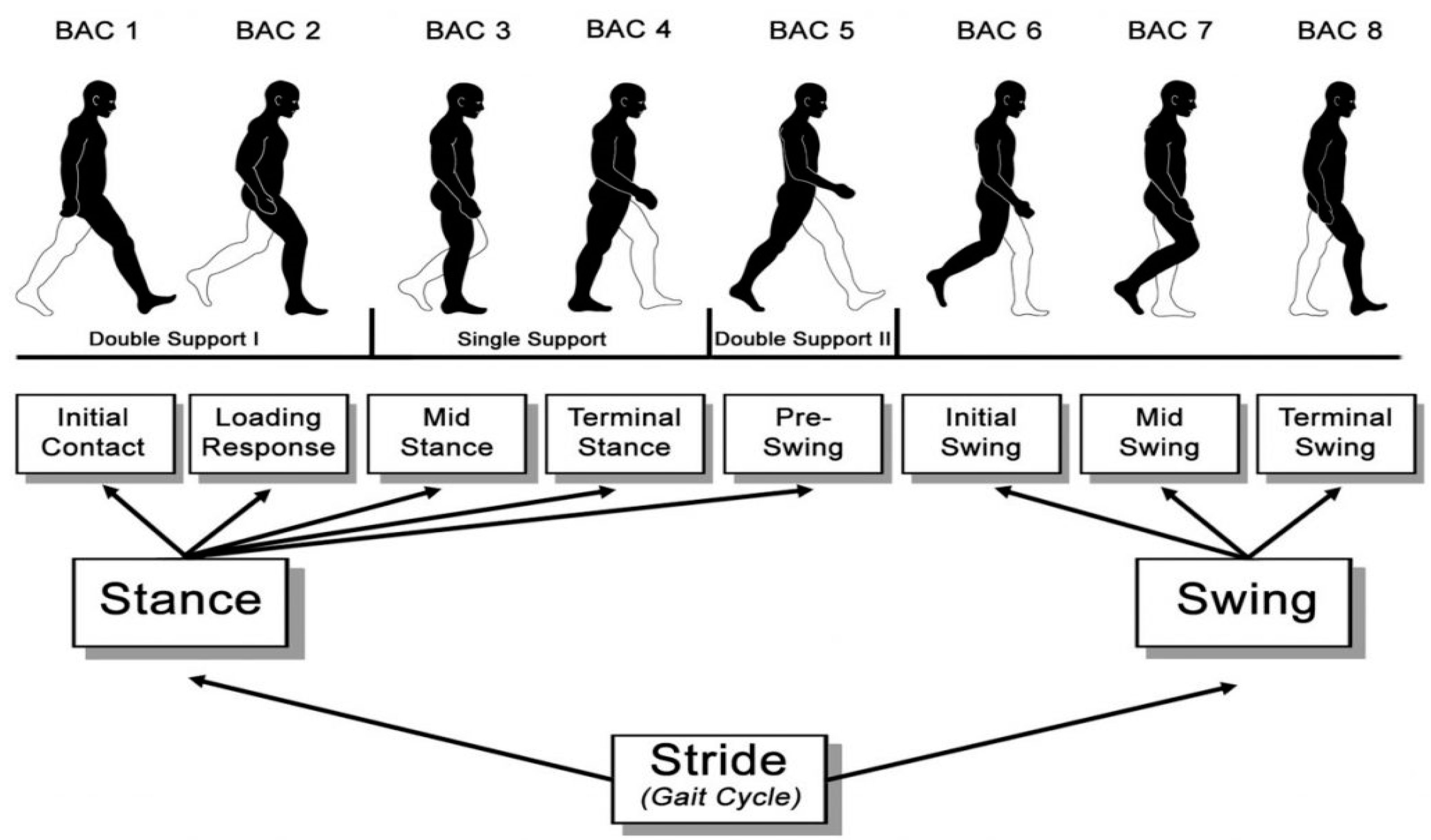
2.1. Dynamic Side of the Problem—Human Walking
- Lifting the heel off the ground while keeping the toe in contact with the ground. This action is included in the BAC 5 phase. It forms the transition between the one-limbed stance and the swing itself [5].
- The movement (swaying) of the leg in front of the person’s gravity center is described in the events of BAC 6 and BAC 7. The distance that the leg travels from the beginning of the BAC 6 phase to the end of BAC 7 is defined as the step length [5].
2.2. Static Side of the Problem—Construction Solution
- the ratio of the dimensions of the frame and individual arms, including the joints of the robot, was as similar as possible to the ratio of the dimensions of human limbs,
- the center of gravity of the robot was placed as close as possible to the position of the human body.
3. Modeling and Simulation of Biped Robot
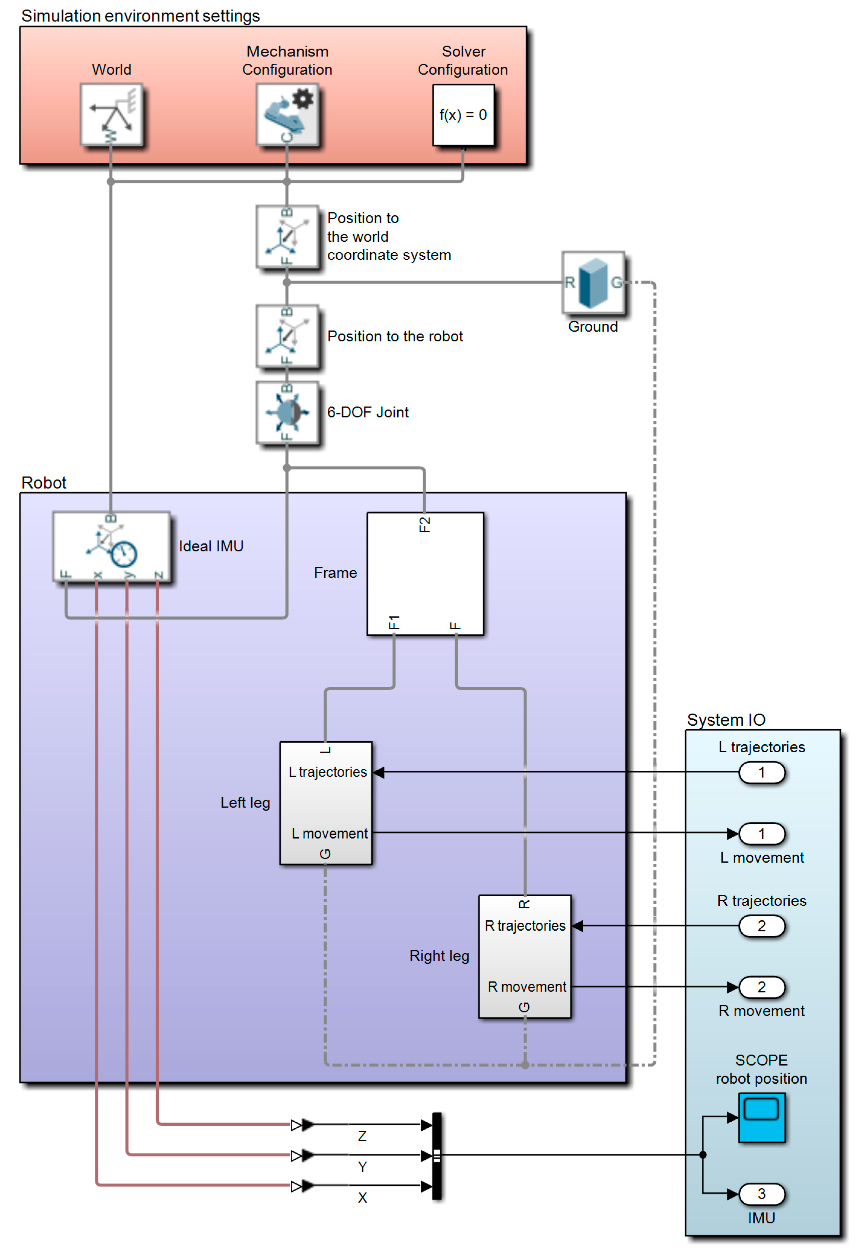
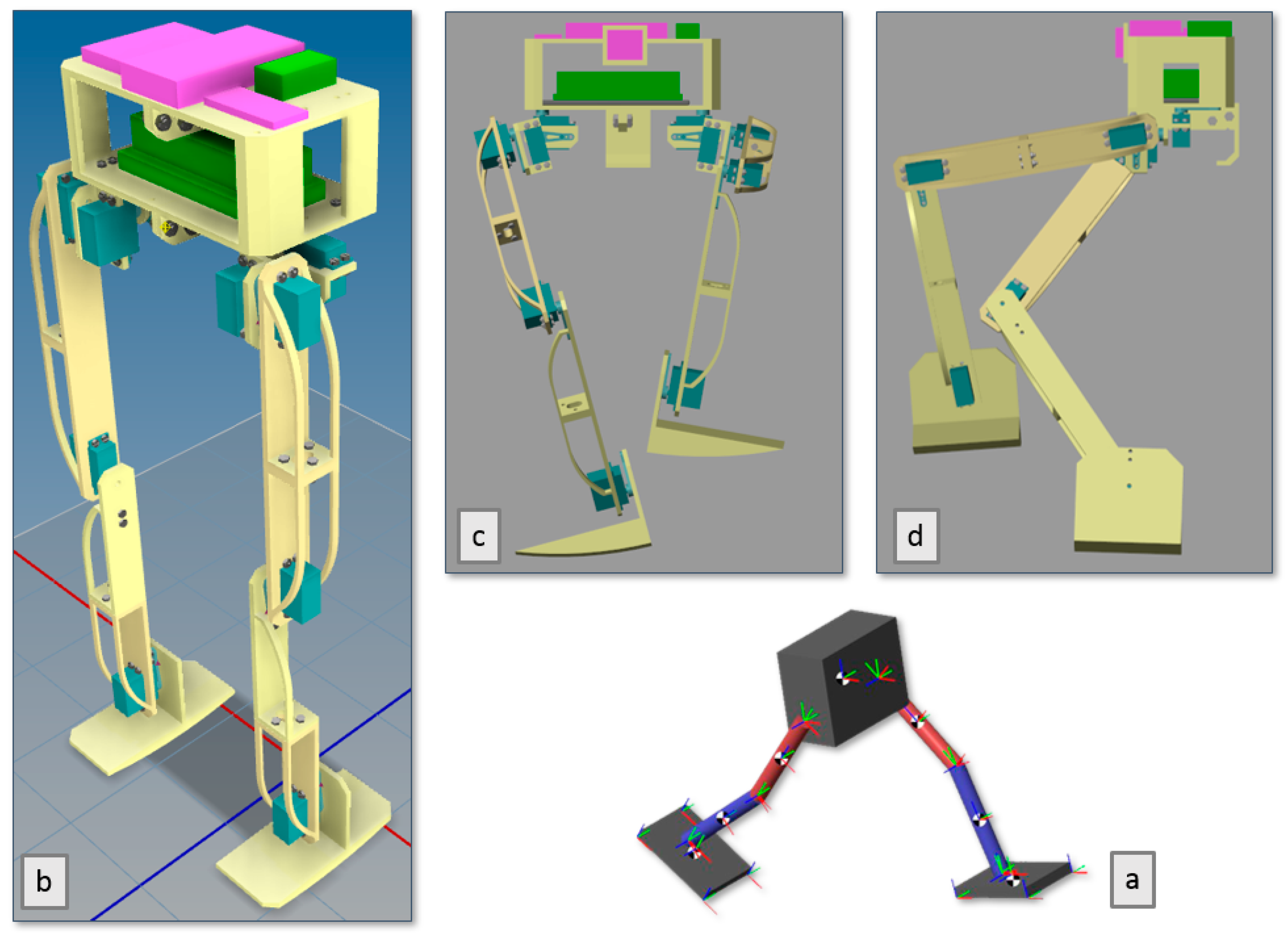
3.1. Design of a Simulation Model of a Bipedal Robot
- The frame is a mobile base on which two manipulators are attached. The center of gravity of the robot is also located in this part and forms the material part (the head) of the inverse pendulum. The frame represents the human pelvis.
- The left leg is the manipulator of the robot, one end of which is attached to the left side of the frame, and the other end is terminated by an effector. The manipulator consists of four arms and six joints. The manipulator represents the arm of the inverted pendulum and the human leg, where the effector fulfills the role of the foot.
- The right leg is a manipulator functionally identical to the left leg, but it is fixed on the right side of the frame.
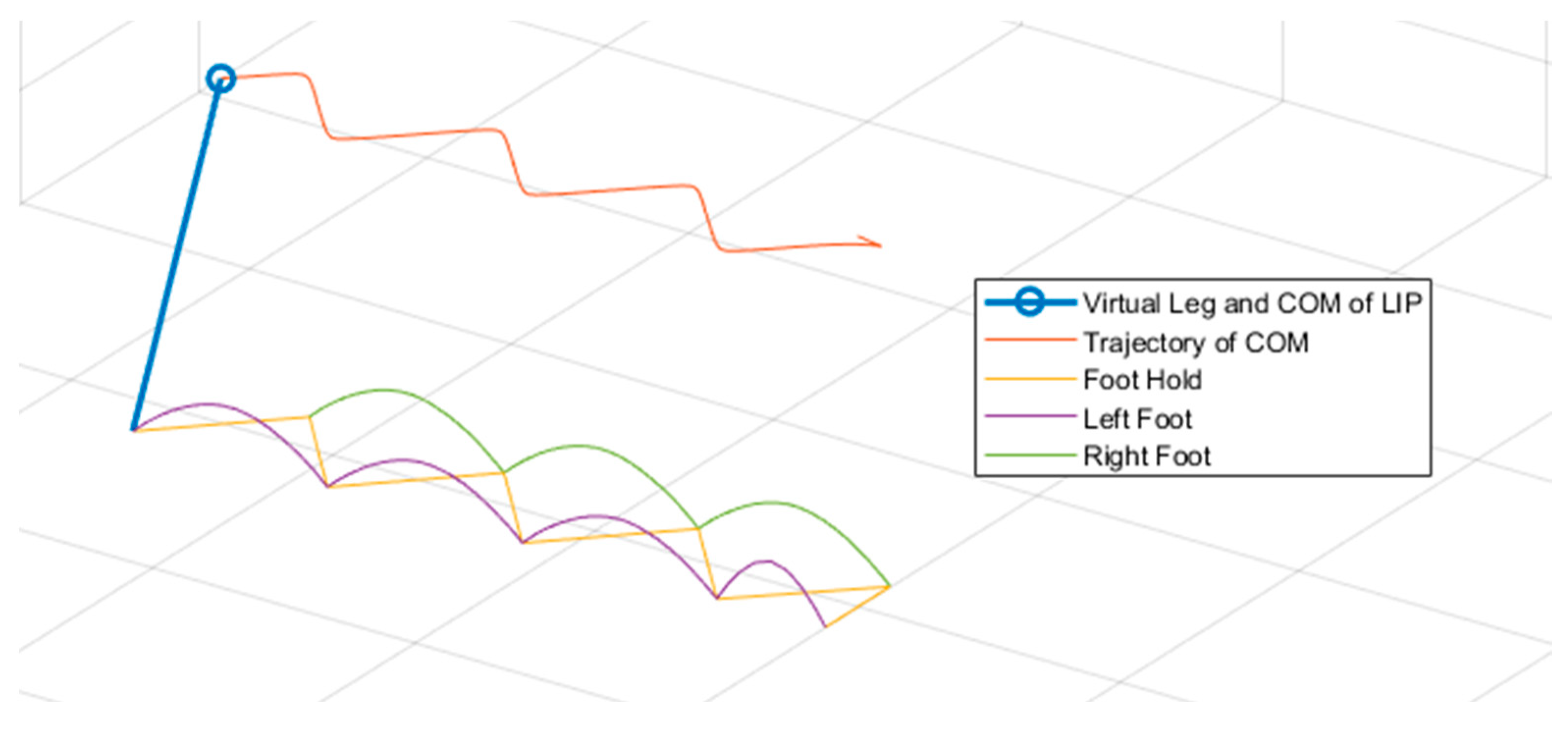
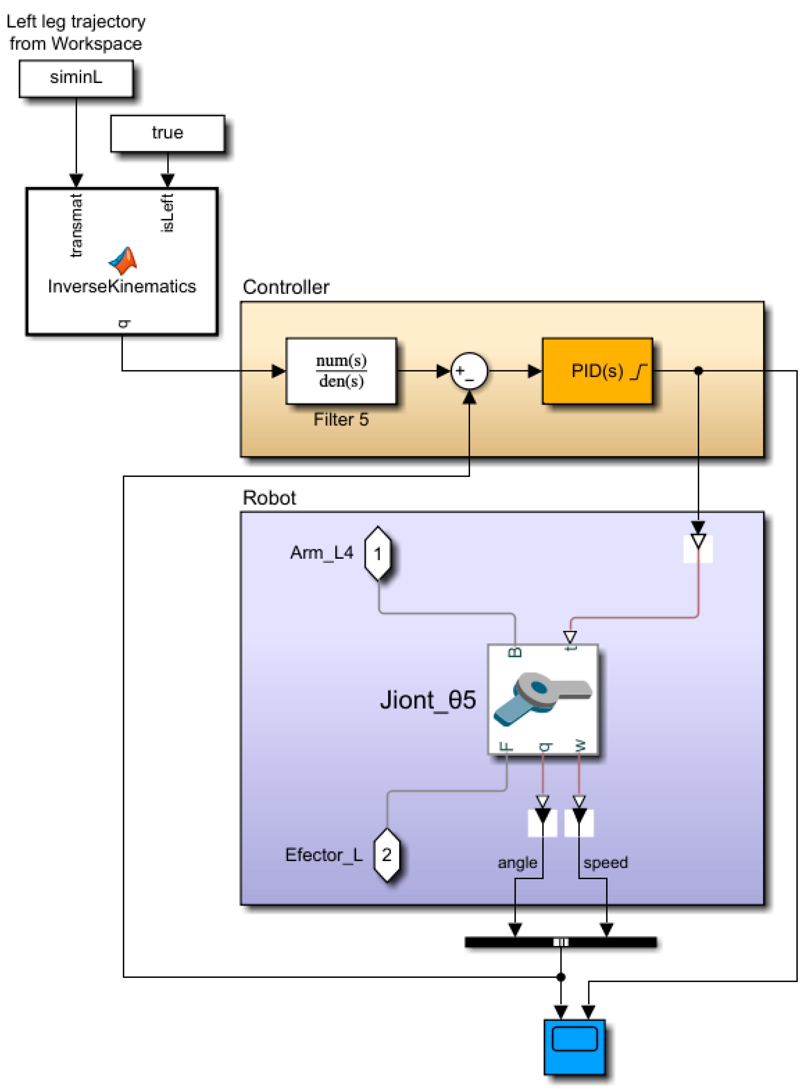
3.2. Simulation of a Bipedal Robot Walking
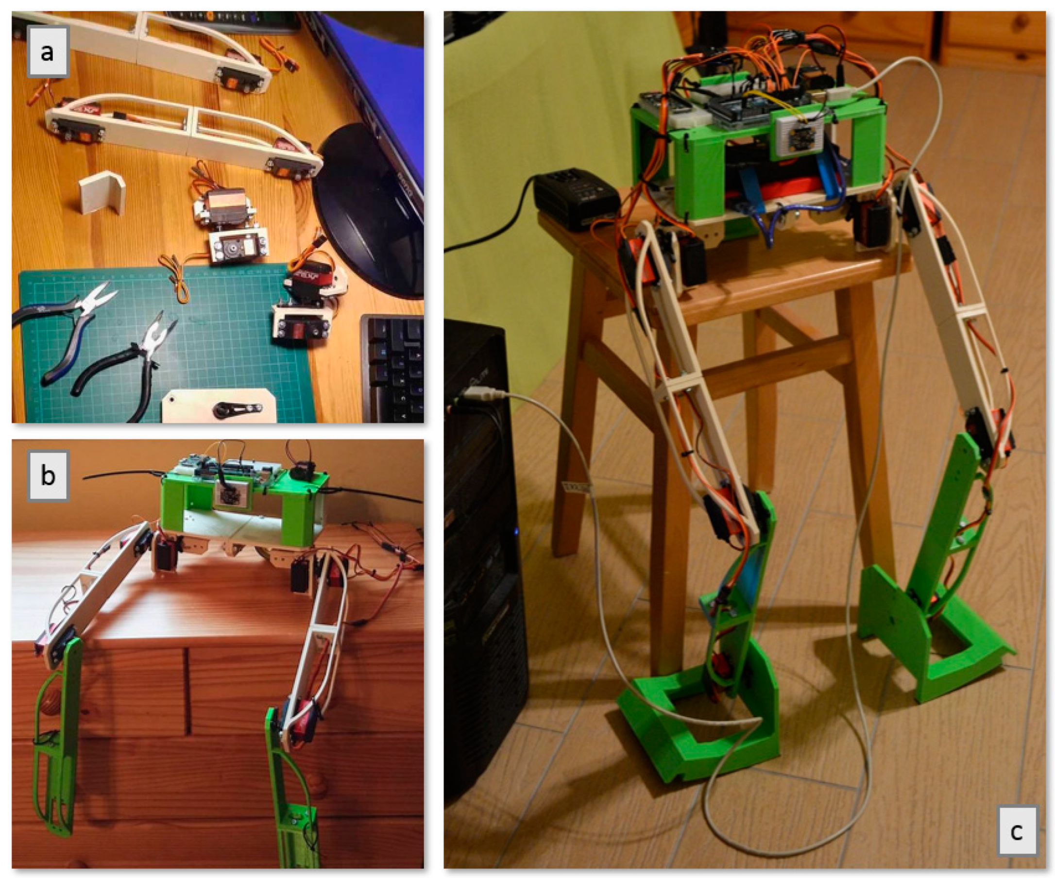
4. Realization of a Physical Model of a Bipedal Robot
4.1. Construction of a Bipedal Robot
4.2. Control Hardware
5. Solution Testing and Discussion
6. Conclusions
Author Contributions
Funding
Conflicts of Interest
References
- Boston Dynamics. ATLASTM. Available online: https://www.bostondynamics.com/atlas (accessed on 1 April 2022).
- IEEE. Robots—Your Guide to the World of Robotics. Available online: https://robots.ieee.org/robots/digit (accessed on 1 April 2022).
- Yang, X.; She, H.; Lu, H.; Fukuda, T.; Shen, Y. State of the Art: Bipedal Robots for Lower Limb Rehabilitation. Appl. Sci. 2017, 7, 1182. [Google Scholar] [CrossRef]
- Gulletta, G.; Erlhagen, W.; Bicho, E. Human-Like Arm Motion Generation: A Review. Robotics 2020, 9, 102. [Google Scholar] [CrossRef]
- Perry, J.; Burnfield, J.M. Gait Analysis: Normal and Pathological Function; Slack Incorporated: West Deptford, NJ, USA, 2010; p. 551. ISBN 978-1556427664. [Google Scholar]
- Čapek, L.; Hájek, P.; Henyš, P. Biomechanika Člověka; Grada Publishing: Prague, Czech Republic, 2018; ISBN 978-80-271-0367-6. [Google Scholar]
- Stöckel, T.; Jacksteit, R.; Behrens, M.; Skripitz, R.; Bader, R.; Mau-Moeller, A. The Mental Representation of the Human Gait in Young and Older Adults. Front. Psychol. 2015, 6, 943. [Google Scholar] [CrossRef]
- Mitobe, K.; Capi, G.; Takayama, H.; Yamano, M.; Nasu, Y. A ZMP Analysis of the Passive Walking Machines. In Proceedings of the SICE 2003 Annual Conference (IEEE Cat. No.03TH8734), Fukui, Japan, 4–6 August 2003; Volume 1, pp. 112–116. [Google Scholar]
- Omer, A.; Hashimoto, K.; Lim, H.-O.; Takanishi, A. Study of Bipedal Robot Walking Motion in Low Gravity: Investigation and Analysis. Int. J. Adv. Robot. Syst. 2014, 11, 139. [Google Scholar] [CrossRef]
- Lanari, L.; Hutchinson, S.; Marchionni, L. Boundedness Issues in Planning of Locomotion Trajectories for Biped Robots. In Proceedings of the 2014 IEEE-RAS International Conference on Humanoid Robots, Atlanta, GA, USA, 18–20 November 2014; pp. 951–958. [Google Scholar]
- Bakaráč, P. Konštrukcia a Riadenie Inverzného Kyvadla. Master’s Thesis, Slovak University of Technology in Bratislava, Bratislava, Slovakia, 2017. [Google Scholar]
- Erbatur, K.; Kurt, O. Natural ZMP Trajectories for Biped Robot Reference Generation. IEEE Trans. Ind. Electron. 2009, 56, 835–845. [Google Scholar] [CrossRef]
- Prokopenko, S. Human Figure Proportions—Cranial Units—Robert Beverly Hale. Available online: https://www.proko.com/human-figure-proportions-cranium-unit-hale (accessed on 1 April 2022).
- Vachálek, J.; Takács, G. Robotika; STU Publishing: Bratislava, Slovakia, 2014; p. 166. ISBN 978-80-227-4163-7. [Google Scholar]
- Somisetti, K.; Tripathi, K.; Verma, J.K. Design, Implementation, and Controlling of a Humanoid Robot. In Proceedings of the 2020 International Conference on Computational Performance Evaluation (ComPE), Shillong, India, 2–4 July 2020; pp. 831–836. [Google Scholar]
- Hamilton, N.; Weimar, W.; Luttgens, K. Kinesiology: Scientific Basis of Human Motion, 12th ed.; McGraw Hill: New York, NY, USA, 2012; p. 640. ISBN 978-0078022548. [Google Scholar]
- McGeer, T. Passive Dynamic Walking. Int. J. Robot. Res. 1990, 9, 62–82. [Google Scholar] [CrossRef]
- Yamane, K.; Trutoiu, L. Effect of Foot Shape on Locomotion of Active Biped Robots. In Proceedings of the 2009 9th IEEE-RAS International Conference on Humanoid Robots, Paris, France, 7–10 December 2009; pp. 230–236. [Google Scholar]
- Virgala, I.; Miková, Ľ.; Kelemenová, T.; Varga, M.; Rákay, R.; Vagaš, M.; Semjon, J.; Jánoš, R.; Sukop, M.; Marcinko, P.; et al. A Non-Anthropomorphic Bipedal Walking Robot with a Vertically Stabilized Base. Appl. Sci. 2022, 12, 4108. [Google Scholar] [CrossRef]
- Che, J.; Pan, Y.; Yan, W.; Yu, J. Leg Configuration Analysis and Prototype Design of Biped Robot Based on Spring Mass Model. Actuators 2022, 11, 75. [Google Scholar] [CrossRef]
- Babinec, A. Riadenie Robotických Manipulátorov. Lectures; Faculty of Electrical Engineering and Information Technology STU: Bratislava, Slovakia, 2019. [Google Scholar]
- Kajita, S.; Kanehiro, F.; Kaneko, K.; Yokoi, K.; Hirukawa, H. The 3D Linear Inverted Pendulum Mode: A Simple Modeling for a Biped Walking Pattern Generation. In Proceedings of the 2001 IEEE/RSJ International Conference on Intelligent Robots and Systems. Expanding the Societal Role of Robotics in the the Next Millennium (Cat. No.01CH37180), Maui, HI, USA, 29 October–3 November 2001; Volume 1, pp. 239–246. [Google Scholar]
- Robotshop. Arduino Mega 2560 Datasheet. Available online: https://www.robotshop.com/media/files/pdf/arduinomega2560datasheet.pdf (accessed on 1 April 2022).
- Raspberry Pi Foundation. Raspberry Pi Hardware. Available online: https://www.raspberrypi.org/documentation/hardware/raspberrypi (accessed on 1 April 2022).
- Adafruit. Adafruit BNO055 Absolute Orientation Sensor. Available online: https://learn.adafruit.com/adafruit-bno055-absolute-orientation-sensor (accessed on 1 April 2022).


| Point 1 | Point 2 | Number of Units |
|---|---|---|
| right hip joint | left hip joint | 2 |
| hip joint | knee | 3 |
| knee | ground (bottom of heel) | 3 |
| Coupling | DOF | Type of Kinematic Pair |
|---|---|---|
| hip joint | 3 | spherical |
| knee | 1 | rotary |
| ankle | 2 | two cylindrical |
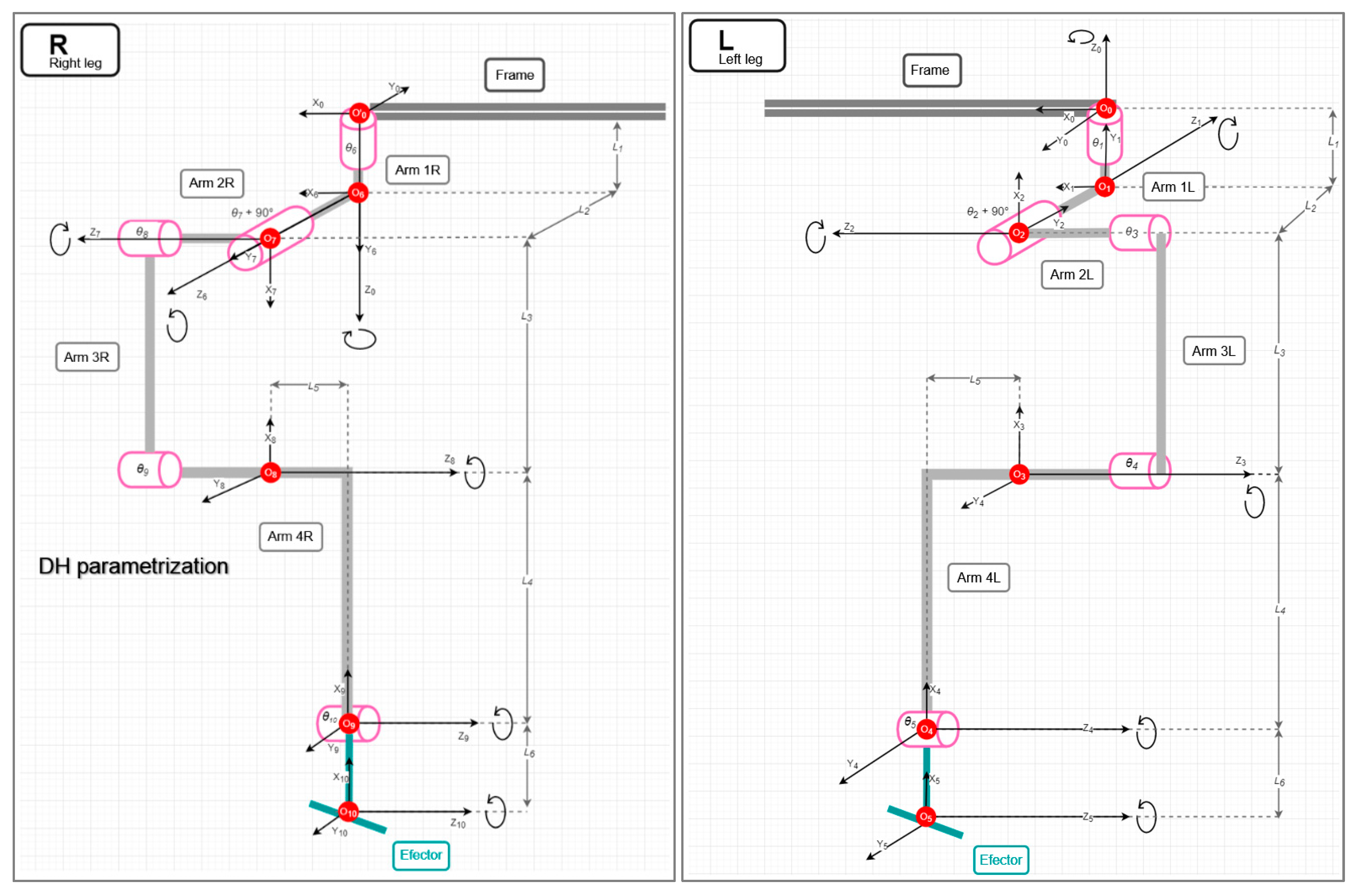
| Left ai [mm] 1 | αi [deg] 2 | di [mm] 3 | θi [deg] 4 |
|---|---|---|---|
| 0 | 90 | L1 | θ1 |
| 0 | −90 | L2 | θ2 + 90 |
| L3 | 180 | 0 | θ3 |
| L4 | 0 | L5 | θ4 |
| L6 | 0 | 0 | θ5 |
| Right ai [mm] 1 | αi[deg] 2 | di [mm] 3 | θi[deg] 4 |
| 0 | 90 | L1 | θ6 |
| 0 | 90 | L2 | θ7—90 |
| L3 | 180 | 0 | θ8 |
| L4 | 0 | L5 | θ9 |
| L6 | 0 | 0 | θ10 |
| Property | Value | Unit |
|---|---|---|
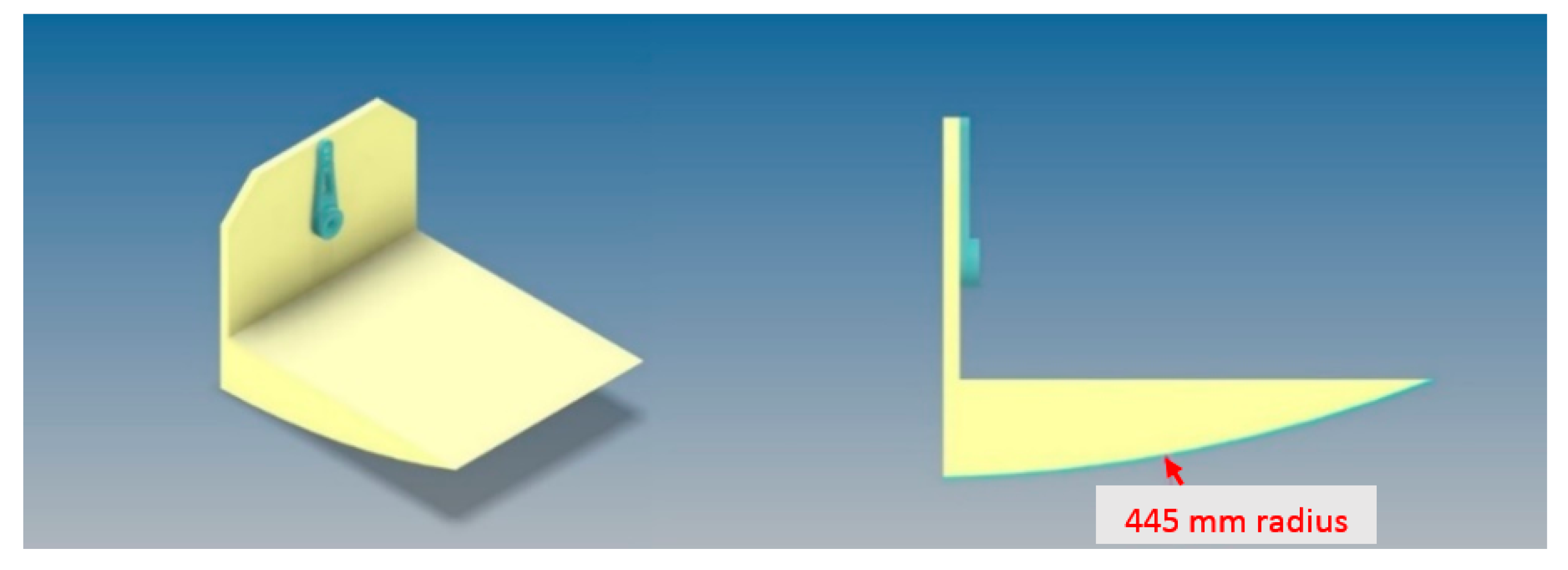
| the height of the robot’s center of gravity | 445 | mm |
| height of the center of gravity of the frame | 645 | mm |
| foot height | 30 | mm |
| the length of the foot arch | 144 | mm |
| the weight of the robot | 2.755 | kg |
| Parameter | Model | Value | Unit |
|---|---|---|---|
| spread of the legs in the starting position | Lr + L5 | 0.091 | m |
| height of the frame in the starting position | h | 0.644 | m |
| frame height while walking | hw | 0.570 | m |
| spread of the legs during gait | La | 0.144 | m |
| step length in walking direction | Ls | 0.020 | m |
| Test No. | Property [Unit] | Value (Physical Model) | Value (Simulation Model) | Deviation |
|---|---|---|---|---|
| 1 | weight [kg] | 3.06 | 2.75 | 0.31 |
| 2 | length L1 [mm] | 16 | 31 | 15 |
| 3 | length L2 [mm] | 29 | 51 | 22 |
| 4 | length L3 [mm] | 254 | 252 | 2 |
| 5 | length L4 [mm] | 263 | 262 | 1 |
| 6 | length L5 [mm] | 18 | 27 | 9 |
| 7 | length L6 [mm] | 62 | 25 | 37 |
| 8 | step length in the starting position [mm] | 80 | 91 | 11 |
| 9 | frame height in the starting position [mm] | 599 | 570 (644) | 26 |
| Test No. | Step Length [mm] | Number of Successful Measurements | Number of Failed Measurements | The Largest Number of Steps Taken in a Failed Measurement (X/8) |
|---|---|---|---|---|
| 1 | 50 | 5 | 0 | - |
| 2 | 60 | 5 | 0 | - |
| 3 | 70 | 5 | 0 | - |
| 4 | 80 | 5 | 0 | - |
| 5 | 90 | 5 | 0 | - |
| 6 | 95 | 5 | 0 | - |
| 7 | 100 | 5 | 0 | - |
| 8 | 105 | 5 | 0 | - |
| 9 | 110 | 5 | 0 | - |
| 10 | 115 | 5 | 0 | - |
| 11 | 120 | 5 | 0 | - |
| 12 | 125 | 5 | 0 | - |
| 13 | 130 | 4 | 1 | 3 |
| 14 | 135 | 2 | 3 | 3 |
| 15 | 140 | 1 | 4 | 2 |
| 16 | 145 | 1 | 4 | 2 |
| 17 | 150 | 0 | 5 | 2 |
| 18 | 155 | 0 | 5 | 0 |
| - | - | ∑ = 90 | MAX = 3 |
Publisher’s Note: MDPI stays neutral with regard to jurisdictional claims in published maps and institutional affiliations. |
© 2022 by the authors. Licensee MDPI, Basel, Switzerland. This article is an open access article distributed under the terms and conditions of the Creative Commons Attribution (CC BY) license (https://creativecommons.org/licenses/by/4.0/).
Share and Cite
Polakovič, D.; Juhás, M.; Juhásová, B.; Červeňanská, Z. Bio-Inspired Model-Based Design and Control of Bipedal Robot. Appl. Sci. 2022, 12, 10058. https://doi.org/10.3390/app121910058
Polakovič D, Juhás M, Juhásová B, Červeňanská Z. Bio-Inspired Model-Based Design and Control of Bipedal Robot. Applied Sciences. 2022; 12(19):10058. https://doi.org/10.3390/app121910058
Chicago/Turabian StylePolakovič, David, Martin Juhás, Bohuslava Juhásová, and Zuzana Červeňanská. 2022. "Bio-Inspired Model-Based Design and Control of Bipedal Robot" Applied Sciences 12, no. 19: 10058. https://doi.org/10.3390/app121910058
APA StylePolakovič, D., Juhás, M., Juhásová, B., & Červeňanská, Z. (2022). Bio-Inspired Model-Based Design and Control of Bipedal Robot. Applied Sciences, 12(19), 10058. https://doi.org/10.3390/app121910058