
A Skeleton-Line-Based Graph Convolutional Neural Network for Areal Settlements’ Shape Classification


Abstract
1. Introduction
2. Methodology
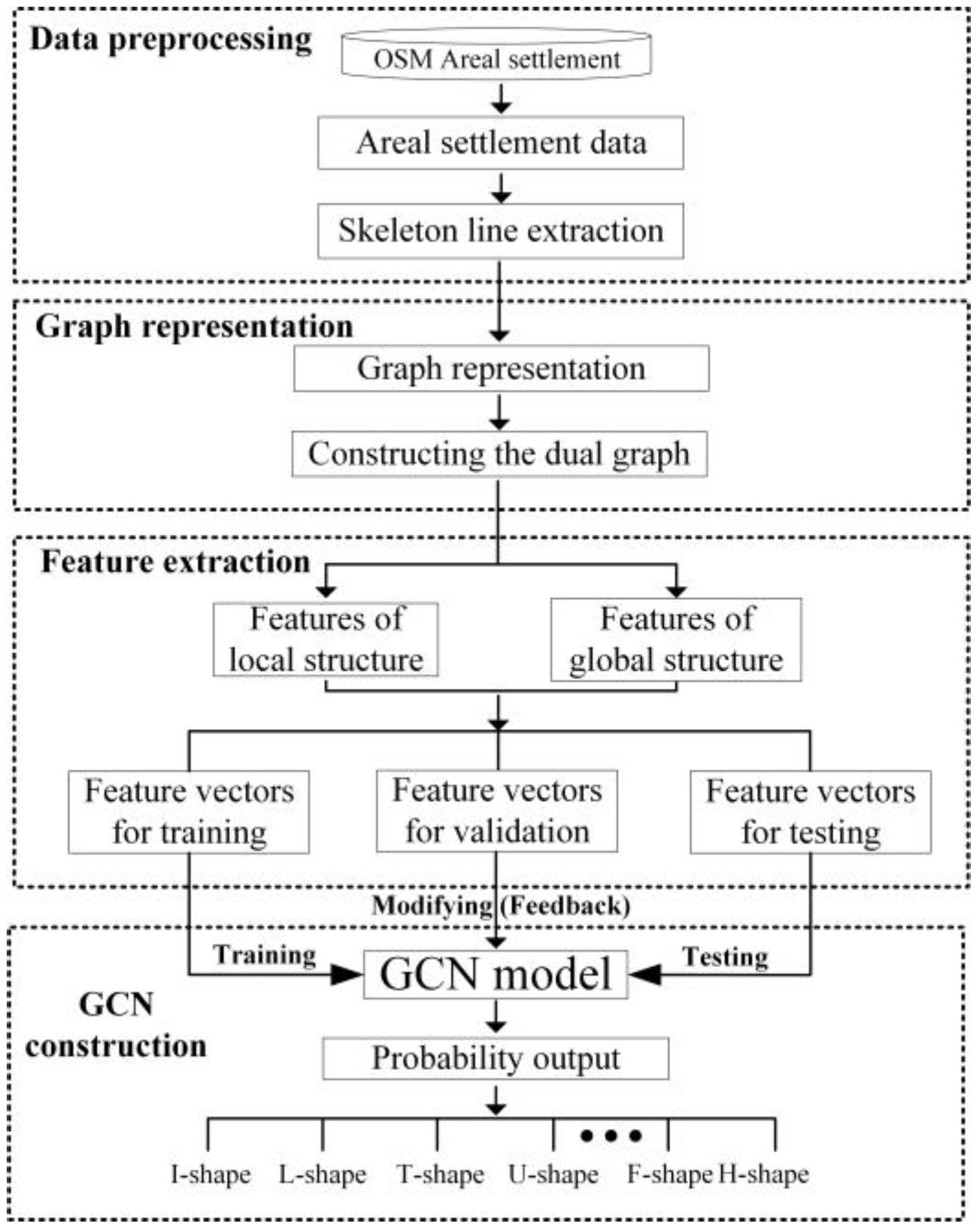
2.1. Framework
- (1)
- Data preprocessing: Areal settlement vector data were collected from the OSM dataset. Skeleton lines were constructed on the basis of the vector data of the areal settlement.
- (2)
- Graph representation: A component dual-graph structure was constructed on the basis of the skeleton line graph structure.
- (3)
- Feature extraction: Features of local and global structures representing the skeletal line dual graph of the areal settlement structure were extracted.
- (4)
- GCN construction: The model architecture based on the GCN was designed. Then, the GCN was trained and tested, Finally, a fully connected layer as a classifier completed the Areal settlements’ shape classification.
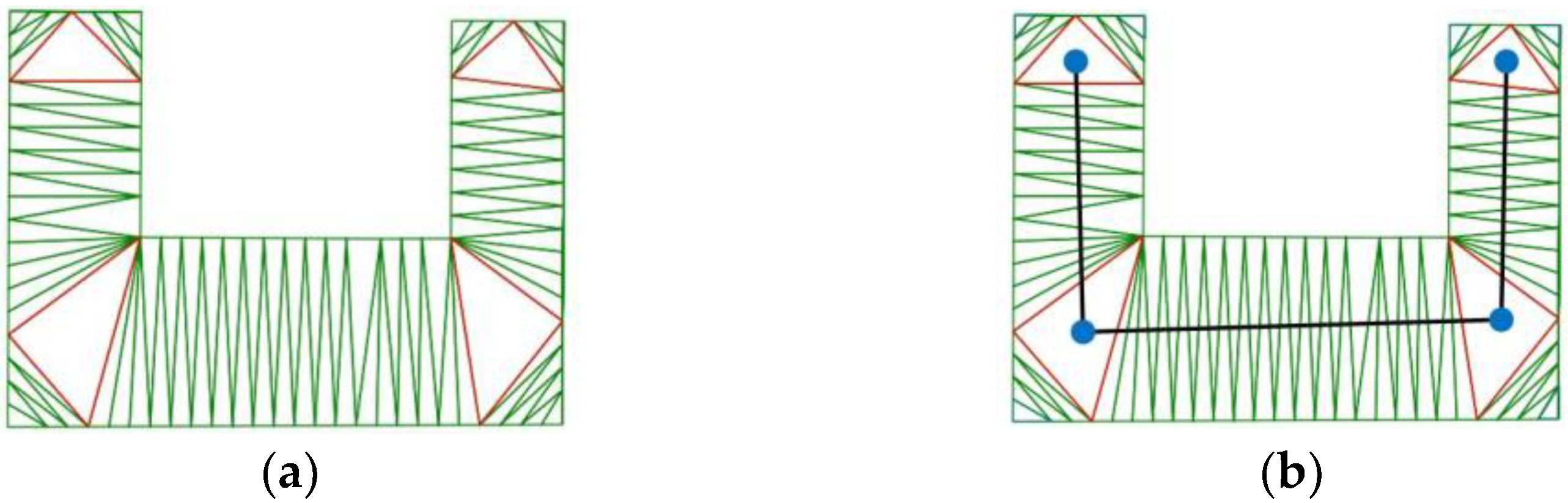
2.2. Data Preprocessing
2.3. Graph Representation
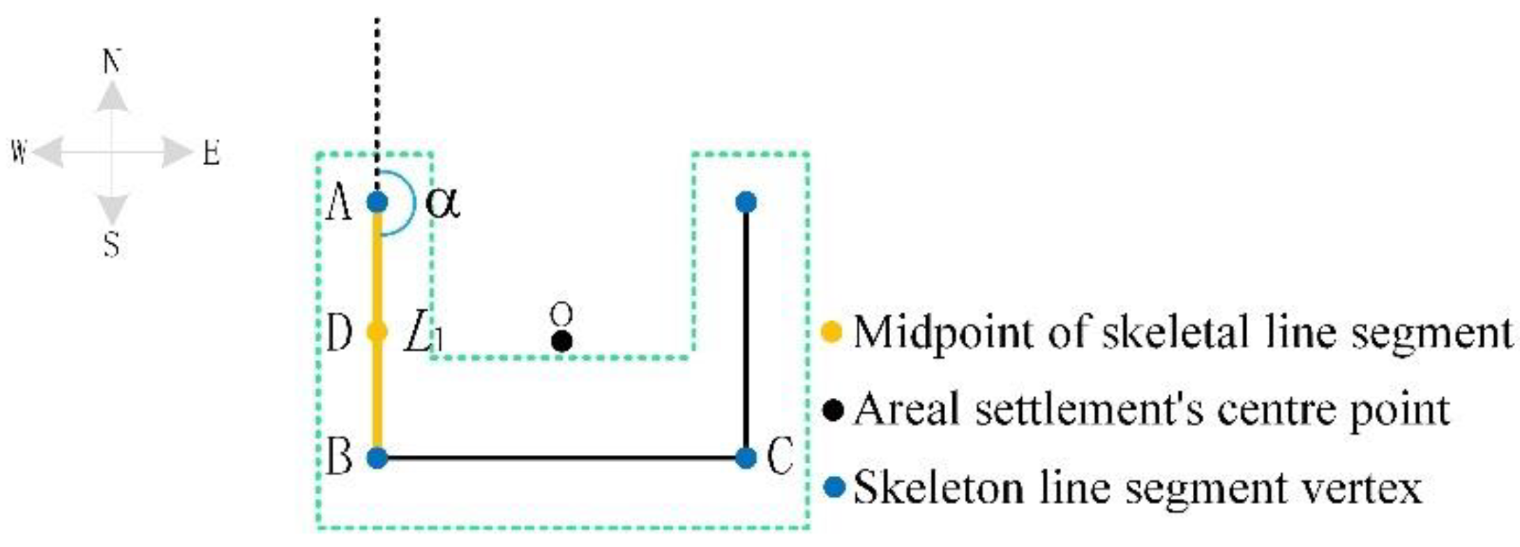
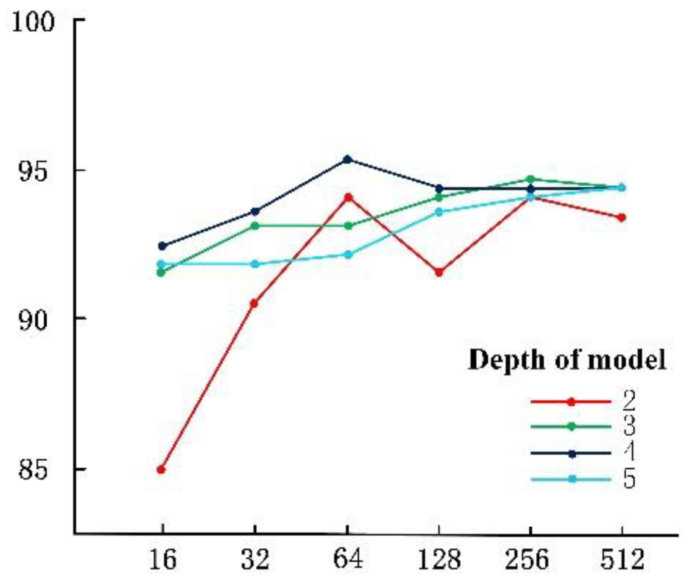
2.4. Feature Extraction
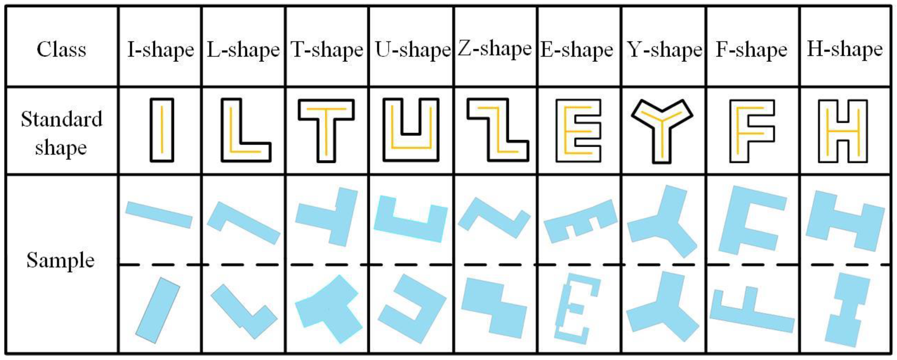
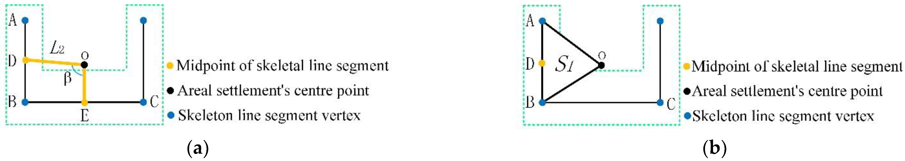
2.4.1. Local Features Extraction
2.4.2. Global Features Extraction
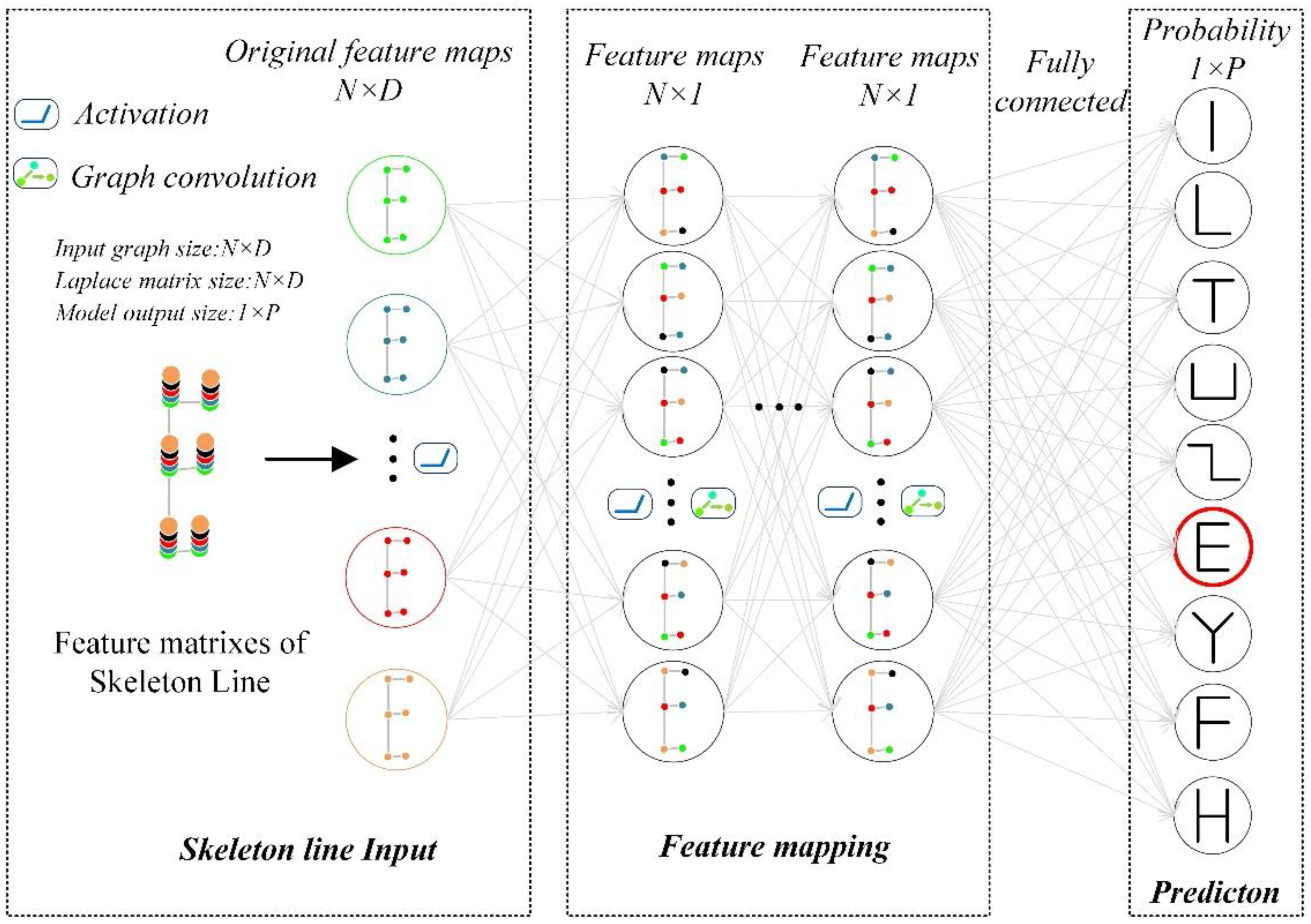
3. Structure of the GCN-Based Residential Classification Model
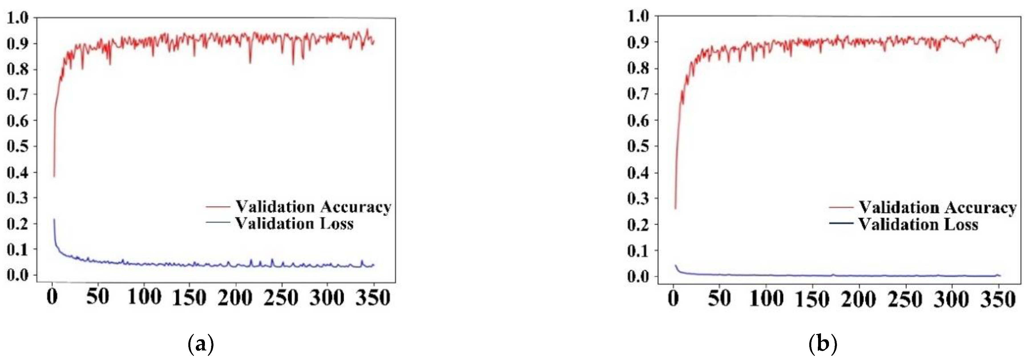
4. Experiments and Analysis
4.1. Experimental Environment and Data
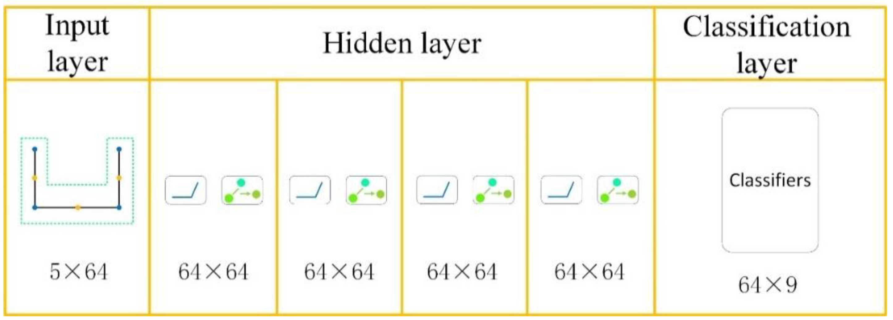
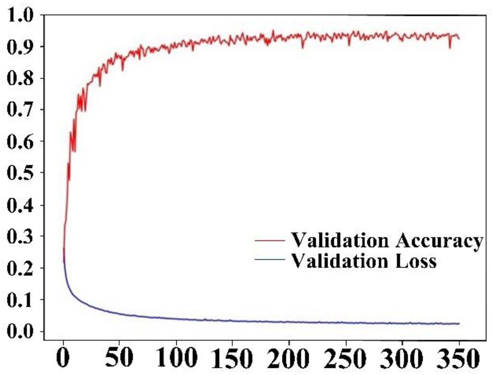
4.2. Model Structure and Parameter Settings
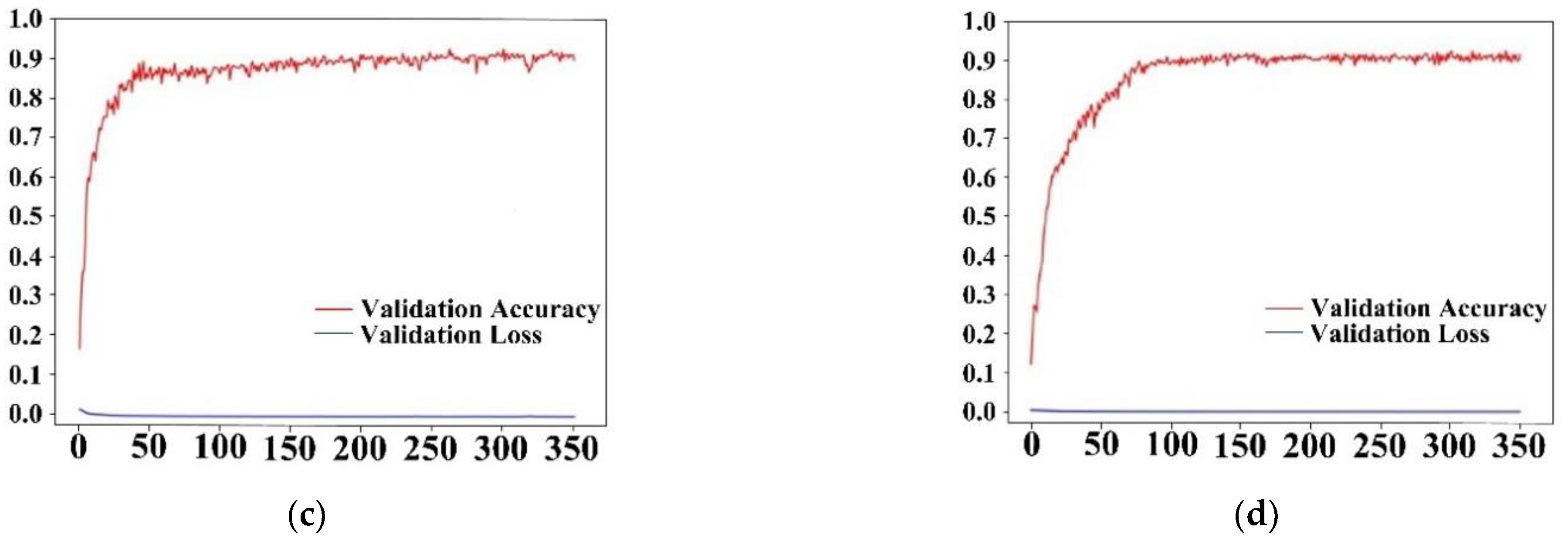
4.3. Sensitivity Analysis of Model Parameters
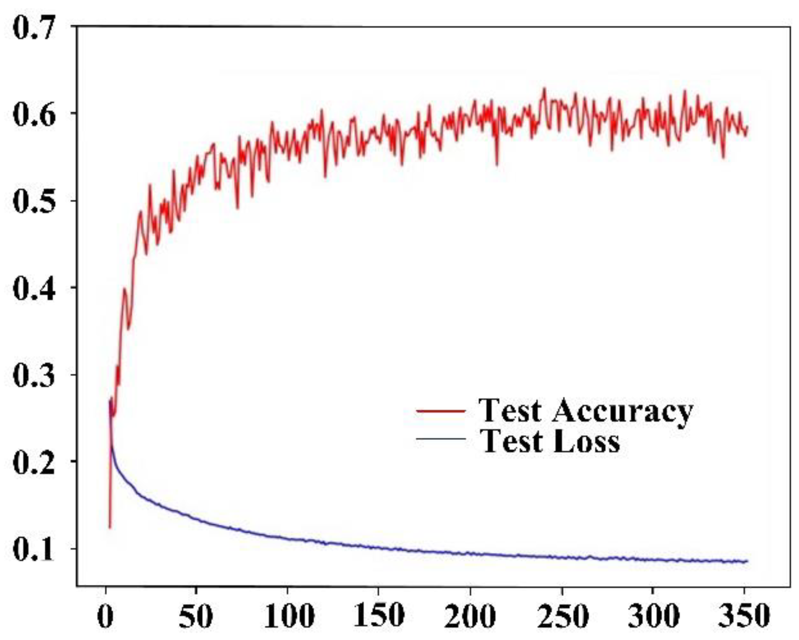
4.4. Classification Accuracy Analysis
4.5. Comparison to Other Methods
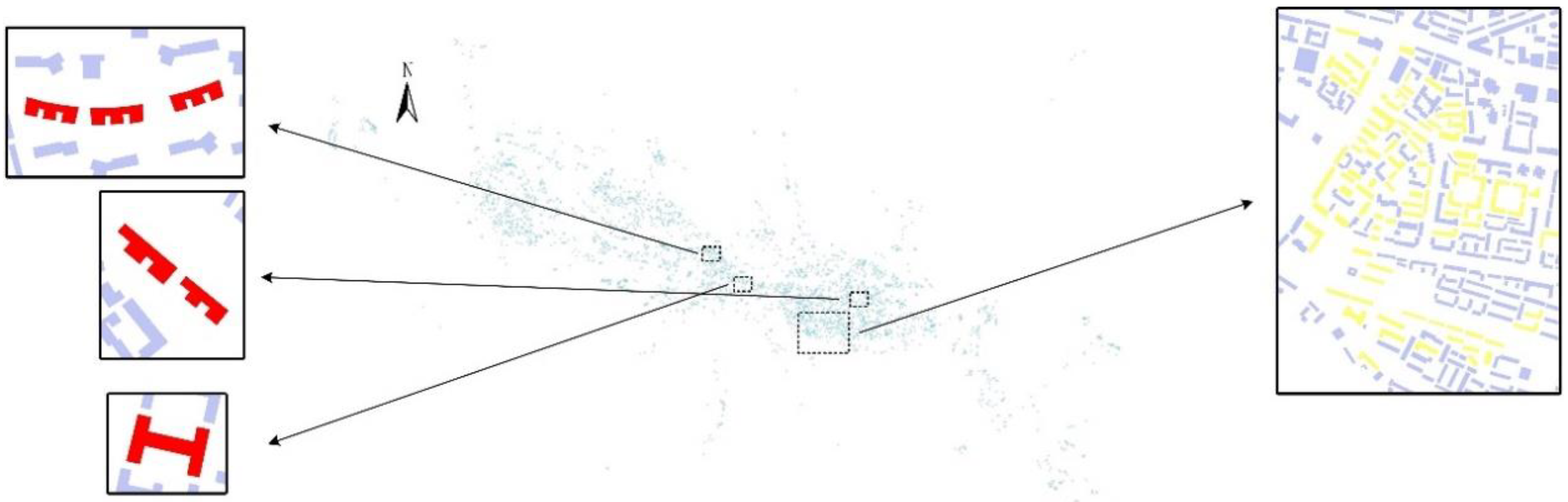
4.6. Applications
5. Conclusions
Author Contributions
Funding
Institutional Review Board Statement
Informed Consent Statement
Data Availability Statement
Conflicts of Interest
References
- Zhou, X.; Wang, H.; Wu, Z. An incremental updating method for land cover database using refined 2-dimensional intersection type. Acta Geod. Cartogr. Sin. 2017, 46, 114–122. [Google Scholar]
- Kim, J.-Y.; Yu, K.-Y. Automatic Detection of the Updating Object by Areal Feature Matching Based on Shape Similarity. J. Korean Soc. Surv. Geod. Photogramm. Cartogr. 2012, 30, 59–65. [Google Scholar] [CrossRef][Green Version]
- Zhang, X.; Stoter, J.; Ai, T. Automated evaluation of building alignments in generalized maps. Int. J. Geogr. Inf. Sci. 2013, 27, 1550–1571. [Google Scholar] [CrossRef]
- Stoter, J.; Burghardt, D.; Duchêne, C. Methodology for evaluating automated map generalization in commercial software. Comput. Environ. Urban Syst. 2009, 33, 311–324. [Google Scholar] [CrossRef]
- Harrie, L.; Stigmar, H.; Djordjevic, M. Analytical estimation of map readability. ISPRS Int. J. Geo-Inf. 2015, 4, 418–446. [Google Scholar] [CrossRef]
- Palmer, S.E. Vision Science: Photons to Phenomenology; MIT Press: Cambridge, MA, USA, 1999. [Google Scholar]
- Liu, Y.K.; Žalik, B. An efficient chain code with Huffman coding. Pattern Recognit. 2005, 38, 553–557. [Google Scholar]
- Belongie, S.; Malik, J.; Puzicha, J. Shape matching and object recognition using shape contexts. IEEE Trans. Pattern Anal. Mach. Intell. 2002, 24, 509–522. [Google Scholar] [CrossRef]
- Peter, A.M.; Rangarajan, A. Maximum likelihood wavelet density estimation with applications to image and shape matching. IEEE Trans. Image Process. 2008, 17, 458–468. [Google Scholar] [CrossRef]
- Saavedra, J.M. Sketch based image retrieval using a soft computation of the histogram of edge local orientations (s-helo). In Proceedings of the 2014 IEEE International Conference on Image Processing (ICIP), Paris, France, 27–30 October 2014; pp. 2998–3002. [Google Scholar]
- Yan, X.; Ai, T.; Yang, M. A Simplification of Residential Feature by the Shape Cognition and Template Matching Method. Acta Geod. Cartogr. Sin. 2016, 45, 874–882. [Google Scholar] [CrossRef]
- Ai, T.; Cheng, X.; Liu, P.; Yang, M. A shape analysis and template matching of building features by the Fourier transform method. Comput. Environ. Urban Syst. 2013, 41, 219–233. [Google Scholar] [CrossRef]
- Alajlan, N.; El Rube, I.; Kamel, M.S.; Freeman, G. Shape retrieval using triangle-area representation and dynamic space warping. Pattern Recognit. 2007, 40, 1911–1920. [Google Scholar] [CrossRef]
- Yang, C.; Wei, H.; Yu, Q. A novel method for 2D nonrigid partial shape matching. Neurocomputing 2018, 275, 1160–1176. [Google Scholar] [CrossRef]
- Cheng, M.; Sun, Q.; Xu, L.; Cheng, H. Polygon contour similarity and complexity measurement and application in simplification. Acta Geod. Cartogr. Sin. 2019, 48, 489–501. [Google Scholar] [CrossRef]
- Mokhtarian, F.; Mackworth, A.K. A theory of multiscale, curvature-based shape representation for planar curves. IEEE Trans. Pattern Anal. Mach. Intell. 1992, 14, 789–805. [Google Scholar] [CrossRef]
- Arkin, E.M.; Chew, L.P.; Huttenlocher, D.P.; Kedem, K.; Mitchell, J.S. An Efficiently Computable Metric for Comparing Polygonal Shapes; Cornell University: Ithaca, NY, USA, 1991. [Google Scholar]
- Basaraner, M.; Cetinkaya, S. Performance of shape indices and classification schemes for characterising perceptual shape complexity of building footprints in GIS. Int. J. Geogr. Inf. Sci. 2017, 31, 1952–1977. [Google Scholar] [CrossRef]
- Krizhevsky, A.; Sutskever, I.; Hinton, G.E. Imagenet classification with deep convolutional neural networks. Adv. Neural Inf. Process. Syst. 2012, 25, 84–90. [Google Scholar] [CrossRef]
- Yao, L.; Mao, C.; Luo, Y. Graph convolutional networks for text classification. In Proceedings of the AAAI Conference on Artificial Intelligence, Honolulu, HI, USA, 27 January–1 February 2019; Volume 33, pp. 7370–7377. [Google Scholar]
- Abdel-Hamid, O.; Mohamed, A.; Jiang, H.; Deng, L.; Penn, G.; Yu, D. Convolutional neural networks for speech recognition. IEEE/ACM Trans. Audio Speech Lang. Process. 2014, 22, 1533–1545. [Google Scholar] [CrossRef]
- Zhang, H.; Li, C.; Wu, P.; Yin, Y.; Guo, M. A complex junction recognition method based on GoogLeNet model. Trans. GIS 2020, 24, 1756–1778. [Google Scholar]
- He, H.; Qian, H.; Xie, L.; Duan, P. Interchange Recognition Method Based on CNN. Acta Geod. Cartogr. Sin. 2018, 47, 385–395. [Google Scholar] [CrossRef]
- Yao, D.; Zhang, C.; Zhu, Z.; Hu, Q.; Wang, Z.; Huang, J.; Bi, J. Learning deep representation for trajectory clustering. Expert Syst. 2018, 35, e12252. [Google Scholar] [CrossRef]
- Feng, M.; Meunier, J. Skeleton Graph-Neural-Network-Based Human Action Recognition: A Survey. Sensors 2022, 22, 2091. [Google Scholar] [CrossRef] [PubMed]
- Yu, H.; Ai, T.; Yang, M.; Huang, L.; Yuan, J. A recognition method for drainage patterns using a graph convolutional network. Int. J. Appl. Earth Obs. Geoinf. 2022, 107, 102696. [Google Scholar] [CrossRef]
- Yan, X.; Ai, T.; Yang, M.; Tong, X.; Liu, Q. A graph deep learning approach for urban building grouping. Geocarto Int. 2022, 37, 2944–2966. [Google Scholar] [CrossRef]
- Yan, X.; Ai, T.; Yang, M.; Yin, H. A graph convolutional neural network for classification of building patterns using spatial vector data. ISPRS J. Photogramm. Remote Sens. 2019, 150, 259–273. [Google Scholar] [CrossRef]
- Yan, X.; Ai, T.; Yang, M.; Tong, X. Graph convolutional autoencoder model for the shape coding and cognition of buildings in maps. Int. J. Geogr. Inf. Sci. 2021, 35, 490–512. [Google Scholar] [CrossRef]
- Yu, Y.; He, K.; Wu, F.; Xu, K. Graph Convolution Neural Network Method for Shape Classification of Areal Settlements. Acta Geod. Et Cartogr. Sin. 2021, 65, 1–20. Available online: http://kns.cnki.net/kcms/detail/11.2089.P.20211208.2334.008.html (accessed on 21 August 2022).
- Chen, G.; Qian, H. Extracting Skeleton Lines from Building Footprints by Integration of Vector and Raster Data. ISPRS Int. J. Geo-Inf. 2022, 11, 480. [Google Scholar] [CrossRef]
- Yan, X.; Ai, T.; Zhang, X. Template matching and simplification method for building features based on shape cognition. ISPRS Int. J. Geo-Inf. 2017, 6, 250. [Google Scholar] [CrossRef]
- Luo, D.; Qian, H.; He, H.; Duan, P.; Guo, X.; Zhong, J. A Method of Extracting Multi-Scale Skeleton Lines for Polygon Buildings. J. Geomat. Sci. Technol. 2019, 3603, 324–330. [Google Scholar]
- Zhao, X.; Wang, S.; Wang, H. Organizational Geosocial Network: A Graph Machine Learning Approach Integrating Geographic and Public Policy Information for Studying the Development of Social Organizations in China. ISPRS Int. J. Geo-Inf. 2022, 11, 318. [Google Scholar] [CrossRef]


| Class | Artificial Number of Classifications | Number of Classifications in the Model | Number of Correct Classifications | P/(%) | R/(%) | F |
|---|---|---|---|---|---|---|
| I-shape | 40 | 40 | 40 | 100 | 100 | 100 |
| L-shape | 40 | 40 | 37 | 92.5 | 92.5 | 92.5 |
| T-shape | 40 | 44 | 39 | 88.6 | 97.5 | 92.8 |
| U-shape | 40 | 39 | 37 | 94.9 | 92.5 | 93.7 |
| Z-shape | 40 | 39 | 39 | 100 | 97.5 | 98.7 |
| E-shape | 40 | 43 | 38 | 88.4 | 95 | 91.6 |
| Y-shape | 40 | 40 | 39 | 97.5 | 97.5 | 97.5 |
| F-shape | 40 | 36 | 35 | 97.2 | 87.5 | 92.1 |
| H-shape | 40 | 39 | 39 | 97.5 | 97.5 | 97.5 |
| Total | 360 | 360 | 343 | 95.3 | 95.3 | 95.3 |
| Methods | GCN Based on Skeleton Lines | GCN Based on Contour Lines | Turning Function |
|---|---|---|---|
| Accuracy rate | 95.3% | 64.4% | 47.8% |
| Class | Artificial Number of Classifications | Number of Classifications in the Model | Number of Correct Classifications | P/(%) | R/(%) | F |
|---|---|---|---|---|---|---|
| I-shape | 88 | 84 | 84 | 100 | 95.5 | 97.7 |
| L-shape | 40 | 42 | 40 | 95.2 | 100 | 97.5 |
| T-shape | 17 | 12 | 11 | 91.7 | 64.7 | 75.9 |
| U-shape | 38 | 38 | 36 | 94.7 | 94.7 | 94.7 |
| Z-shape | 9 | 14 | 8 | 57.1 | 88.9 | 69.5 |
| E-shape | 15 | 14 | 14 | 100 | 93.3 | 96.5 |
| Y-shape | 6 | 9 | 5 | 55.6 | 83.3 | 66.7 |
| F-shape | 13 | 13 | 12 | 92.3 | 92.3 | 92.3 |
| H-shape | 14 | 14 | 14 | 100 | 100 | 100 |
| total | 240 | 240 | 224 | 93.3 | 93.3 | 93.3 |
Publisher’s Note: MDPI stays neutral with regard to jurisdictional claims in published maps and institutional affiliations. |
© 2022 by the authors. Licensee MDPI, Basel, Switzerland. This article is an open access article distributed under the terms and conditions of the Creative Commons Attribution (CC BY) license (https://creativecommons.org/licenses/by/4.0/).
Share and Cite
Li, Y.; Lu, X.; Yan, H.; Wang, W.; Li, P. A Skeleton-Line-Based Graph Convolutional Neural Network for Areal Settlements’ Shape Classification. Appl. Sci. 2022, 12, 10001. https://doi.org/10.3390/app121910001
Li Y, Lu X, Yan H, Wang W, Li P. A Skeleton-Line-Based Graph Convolutional Neural Network for Areal Settlements’ Shape Classification. Applied Sciences. 2022; 12(19):10001. https://doi.org/10.3390/app121910001
Chicago/Turabian StyleLi, Yiyan, Xiaomin Lu, Haowen Yan, Wenning Wang, and Pengbo Li. 2022. "A Skeleton-Line-Based Graph Convolutional Neural Network for Areal Settlements’ Shape Classification" Applied Sciences 12, no. 19: 10001. https://doi.org/10.3390/app121910001
APA StyleLi, Y., Lu, X., Yan, H., Wang, W., & Li, P. (2022). A Skeleton-Line-Based Graph Convolutional Neural Network for Areal Settlements’ Shape Classification. Applied Sciences, 12(19), 10001. https://doi.org/10.3390/app121910001