Article

Target-Oriented Teaching Path Planning with Deep Reinforcement Learning for Cloud Computing-Assisted Instructions

1
School of Computer Science and Engineering, University of Electronic Science and Technology of China, Chengdu 611731, China
2
School of Information and Software Engineering, University of Electronic Science and Technology of China, Chengdu 611731, China
*
Authors to whom correspondence should be addressed.
Appl. Sci. 2022, 12(18), 9376; https://doi.org/10.3390/app12189376
Submission received: 3 August 2022 / Revised: 30 August 2022 / Accepted: 5 September 2022 / Published: 19 September 2022
(This article belongs to the Special Issue New Engineering in Cloud Computing and Cloud Data)

Abstract

:
In recent years, individual learning path planning has become prevalent in online learning systems, while few studies have focused on teaching path planning for traditional classroom teaching. This paper proposes a target-oriented teaching path optimization scheme for cloud computing-assisted instructions, in which a sequence of learning contents is arranged to ensure the maximum benefit for a given group of students. First, to evaluate the teaching performance, we investigate various student models and define some teaching objectives, including the pass rate, the excellence rate, the average score, and related constraints. Second, a new Deep Reinforcement Learning (DRL)-based teaching path planning method is proposed to tackle the learning path by maximizing a multi-objective target while satisfying all teaching constraints. It adopts a Proximal Policy Optimization (PPO) framework to find a model-free solution for achieving fast convergence and better optimality. Finally, extensive simulations with a variety of commonly used teaching methods show that our scheme provides nice performance and versatility over commonly used student models.

1. Introduction

In recent years, massive open online courses such as MOOCs, Khan Academy, MuKe, and other online learning systems have been designed and developed for educational purposes. One of the fundamental techniques in the design of individual learning paths is to arrange sequence of learning contents for improving a student’s knowledge or skill in particular subjects or degree courses. To reasonably arrange a personal learning sequence of learning contents, one’s implicit learning behavior patterns from the student’s online learning behavior data need to be taken into account. Compared to the prevalence of a personal learning path in online systems, similar recommendation methods in traditional teaching and learning are still very limited in cloud computing services.
In traditional classroom teaching, teachers often arrange learning contents from experience, as the learning details of individual students are unknown and beyond their control. Of course, a teacher may receive miscellaneous messages including questions and answers, in-class assessments, and students’ facial expressions, gestures, and body movements, that enable them to evaluate the students’ learning performance. However, such information is often sketchy, and cannot cover every student or track everyone’s learning details. This makes teachers often unable to design a teaching path with a fine granularity. With the development of e-learning systems and teaching-aided systems, the learning behavior data of students can be observed and investigated. For example, clickers and mobile devices support in-class [1] question–answer interactions about some specific learning contents. Camera and body sensors [2] are utilized to capture learning facial expressions and body language to evaluate the teaching effects, respectively. After class, electronic exams and exercises provide delayed but quantitative learning responses for students. Therefore, we can build learning models of students based on this information, and explore related teaching or learning recommendation methods for better performance, including via online systems.
The main feature of traditional teaching is its one-to-many teaching structure between teacher and students, which means that the teaching path, e.g., a sequence of learning contents to ensure the maximum benefit for a given group of students, is completely different from the personal learning path in online learning systems. Thus, studies seeking to optimize personal learning paths cannot provide an effective solution for teachers. Some researchers have proposed a group learning path or teaching path based on the student’s personal information [3,4], by combining the strengths or similarities of each student to achieve better results in group tasks. Generally, there is no target-oriented teaching planning scheme which helps teachers arrange the learning contents of a course (knowledge points) to achieve predefined targets in practical classroom teaching.
This paper uses a DRL method to perform target-oriented teaching path planning for teachers. First, our scheme is intended for traditional classroom teaching, e.g., for the maximum benefits of the entire class. Second, our scheme is target-oriented, which means some quantitative targets, such as teaching time, passing rate, average score, and so on, are invoked as optimization goals. Third, the relevance of various knowledge points is considered in the optimization. The learning of one knowledge point is affected by that of its anterior knowledge points. Finally, our method is independent of student models, in which the DRL algorithm directly generates planning based on feedback from students—not student models. We conducted experiments with a variety of commonly used student models as virtual students, and the results compared with the baseline methods prove that our method is applicable, efficient, and versatile.
The main work and contributions of this study are:
  • To the best of our knowledge, we are the first to propose a teaching path planning problem to help teachers achieve multiple teaching objectives based on refined feedback from students;
  • To more efficiently obtain the solution, we present a new DRL scheme which is capable of processing the huge state space of the learning of the entire class and the complex strategies caused by the interrelationship between knowledge points.
  • Finally, we compare our method with baselines on various student models, and the results show that our method is effective and has better performance.
The remainder of this paper is structured as follows. Section 2 brief overviews the background and related work. In Section 3, we present the teaching path planning problem and explore our DRL method in detail. Experiments with various student models are described in Section 4. Finally, Section 5 summarizes the paper and outlines the research perspectives.

2. Related Work

2.1. Student Model

Determining how to model the learning process of students has traditionally been one of the focuses of teaching-related research. Research by Ebbinghaus et al. [5] first proposed the human forgetting curve. The formula proposed can be utilized to infer the strength of human memory for a knowledge point after some time. Research by Settles et al. [6] enhanced the forgetting curve formula and proposed a half-life model, which achieved quite good results in the experiment of learning a second language. Research by Zaidi et al. [7] proceeded with the half-life model and made a detailed comparison. On the other hand, research by Corbett and Albert et al. [8] proposed a Bayesian Knowledge Tracking (BKT) model based on the student’s learning process to predict the probability of a student mastering knowledge or a skill through their current state and behavior. The research by van De Sande et al. [9] elaborated and analyzed the BKT model in detail. Research by Byech et al. [10] applied neural networks to the process of student modeling that could build student models without the help of experts. Deep learning tracking models also bring some rewards. Research by Ding et al. [11] showed how to incorporate sensible uncertainties by explicitly regularizing the cross-entropy loss function. Research by Lu et al. [12] proposed using the data of students in other similar courses to predict the performance of the current course.

2.2. Learning Path Planning

Once the students have been modeled, the next step is to scientifically plan the learning path. Research by Rafferty et al. [13] defined the learning process of the student as a partially observable Markov process to plan the learning path. Research by Elshani et al. [14] regarded the relevant information of the course and students as genes and used genetic algorithms to generate the optimal learning path. Research by Niknam et al. [15] proposed a learning path recommendation system which uses a bionic ant colony optimization algorithm to search for a suitable learning path for learners. Research by Reddy et al. [16] developed a virtual experimental method that eliminates the need to conduct experiments on real students and introduced three methods to deal with the interval repetition problem as a comparison. Various learning path recommendations are based on multi-dimensional knowledge graphs. Research by Hoi et al. [17] defined and classified online learning. Research by Wang et al. [18] combined the results of learning and answering questions to model knowledge points and courses. Based on the established model, a strategy for displaying knowledge graphs is proposed, using topological diagrams to guide learners, and to provide learners with a personalized learning path. To meet different learning needs, the research of Shi et al. [19] designed a multi-dimensional knowledge object framework, which can generate customized learning paths based on the learning situation of e-learners. Research by Reddy et al. [20] used deep reinforcement learning methods to generate recommended learning paths and achieved good results in a variety of memory models. Research by Sinha et al. [21] introduced two new reward functions. One is the newly obtained, and the other is the reward simulated by the neural network. Both achieved respectable results. The above work achieved excellent results, but they all aimed at planning the learning path of a single student, and most of them did not consider the relationship between knowledge points. There are other related studies such as the research of Ghiani et al. [22] through modeling to solve how to arrange a suitable curriculum to optimize students’ learning. Another example is the research by Xie et al. [4] based on the strengths and weaknesses of each student in the group and the relationship between knowledge points to complement each other and generate a recommended learning path so that they can work together to complete the group task.

2.3. Cloud Computing

The adoption of cloud computing in education has the potential to improve knowledge management. For this reason, the education sector is the one that has adopted cloud computing services the most. Research of Muhammad et al. [23] proposed an academic cloud architecture SIM-Cumulus to target research institutions. Research by Ibrahim et al. [24] empirically compared and provided an insight into the performance of some renown state-of-the-art task scheduling heuristics. Research by Wang et al. [25] aimed to research the influence of cloud computing-based big data platforms on IE education. Research by Tai et al. [26] put forward a novel cloud computing-aided multi-type data fusion approach considering data correlation in education to accommodate the large volume, diverse types and correlation of educational data. Research by Zhao et al. [27] stated that once the energy loss has been rectified, it is possible to improve the learning platform at all universities, colleges, and other educational platforms using cloud computing technologies.

3. Methodology

3.1. Background

With rapid progress in sensing and communication technologies, rich classroom interactions with smart devices has become more and more popular. Blended learning, also known as hybrid learning or mixed-mode instruction, appears as a new education approach that combines e-learning and traditional classroom learning. Compared to e-learning focused on individual learning, blended learning is “a combination of traditional face-to-face modes of instruction with online modes of learning, drawing on technology-mediated instruction” [28], which can be applied to a group of students with especially designed teaching methods.
Compared to cameras, motion sensors, and other devices, accepting and intending to use mobile devices in the classroom are topics of growing interest in the field of blended learning. A mobile-based assessment acceptance model [29] investigated the perceived ease of use and perceived usefulness, the constructs of facilitating conditions, social influence, mobile device anxiety, personal innovativeness, mobile-self-efficacy, perceived trust, content, cognitive feedback, user interface and perceived ubiquity value and investigates their impact on the behavioral intention. A key problem lies in the fact that smartphones in classroom teaching may enhance the learning but also become an interference [30]; findings have shown that this is a challenging task, and that the proper rules of using smartphones in class for students to abide to should be established before teaching. Clicker Assessment and Feedback (CAF) [31] assesses and investigates students’ perceptions of CAF tools, examines the effects of university professors’ CAF development, and then investigates the impact of professors’ CAF methods on student learning and engagement. An exploratory study [1] compared the number of correct, incorrect, and missing responses from students who responded to in-class polling questions using clickers or mobile devices. In one of two classes, students using mobile devices had a greater number of missing responses and fewer correct responses than students using clickers, but there were no differences in the final grades. In the other class, there were no differences in these measures. In-class phone usage in college students was found to be negatively correlated with student grades [32], in which students use their phones for more than 25% of effective class duration, and phone distractions occur every 3–4 min for over a minute in duration. A research synthesis [33] investigated the effects of integrated mobile devices in teaching and learning, including 110 experimental and quasi-experimental journal articles, and found a moderate mean effect size of 0.523 for the application of mobile devices to education. In addition, mobile pedagogies [34] or mobile learning [35] are not discussed in this study, which belong to the extensions of e-learning systems for reducing or replacing the teaching activities of human teachers.
In this study, we proposed a target-oriented teaching path optimization scheme as cloud computing-assisted instructions for blended learning. In a typical classroom teaching environment, e.g., one teacher and a group of students having certain lessons, and the main assumptions of our scheme are listed as follows:
  • The teacher and all students have smartphones or pads with an especially designed APP, which supports in-class question–answer and can access cloud computing services.
  • All teaching contents, including in-class questions, homework, exams, are converted into some knowledge points, or some combinations of knowledge points.
  • All the responses of students, including in-class answers, homework, exam answers, are recorded by cloud computing services for teaching path optimization.
  • All teaching targets, including the passing rate, average score, and so on, can be defined as the mastering of knowledge points by students, e.g., the results of teaching path optimization.
According to the above assumptions, we can first find that e-learning is the prerequisite of teaching path optimization, in which all learning details should be captured and recorded in smart devices. Second, the teacher needs to add a series of knowledge point labels on all teaching/learning materials, in which special teaching knowledge is required. Third, the teacher and students should insist on blended learning, e.g., the use of smart devices in all lessons. Considering the range and the time, it is not easy for both teacher and students.

3.2. Problem Formulation

In this section, we investigate the core elements of the teaching process and formulate them to facilitate subsequent research. First, the teaching process is typically defined as a partially observable Markov process, as shown in Figure 1—where S t represents student knowledge stated in time t, which cannot be directly observed; O t represents student observation results in time t, which is usually the score of text; and a t represents student actions in time t; which usually means the next knowledge point that the student will learn.
The Markov property is also called no aftereffect, which means that the next state is only related to the current state and has nothing to do with the previous state. For example, in the process of playing Go, the next stage of the game is only related to the current state and the next move. How the game comes to be in its current state is not important. A Markov process is a random process that satisfies the Markov property and describes a series of changing processes of the state. The sequence of states generated in this process is referred to as a Markov chain. Fitting the law of state change to a functional relationship, we call it the state transition function. If the state transition function includes the action taken in the current state, that is, the state change will be affected by the current action, which is called the Markov decision process. Taking Go as an example. The next stage of the game is also affected by the next move, while the next state of a clock is only affected by the current state.
In the process of Markov decision-making, we can usually obtain a complete picture of the exact state, or make it clear what the current state is. In a chess game, we can know the current state. In the process of student learning, we cannot know the current student’s accurate state. We can only infer the student’s state through testing and other methods. A Markov process like this is referred to as a partially observable Markov process, which means that only one sequence of observation states can be observed.
Teaching path planning is a sequential decision-making problem under uncertain conditions, as shown in Figure 2. Through continuous teaching, a chain of knowledge points, a chain of student states, and a chain of test results are gradually formed. The constraints and assumptions we need to meet are presented as follows:
  • The total class time is limited, that is, the teacher can only have a limited number of classes for teaching, and each class can only teach one knowledge point;
  • There is only one teacher, and one or more students, and all students participate in the course at the same time;
  • There are three teaching objectives as the optimization target of teaching path planning: the ratio of students passing the final exam; the ratio of students achieving excellent results in the final exam; and the average score of students in the final exam. This poses an exam-oriented optimization target for our teaching path planning scheme;
  • The knowledge points are directly related to each other and the learning of the current knowledge point will be affected by the learning of its anterior knowledge points.
Formally, we use S to represent the set of students and K to represent the set of knowledge points. In addition, p r e K i represents the pre-knowledge point of the i-th knowledge point, and S e q represents the knowledge point sequence that will be taught by the teacher. More specifically, S i , k represents the probability that the i-th student has mastered the k-th knowledge point. n represents the total number of class times, m represents the total number of students, p represents the requirement of passing rate, and e represents the requirement of an excellence rate. The above four constraints can be embodied by the following formula:
S e q = { a 1 , a 2 , , a n } n
S f i n f 1 ( S e q , S i n i t )
R e w a r d f 2 ( p a s s , e x c e l l e n t , a v e r a g e )
S i , k t + 1 f 3 ( S i , k t , S i , p r e K i t )
where f i represents a mapping relationship. Formula (1) indicates that the length of S e q is equal to the total number of class time n, that is, the first constraint. a n means the action that the teacher chooses in the n-th class time. Formula (2) indicates that the final state of all students is the initial state that changes from the same knowledge point learning sequence, that is, the second constraint discussed above. Formula (3) indicates that the teaching result consists of three parts, namely the third constraint. It is useful to note that when the passing rate and excellent rate meet the requirements, more improvement will not bring about the improvement of teaching results. Finally, Formula (4) indicates that the probability of a student’s mastery of a knowledge point will be influenced by the pre-knowledge point, that is, the final constraint.

3.3. Student Model

In this section, we will introduce some of the most widely used memory models or student models. We will apply these models in Section 6 to simulate teaching experiments.
Exponential forgetting curve: The forgetting curve was proposed by the German psychologist H. Ebbinghaus [5], which describes the law of the human brain for forgetting new things. This curve affects nearly all subsequent research on human memory cognition. A variation of the forgetting curve was proposed by Reddy [16] to record students’ learning. In this model, the probability of students recalling an item is a binary value, that is, 0 means that they cannot be recalled and 1 means that they can be recalled. On this basis, we introduce the correlation between knowledge points. If a knowledge point is a pre-knowledge point of another knowledge point, then the memory of this knowledge point will affect the recall probability of the latter. The formula can be described as follows:
P i = e x p ( θ · D S ) · P P p r e K i
where P i means the probability of recalling the i-th knowledge point; θ is the difficulty of each knowledge point; and D is the time interval between the previous learning of each knowledge point and the current. S is the memory strength for each knowledge point. Like the research [20], we set S as the total number of studies so far.
Half-life regression: The research of Settles [6] combines psychology theory and modern machine learning technology, and proposes a model of half-life regression. The formula is as follows:
P i = 2 D h
where P i means that the probability of recalling the i-th knowledge point, D is the time since previous learning, and h is the half-life or measure of strength in the learner’s long-term memory. When D is equal to h, the probability of recalling a knowledge point is 1 2 . h can be calculated by the following formula:
h = 2 θ · x
where x denotes a feature vector that summarizes a student’s previous exposure to a particular knowledge point, and θ is a vector of weights for the features x. Finally, we also establish the associations between knowledge points and use the binary recall probability. The final formula is as follows:
P i = 2 D 2 θ · x · P p r e K i
Bayesian Knowledge Tracing: BKT is the most widely used learning model and was proposed by Corbett and Anderson [8]. The Bayesian knowledge tracking model equates the learning process of a partially observable Markov decision process. Based on the original BKT, we increased the correlation between knowledge points, the formula is as follows:
S i t + 1 = S i t + l i ˜ · ( 1 S i t )
l i ˜ = l i · ( 1 m i ( 1 S p r e K i ) )
r i g h t = S i ( 1 s l i p ) + ( 1 S i ) · g u e s s
where S i t + 1 denotes the probability of a student mastering the i-th knowledge point in time t, l i denotes the efficiency of students learning the i-th knowledge point, m i means the degree of influence of the pre-knowledge point of the i-th knowledge point, r i g h t denotes the probability of students recalling the i-th knowledge point in time t, s l i p is the probability of mastering knowledge points but making mistakes in exams, and g u e s s is the probability of not mastering knowledge points but being lucky in exams.

3.4. Deep Reinforcement Learning

Deep Reinforcement Learning (DRL) is part of the most important machine learning method for dealing with the interaction between the agent and the environment. It uses learning strategies to maximize returns or achieve specific goals, and solve sequential decision-making problems under uncertain conditions. The basic principle is that if the agent finds that a certain behavior will cause the environment to give positive feedback, it will be more inclined to choose this behavior in the future. Otherwise, it will reduce this tendency. In the Markov decision process, the ultimate goal is to obtain the following strategy:
π * = a r g m a x π Π γ t R ( s i , a i , π )
Among them, s i represents the state of time i. a i represents the action in state i. Furthermore, R ( s i , a i , π ) represents the reward for selecting the action in this state in the strategy π . γ means that we value long-term or short-term gains more.
Reinforcement learning algorithms can be divided into two types: model based and model independent. Model-based algorithms use a model to simulate the feedback given by the environment, while algorithms that are not linked to the model will not learn and understand the environment.
The criteria for selecting actions based on algorithms can be separated into two algorithms: value-based and strategy-based. In value-based algorithms, the output of each algorithm represents the value of each action, and the action selection is performed according to the value ranking. Common algorithms include Q-learning and Sarsa. In the strategy-based algorithm, the output of each algorithm is the probability of each action, and then the action is selected on the probability. Common algorithms include the policy gradient algorithm.
Some algorithms combine these two types, such as the actor–critic algorithm, and the policy gradient algorithm belongs to this type. The strategy gradient (PG) algorithm is currently one of the most effective reinforcement learning methods. The PG algorithm establishes two neural networks, one of which is for an actor to generate actions and interactions with the environment, and the other for a critic to evaluate the performance of the actor. However, one of the main problems of the PG algorithm makes it difficult to determine the appropriate learning rate. When it is too large, the training of the model will oscillate. when it is too small, the training will be very slow.

3.5. Proximal Policy Optimization

As mentioned previously, Proximal Policy Optimization (PPO) [36,37] is an algorithm based on the actor–critic framework. An actor neural network is utilized to generate actions, and a critic is used to evaluate the performance of the actor. Reinforcement learning algorithms are divided into on-policy and off-policy. On-policy means that the agent used to take samples is the same as the training agent. Off-policy is different, which has changed from "learning by doing by yourself" to learning through the experience of others so that the samples can be reused. As an off-policy algorithm, PPO first uses an actor for data collection to generate sample sets. After that, the actor and critic are updated multiple times in a loop. The samples used for each update are randomly sampled again from the sample set. After multiple updates are completed, a new round of data collection through the latest actor begins.
PPO implements off-policy through importance sampling. We can calculate the expected value of a distribution of the function p ( x ) that is difficult to take samples, by sampling another arbitrary distribution q ( x ) . Importance sampling uses important weight p ( x ) q ( x ) as a coefficient for each datum to correct the difference between the two distributions. Finally, the expectation function of q ( x ) is substituted by the following formula:
E x p [ f ( x ) ] = E x q [ f ( x ) p ( x ) q ( x ) ]
Theoretically, q ( x ) can be any distribution. However, if the difference from the original distribution is too large, the variance of the sample will be too large, even though the expected value is the same. If the sample is not sufficient, the deviation may be unacceptably large. The nature of importance sampling dictates that, if the difference between two distributions is too large, more samples are needed to ensure the reliability of the results. Therefore, the algorithm needs to tightly control the difference between the two distributions, i.e., the gradient of each update of the neural network. KL scatter is one of the most common methods used to measure the difference of the distributions. Therefore, the most common method is to add a KL constraint to the objective function, and then use the Lagrangian pairing method to pass the constraint to the objective function, which is the core idea of PPO. Since the PG algorithm is on-policy, the actor can only be updated once after each sampling. This is because the objective function needs to be substituted for the latest actor sample for calculation. Through importance sampling, PPO uses samples of actors that are not the latest to replace the samples of the latest actor, allowing multiple updates after each sampling.
The nature of importance sampling determines that if the difference between the two distributions is excessively large, more samples are needed to ensure the reliability of the results. Therefore, it is necessary to strictly control the difference between the two distributions, that is, the gradient of each update of the neural network. The KL divergence is one of the most common methods used to measure the difference in distributions. Therefore, the most frequent method is adding KL constraints to the objective function. After adding some other simplification techniques, this becomes the Trust Region Policy Optimization (TRPO) algorithm.
Nevertheless, even if it has been simplified, TRPO still has a huge amount of calculations. Because the calculation of adding constraints is very complicated, a common method is to use the Lagrangian pairing method to pass the constraints to the objective function, which is the core idea of PPO. PPO is divided into two ways, as follows:
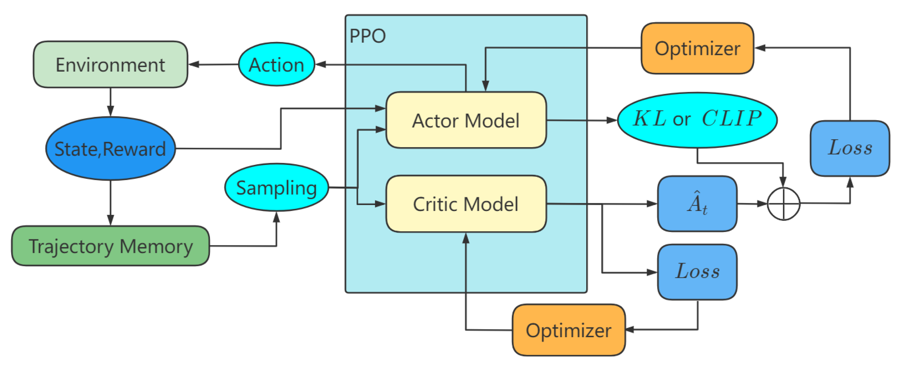
  • when using the dual Lagrangian method, a dynamically changing β value is used to constrain the update speed. The objective function is as follows:
    L K L ( θ ) = E ^ t [ π θ ( a t | s t ) π θ o l d ( a t | s t ) A ^ t β K L [ π θ o l d ( · | s t ) , π θ ( · | s t ) ] ]
    where π θ means the newest actor stochastic, π θ o l d means the newest strategy when taking samples, and A ^ t is the estimator of the advantage function of time t based on the current critic value function V φ k . During the training process, the value of β is changed depending on the expected value of the KL divergence. The formula is as follows:
    d = E ^ t [ K L [ π θ o l d ( · | s t ) , π θ ( · | s t ) ] ]
    Let d t a r g present the target value. If d is less than d t a r g / 1.5 , then β is reduced to a half. If d is greater than d t a r g × 1.5 , then β is doubled. Other conditions remain unchanged.
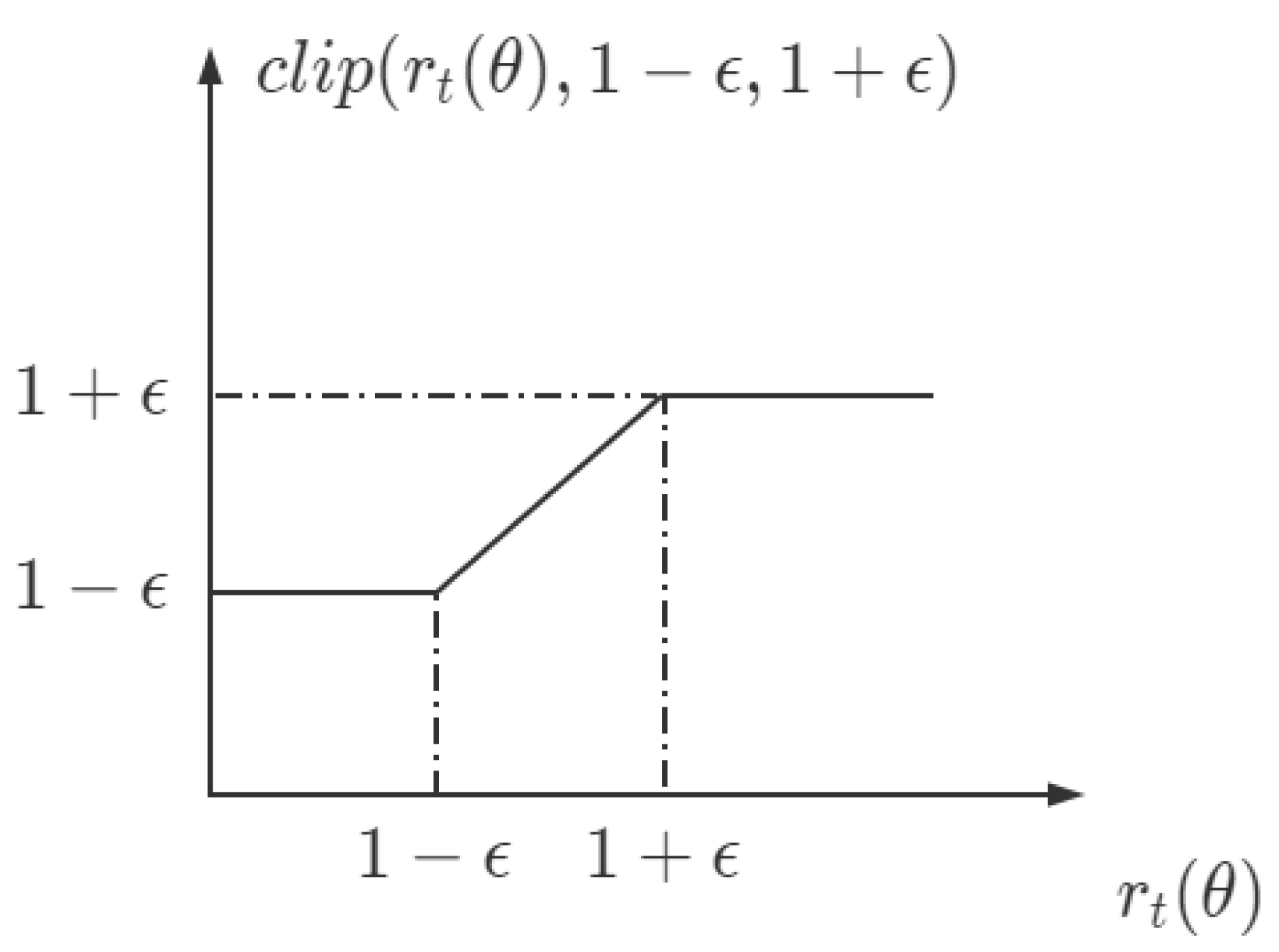
  • Use the clip function in Figure 3 to directly limit the difference between the output actions of the latest actor and the older actor. The probability ratio is as follows:
    r t ( θ ) = π θ ( a t | s t ) π θ o l d ( a t | s t )
    where θ denotes the current parameters of the actor neural network; θ old denotes the parameters at the time of sampling; and π θ ( a t | s t ) denotes the action probability of the actor output after inputting the observed states s t in which the parameters are. It is worth mentioning that due to the use of the LSTM neural network, the current actor output is influenced by the previously inputted observation states in the same input sequence, corresponding to the learning environment as the learning trajectory and feedback from all previous times during the complete learning process of a course. Therefore, the closer r t is to 1, the better. The reconstruction objective function is as follows:
    L C L I P ( θ ) = E ^ t [ m i n ( r t ( θ ) A ^ t , c l i p ( r t ( θ ) , 1 ϵ , 1 + ϵ ) A ^ t ) ]
    where ϵ is a custom constant, and the c l i p function limits the upper and lower bounds of the input.
Of the two methods, the training process is the same. Only some functions have changed. The training process is shown in Figure 4. The calculation method of the advantage value is the same. We previously mentioned that A ^ is obtained based on the value function. The value function is defined by the critic neural network. By putting the time t and state s t into the critic, we can obtain the value V ( s t ) at the current moment. The formula for calculating the advantage value is as follows:
A ^ t = ξ + ( γ λ ) ξ t + 1 + + + ( γ λ ) T t + 1 ξ T 1
where γ means the discount factor, T means the total of time, λ means the GAE parameter, and ξ is calculated by the following formula:
ξ = r t + γ V ( s t + 1 ) V ( s t )
where r t means the reward value given by the environment for the t-th action. v ( s t ) represents the evaluation value obtained when the input state is entered into the observed state s t similar to the actor, and the current output is influenced by the previous input.

3.6. Teaching Path Planning with DRL

In this section, we use DRL to deal with the teaching path planning problem.
First of all, based on the commonality between the student’s learning process and the student model, we define the entire class teaching process as a POMDP. We formulate this process through the four following points. Combined with the specific model, the parameters are defined as follows:
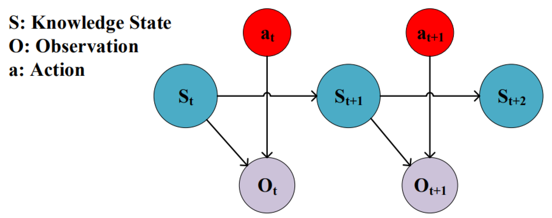
  • State Space: State Space S is all the possible states of all students in the class, that is, the possibilities for mastering a knowledge point. The difference is that for the EFC model, there are knowledge point difficulties, the times of learning, and the time after the last learning of each knowledge point. Contrary to the EFC model, the HLR model has no knowledge point difficulties and has a feature matrix. The feature matrix contains the times of the learned knowledge points, the times that knowledge points can be memorized, and the times that knowledge points cannot be recalled.
  • Observation Space: Because the teaching process is a POMDP, the real state cannot be obtained, and there is only one observation result, that is, the partial state. All possible states of this part constitute the Observation Space O, which is specifically all current real-time feedback, that is, whether the knowledge point is mastered. In actual teaching, real students obtain results by answering questions, etc. The model tests the samples through the following formula:
    O B e r n o u l l i ( S )
  • Action Space: The action space A is a collection of actions that can be acted upon, that is, knowledge points that teachers can choose to teach.
  • Transfer Function: The transfer function refers to the process of transforming state S t + 1 into state S t through action A. Specifically, after the teacher teaches, the class as whole changes state. In the EFC model, it changes the times of learning the knowledge point and the interval time between two times of learning. In the HLR model, it is similar to EFC, except that the feature matrix θ is additionally changed. The BKT model completes the state transition through Formula (9).
Both Long Short-Term Memory (LSTM) and Gate Recurrent Unit (GRU) are part of the most widespread recurrent neural networks today, and are both capable of learning long-distance dependencies. Through comparative experiments, the performance of the two is similar, but the LSTM training process is more stable in this environment. Therefore, as a continuous process, we use the PPO algorithm based on the LSTM neural network structure to solve the POMDP problem. Specifically, we use the ready-made implementation of the open source framework garage. We identify the two following points combining the above exact model and four constraints:
  • Reward Function: We define the player’s reward as the expected value of the test. The formula is as follows:
    g r a d e = i = 0 K P i
    In constraint 3, it can be seen that the overall reward is composed of three parts, as shown in the following formula:
    R e w a r d = a 0 R p + a 1 R e + a 2 R a
    R p = m i n ( m · p , n u m ( p a s s ) )
    R p = m i n ( m · e , n u m ( e x c e l l e n t ) )
    R a = i = 0 m g r a d e i / m
    where R p represents the pass rate reward, R e represents the excellent rate reward, R a represents the average score reward, n u m ( p a s s ) represents the number of students who passed the test, and n u m ( e x c e l l e n t ) represents the number of students with excellent test scores. We consider the logarithmic reward, for which the formula is as follows:
    R e w a r d = l o g ( a 0 R p + a 1 R e + a 2 R a )
  • Discount factor: The discount factor determines whether to pay more attention to current returns or long-term returns. In the teaching process, we usually pay more attention to the teaching income at any time, so a large discount factor is better.
The observation space, the sequence of knowledge points learned, and the current time together constitute the input of the LSTM. The output is the next knowledge point to be learned. The procedure of the PPO algorithm is shown in Algorithm 1:
Algorithm 1 PPO-Clip
1:
Initial policy parameters θ 0 and value function parameters φ 0
2:
for k = 1 to N do
3:
    for  i = 1 to M do
4:
        Run policy π k = π ( θ k ) in environment for T time steps
5:
        Compute advantage estimates A ^ i based on the current value function V φ k
6:
    end for
7:
    Collect set of trajectories D k = τ i
8:
    Update the policy by maximizing the objective:
θ k + 1 = a r g m a x θ 1 | D k | T τ D k t = 0 T m i n ( π θ ( a t | s t ) π θ k ( a t | s t ) A π θ k ( S t , a t ) , g ( ϵ , A π θ k ( S t , a t ) ) )
    via stochastic gradient ascent with Adam
9:
    Fit value function by regression on mean-squared error:
φ k + 1 = a r g m i n φ 1 | D k | T τ D k t = 0 T ( V φ ( s t ) R ^ t ) 2
    via stochastic gradient ascent with Adam
10:
end for
  • First, we initialize various parameters and then train through K iterations. In a training iteration, collecting samples is the primary activity, which uses an actor neural network to generate a strategy to capture a period of an environmental change trajectory. In our algorithm, the actor neural network used to generate the strategy and the critic neural network used to calculate the value are both LSTM. The input of the actor is the sequence of the observation space of the whole class, the knowledge points of the previous teaching, and the time interval from the previous teaching. The output is the currently selected teaching knowledge point sequence. After receiving the knowledge that it is about to be taught, the environment model returns the teaching observation and reward. At the time of sample collection, the specific data of the sample are the current observation, the knowledge point for teaching, the observation after teaching, and the reward obtained.
  • According to the collected data, the advantage value is calculated through a critic neural network. The input of the critic is the same as the actor, and the output value is used to calculate the advantage. Then, we train the actor neural network based on Line 8.
  • Then we use Line 9 to train the critic neural network.
  • Looping the above steps k times is a complete training process.
It is worth mentioning that we used the same random projection method as in [20] to reduce the input dimension so that a larger number of knowledge points can be processed.

4. Experiments

In this section, we introduced the experimental design in detail and analyzed the experimental results to verify the effectiveness of the method proposed in this article through various comparisons.

4.1. Experimental Setup

We introduced three models in the teaching path planning to simulate students’ experiential learning and DRL. We set up four strategies for comparison:
  • Random method: Random method is completely random when selecting a recommended knowledge point, and is the most common.
  • Linear method: Linear method seeks to evenly allocate time to each knowledge point and then teach in the order of knowledge points. This is the most widespread method in traditional classrooms.
  • Cyclic method: Cyclic method means that after learning all the knowledge points one by one, if there is still time, re-learn the first knowledge point and repeat.
  • Threshold method: The threshold method is a cheating method. It directly reads the explicit content of the student model and selects the knowledge point with the lowest average mastery.
We set the number of students to 20, knowledge points to 25, class times to 80, and 5 time units between each class. The results of the experiment are reflected by the number of qualified students in the class, the number of outstanding students in the class, and the average mastery of knowledge points. When a student’s average mastery of all knowledge points exceeds 0.6, we think that they can pass, and when it exceeds 0.8, we think that they are excellent. The parameter { a 0 , a 1 , a 2 } in the Formula (22) and (26) are set to { 5 , 3 , 1 } .
To have a reasonable class score distribution, for the EFC model, we set the level distribution of class students as l e v e l N ( 4 , 2 ) with an upper limit of 1 , and the learning difficulty of the knowledge points corresponding to each student is θ N ( l e v e l , 2 ) with an upper limit of 0. We used Formulas (22) and (26) as the reward functions for training, and the results are shown in Table 1. When we canceled the knowledge point association, since there is no restriction on the association between knowledge points, we set the level distribution of class students as l e v e l N ( 2.6 , 2 ) . The experimental results are shown in Table 2.
For the HLR model, we set the level distribution of class students as l e v e l N ( 0.7 , 3 ) with a lower limit of 0, and the memory strength parameter corresponding to each student is θ = ( 1 , 1 , 0 , θ 0 N ( l e v e l , 2 ) ) . Furthermore, Formulas (22) and (26) were used as the reward functions for training, and the results are shown in Table 3. When we canceled the knowledge point association, the experimental results are shown in Table 4.
For the BKT model, we set the level distribution of class learning as l e v e l N ( 0.5 , 1 ) , and the learning difficulty of the knowledge points corresponding to each student is l N ( l e v e l , 1 ) with an upper limit of 0.7 and a lower limit of 0.2 . We use the same method in experiments, and the results are presented in Table 5. When we canceled the knowledge point association, since the BKT model has no forgetting mechanism, we set class times to 40. The experimental results are shown in Table 6.
We set the batch size to 4000, the hidden layer size to 32, the discount rate to 0.99, the GAE parameter to 0.95, and the step size to 0.001.
Finally, we verified the effect of multi-target settings. We numbered the three sub-rewards of Formula (22) in order, as shown in Table 7 and then recombined them into the rewards given to training by the DRL environment. The results are shown in Table 8.

4.2. Results

Table 1, Table 2, Table 3, Table 4, Table 5 and Table 6 show the experimental results of the three models. The experimental results are divided into two parts, with Formulas (22) and (26) as the objective function, respectively. The results of each part consist of the following parts:
  • The average value of the average mastery of knowledge points of each student in the class;
  • The number of students whose average mastery of knowledge points exceeds 0.6;
  • The number of students whose average mastery of knowledge points exceeds 0.8;
  • The standard deviation of the average mastery of knowledge points in the class.
For the EFC model, it can be observed in Table 1 that the DRL method is significantly better than the random and linear methods. DRL is similar to cyclic and threshold methods. When Formula (26) is used as the objective function, DRL has a better effect. At the same time, the standard deviation of DRL-based students’ performance is the smallest in all cases. Table 2 shows the results after disassociating the knowledge points. The general situation is the same as in Table 1. The DRL method also performs better when Formula (22) is used as the objective function.
The effect of the HLR model implemented in Table 3 differs from that of the EFC model. The effect of the linear method was improved. DRL achieved the best results in terms of average grade, pass rate, excellent rate, and standard deviation. When we cancelled the knowledge point association, the result shown in Table 4 was obtained. The effect of linear teaching was greatly improved. The DRL method was second only to the linear method.
Table 5 shows that the DRL method is superior to other methods in all aspects of the BKT model. When we canceled the knowledge point association, it can be observed in Table 6 that the DRL method did not differ greatly from the other methods. This is because the BKT model does not consider the forgetting strategy, so four methods can obtain a good result.
After experimenting with a random combination of multiple targets, the result in Table 7 shows that adding each sub-reward to the reward of Formula (22) will improve the effect of DRL, which proves that the reward function we proposed is both reasonable and effective. Through the above experiments, it can be seen that each of the four comparison strategy methods have advantages and disadvantages. In contrast, DRL achieves good results in all cases. In some of the experiments, DRL did not obtain the best teaching results but obtained higher rewards due to the algorithm setting a larger discount factor to quickly improve the performance in the early stage to improve the overall rewards. The effectiveness of DRL does not depend on a specific context, which proves the efficiency and generality of the method. Furthermore, a multi-part randomized combination experiment verified that each part of the reward function setting was beneficial. Thus, DRL, as the group teaching recommendation algorithm used in the system, can meet the system design requirements for this recommendation function.

4.3. Discussion

Through the above experiments, it can be seen that the four comparison methods have their own advantages and disadvantages. In contrast, DRL can achieve good results in any situation. The effect of DRL does not depend on a specific environment, which proves the efficiency and versatility of the method. At the same time, the random combination experiment of multiple parts verifies that each part of the reward function setting is beneficial. In addition, due to the high discount factor we set, DRL will achieve a better result at the fastest speed and slow down the speed of improvement in the later stage.

5. Cloud Computing Assisted

Various teaching aids are necessary to facilitate teaching interactions and the better utilization of the built student models during or after the classroom. Their integration of advanced technologies in the fields of mobile computing, pervasive computing, communication technologies, augmented reality, sensors, artificial intelligence, and data mining provides a wide range of classroom interactions based on these technologies. Considering that there are more functions in the system and machine learning algorithms, it is difficult for the single-server architecture to load the system operation pressure, so the system adopts a distributed architecture. The system is divided into different microservices according to the functional modules, and multiple microservices can run on different servers and call each other through pre-designed interfaces to complete the teaching assistants work together. The server side of the system adopts the development method of front and back-end separation: the back-end part adopts the distributed architecture based on the SpringCloud framework, and the development language is JAVA; the front-end part is developed based on the Vue framework; the client side is based on Android platform, and the development language is JAVA, and the database uses Mysql; the server side is deployed on a Linux server.

6. Conclusions

In this article, we studied how to arrange the teaching path of teachers within a limited time course, considering the different situations of different students and the interrelationship between knowledge points. Most of the current related work focuses on students’ learning path planning. We are the first to study teacher-oriented teaching planning based on the entire teaching semester and the entire class. Our research goal is to make the entire class benefit from this course as much as possible, which is embodied in the passing rate, excellence rate, and the average score of the class for the exam. For this problem, we proposed the use of DRL to generate strategies through neural networks. We utilized a variety of student models to conduct simulation experiments and achieved excellent experimental results. This proves that this method can be applied to various environments and is widely operative.
In this article, the first limitation is that there are no experiments based on real students. Real-life tests will bring some new problems, such as how to better obtain feedback from students without affecting students’ learning, how to confirm the accuracy of students’ feedback, and how to eliminate errors. At the same time, our experiments were built on the assumptions in Section 3.1, which only consider the perfect condition that all learning details are captured by the system. In real-life tests, the teacher and students may have many problems with Blended Learning that leave some learning details unobserved by the system. Thus, real-life tests and related optimization based on partially observed facts will be our next research agenda.

Author Contributions

Conceptualization, N.L. and L.Z.; Data curation, T.Y. and X.Y.; Formal analysis, T.Y. and X.Y.; Funding acquisition, L.Z.; Investigation, T.Y. and X.Y.; Methodology, T.Y. and X.Y.; Project administration, N.L. and L.Z.; Resources, N.L. and L.Z.; Software, T.Y. and X.Y.; Supervision, T.Y. and X.Y.; Validation, T.Y. and X.Y.; Visualization, T.Y. and X.Y.; Writing—original draft, T.Y.; Writing—review and edition, N.L. and L.Z. All authors have read and agreed to the published version of the manuscript.

Funding

This work was supported by the National Natural Science Foundation of China under Grant 61572113 and Grant 61877009.

Institutional Review Board Statement

This study was conducted according to the guidelines of the Declaration of Helsinki and approved by the Institutional Review Board of University of Electronic Science and Technology of China.

Informed Consent Statement

Informed consent was obtained from all individual participants included in the study.

Data Availability Statement

Not applicable.

Acknowledgments

The authors would like to thank Kedi Chen for valuable and constructive suggestions and discussions.

Conflicts of Interest

The funder had no role in the study design, data collection, data analysis, data interpretation, or writing of the report.

Abbreviations

The following abbreviations are used in this manuscript:
IOTInternet of Things
DRLDeep Reinforcement Learning
DDPGDeep Deterministic Policy Gradient
AALAmbient-assisted living
BSBase station

References

  1. Stowell, J.R. Use of clickers vs. mobile devices for classroom polling. Comput. Educ. 2015, 82, 329–334. [Google Scholar] [CrossRef]
  2. Ceven McNally, J. Learning from one’s own teaching: New science teachers analyzing their practice through classroom observation cycles. J. Res. Sci. Teach. 2016, 53, 473–501. [Google Scholar] [CrossRef]
  3. Shou, Z.; Lu, X.; Wu, Z.; Yuan, H.; Zhang, H.; Lai, J. On learning path planning algorithm based on collaborative analysis of learning behavior. IEEE Access 2020, 8, 119863–119879. [Google Scholar] [CrossRef]
  4. Xie, H.; Zou, D.; Wang, F.L.; Wong, T.L.; Rao, Y.; Wang, S.H. Discover learning path for group users: A profile-based approach. Neurocomputing 2017, 254, 59–70. [Google Scholar] [CrossRef]
  5. Ebbinghaus, H. Memory: A contribution to experimental psychology. Ann. Neurosci. 2013, 20, 155. [Google Scholar] [CrossRef]
  6. Settles, B.; Meeder, B. A trainable spaced repetition model for language learning. In Proceedings of the 54th Annual Meeting of the Association for Computational Linguistics (Volume 1: Long Papers), Berlin, Germany, 7–12 August 2016; pp. 1848–1858. [Google Scholar]
  7. Zaidi, A.; Caines, A.; Moore, R.; Buttery, P.; Rice, A. Adaptive forgetting curves for spaced repetition language learning. In Proceedings of the International Conference on Artificial Intelligence in Education, Ifrane, Morocco, 6–10 July 2020; pp. 358–363. [Google Scholar]
  8. Corbett, A.T.; Anderson, J.R. Knowledge tracing: Modeling the acquisition of procedural knowledge. User Model. User-Adapt. Interact. 1994, 4, 253–278. [Google Scholar] [CrossRef]
  9. Van De Sande, B. Properties of the Bayesian Knowledge Tracing Model. J. Educ. Data Min. 2013, 5, 1–10. [Google Scholar]
  10. Piech, C.; Spencer, J.; Huang, J.; Ganguli, S.; Sahami, M.; Guibas, L.; Sohl-Dickstein, J. Deep knowledge tracing. arXiv 2015, arXiv:1506.05908. [Google Scholar]
  11. Ding, X.; Larson, E.C. Incorporating uncertainties in student response modeling by loss function regularization. Neurocomputing 2020, 409, 74–82. [Google Scholar] [CrossRef]
  12. Lu, X.; Zhu, Y.; Xu, Y.; Yu, J. Learning from multiple dynamic graphs of student and course interactions for student grade predictions. Neurocomputing 2021, 431, 23–33. [Google Scholar] [CrossRef]
  13. Rafferty, A.N.; Brunskill, E.; Griffiths, T.L.; Shafto, P. Faster teaching via pomdp planning. Cogn. Sci. 2016, 40, 1290–1332. [Google Scholar] [CrossRef]
  14. Elshani, L.; Nuçi, K.P. Constructing a personalized learning path using genetic algorithms approach. arXiv 2021, arXiv:2104.11276. [Google Scholar]
  15. Niknam, M.; Thulasiraman, P. LPR: A bio-inspired intelligent learning path recommendation system based on meaningful learning theory. Educ. Inf. Technol. 2020, 25, 3797–3819. [Google Scholar] [CrossRef]
  16. Reddy, S.; Labutov, I.; Banerjee, S.; Joachims, T. Unbounded human learning: Optimal scheduling for spaced repetition. In Proceedings of the 22nd ACM SIGKDD International Conference on Knowledge Discovery and Data Mining, San Francisco, CA, USA, 13–17 August 2016; pp. 1815–1824. [Google Scholar]
  17. Hoi, S.C.; Sahoo, D.; Lu, J.; Zhao, P. Online learning: A comprehensive survey. arXiv 2018, arXiv:1802.02871. [Google Scholar] [CrossRef]
  18. Wang, S.; Xu, Y.; Li, Q.; Chen, Y. Learning Path Planning Algorithm Based on Learner Behavior Analysis. In Proceedings of the 2021 4th International Conference on Big Data and Education, London, UK, 3–5 February 2021; pp. 26–33. [Google Scholar]
  19. Shi, D.; Wang, T.; Xing, H.; Xu, H. A learning path recommendation model based on a multidimensional knowledge graph framework for e-learning. Knowl.-Based Syst. 2020, 195, 105618. [Google Scholar] [CrossRef]
  20. Reddy, S.; Levine, S.; Dragan, A. Accelerating human learning with deep reinforcement learning. In Proceedings of the NIPS’17 Workshop: Teaching Machines, Robots, and Humans, Long Beach, CA, USA, 9 December 2017; pp. 5–9. [Google Scholar]
  21. Sinha, S. Using Deep Reinforcement Learning for Personalizing Review Sessions on e-Learning Platforms with Spaced Repetition. 2019. Available online: https://www.semanticscholar.org/paper/Using-deep-reinforcement-learning-for-personalizing-Sinha/3f73a776916f491f18a24576ac352c63bd533040 (accessed on 2 August 2022).
  22. Ghiani, G.; Manni, E.; Romano, A. Training offer selection and course timetabling for remedial education. Comput. Ind. Eng. 2017, 111, 282–288. [Google Scholar] [CrossRef]
  23. Muhammad, I.; Azhar, I.M.; Muhammad, A.; Arshad, I.M. SIM-Cumulus: An Academic Cloud for the Provisioning of Network-Simulation-as-a-Service (NSaaS). IEEE Access 2018, 6, 27313–27323. [Google Scholar]
  24. Ibrahim, M.; Nabi, S.; Baz, A.; Naveed, N.; Alhakami, H. Toward a Task and Resource Aware Task Scheduling in Cloud Computing: An Experimental Comparative Evaluation. Int. J. Netw. Distrib. Comput. 2020, 8, 131–138. [Google Scholar] [CrossRef]
  25. Wang, Z.; Wan, Y.; Liang, H. The Impact of Cloud Computing-Based Big Data Platform on IE Education. Wirel. Commun. Mob. Comput. 2022, 2022, 1–13. [Google Scholar] [CrossRef]
  26. Tai, B.; Li, X.; Yang, L.; Miao, Y.; Lin, W.; Yan, C. Cloud Computing-aided Multi-type Data Fusion with Correlation for Education. Wirel. Netw. 2022, 1–12. [Google Scholar] [CrossRef]
  27. Zhao, J. Construction of College Chinese Mobile Learning Environment Based on Intelligent Reinforcement Learning Technology in Wireless Network Environment. Wirel. Commun. Mob. Comput. 2022, 2022, 5164430. [Google Scholar] [CrossRef]
  28. Siemens, G.; Gašević, D.; Dawson, S. Preparing for the Digital University: A Review of the History and Current State of Distance, Blended, and Online Learning; Athabasca University Press: Athabasca, AB, Canada, 2015. [Google Scholar]
  29. Nikou, S.A.; Economides, A.A. Mobile-based assessment: Investigating the factors that influence behavioral intention to use. Comput. Educ. 2017, 109, 56–73. [Google Scholar] [CrossRef]
  30. Anshari, M.; Almunawar, M.N.; Shahrill, M.; Wicaksono, D.K.; Huda, M. Smartphones usage in the classrooms: Learning aid or interference? Educ. Inf. Technol. 2017, 22, 3063–3079. [Google Scholar] [CrossRef]
  31. Han, J.H.; Finkelstein, A. Understanding the effects of professors’ pedagogical development with Clicker Assessment and Feedback technologies and the impact on students’ engagement and learning in higher education. Comput. Educ. 2013, 65, 64–76. [Google Scholar] [CrossRef]
  32. Kim, I.; Kim, R.; Kim, H.; Kim, D.; Han, K.; Lee, P.H.; Mark, G.; Lee, U. Understanding smartphone usage in college classrooms: A long-term measurement study. Comput. Educ. 2019, 141, 103611. [Google Scholar] [CrossRef]
  33. Sung, Y.T.; Chang, K.E.; Liu, T.C. The effects of integrating mobile devices with teaching and learning on students’ learning performance: A meta-analysis and research synthesis. Comput. Educ. 2016, 94, 252–275. [Google Scholar] [CrossRef]
  34. Burden, K.; Kearney, M.; Schuck, S.; Hall, T. Investigating the use of innovative mobile pedagogies for school-aged students: A systematic literature review. Comput. Educ. 2019, 138, 83–100. [Google Scholar] [CrossRef]
  35. Chung, C.J.; Hwang, G.J.; Lai, C.L. A review of experimental mobile learning research in 2010–2016 based on the activity theory framework. Comput. Educ. 2019, 129, 1–13. [Google Scholar] [CrossRef]
  36. Schulman, J.; Wolski, F.; Dhariwal, P.; Radford, A.; Klimov, O. Proximal policy optimization algorithms. arXiv 2017, arXiv:1707.06347. [Google Scholar]
  37. Xie, T.; Cheng, X.; Wang, X.; Liu, M.; Deng, J.; Zhou, T.; Liu, M. Cut-Thumbnail: A Novel Data Augmentation for Convolutional Neural Network. In Proceedings of the 29th ACM International Conference on Multimedia, Virtual Event, 20–24 October 2021; pp. 1627–1635. [Google Scholar]
Figure 1. Partially observable Markov decision process [8].
Applsci 12 09376 g001
Figure 2. (I) The teacher teaches a knowledge point; (II) The students study it with the changes in their student states; (III) The results of in-class and off-class tests for students are observed. During the continuous teaching process, a knowledge point chain, a student state chain, and a student test result chain are formed.
Applsci 12 09376 g002
Figure 3. Clip function.
Applsci 12 09376 g003
Figure 4. PPO: (I) Sampling by actor; (II) the collected data are sampled again and passed to the actor and critic; and (III) updating through the two different loss functions.
Applsci 12 09376 g004
Table 1. The results of EFC that consider the knowledge points association.
MethodAveragePassExcellentSDAverage (log)Pass (log)Excellent (log)SD (log)
Random0.319300.2220.353510.255
Linear0.229200.2130.308310.265
Cyclic0.443630.2550.522830.276
Threshold0.428630.2580.489730.289
DRL0.438630.2470.500930.241
Table 2. The results of EFC that do not consider the knowledge point association.
MethodAveragePassExcellentSDAverage (log)Pass (log)Excellent (log)SD (log)
Random0.462520.2010.366320.208
Linear0.413420.2050.309310.218
Cyclic0.557830.2120.451420.220
Threshold0.556730.2130.451420.224
DRL0.485820.2040.396520.225
Table 3. The results of HLR that consider the knowledge point association.
MethodAveragePassExcellentSDAverage (log)Pass (log)Excellent (log)SD (log)
Random0.271410.2520.209100.173
Linear0.412540.3000.377520.284
Cyclic0.422540.2880.373530.269
Threshold0.347430.2990.312510.280
DRL0.503740.2370.564640.285
Table 4. The results of HLR that do not consider the knowledge point association.
MethodAveragePassExcellentSDAverage (log)Pass (log)Excellent (log)SD (log)
Random0.525640.2070.490610.170
Linear0.6801250.1730.645860.169
Cyclic0.586840.2230.514650.239
Threshold0.582840.2330.514650.236
DRL0.6251240.2120.540850.227
Table 5. The results of BKT that consider the knowledge point association.
MethodAveragePassExcellentSDAverage (log)Pass (log)Excellent (log)SD (log)
Random0.470300.1110.461400.119
Linear0.6301040.1470.536800.151
Cyclic0.620940.1440.560820.156
Threshold0.599820.1440.595820.157
DRL0.6431240.1500.5921030.152
Table 6. The results of BKT that do not consider the knowledge point association.
MethodAveragePassExcellentSDAverage (log)Pass (log)Excellent (log)SD (log)
Random0.553700.0960.528600.110
Linear0.6241230.1200.575710.121
Cyclic0.6331330.1230.580810.126
Threshold0.6331330.1240.583810.127
DRL0.6331230.1230.581810.126
Table 7. Component definition.
Num123
Name R p R e R a
Table 8. Component comparison experiment.
MethodAveragePassExcellent
120.40553
130.40660
230.42962
DRL(123)0.43763
Publisher’s Note: MDPI stays neutral with regard to jurisdictional claims in published maps and institutional affiliations.

