DRUNet: A Method for Infrared Point Target Detection

Abstract

Deep learning is widely used in vision tasks, but feature extraction of IR small targets is difficult due to the inconspicuous contours and lack of color information. This paper proposes a new convolutional neural network–based (CNN-based) method for IR small target detection called DRUNet. The algorithm is divided into two parts: the feature extraction network and the prediction head. For the small IR targets, which are difficult to accurately label, Gaussian soft labels are added to supervise the training process and make the network converge faster. We use a simplified object keypoint similarity to evaluate the network accuracy by the ratio of the distance to the radius of the inner tangent circle of the target box and a fair method for evaluating the model inference speed after GPU preheating. The experimental results show that our proposed algorithm performs better when compared with commonly used algorithms in the field of small target detection. The model size is 10.5 M, and the test speed reaches 133 FPS under the RTX3090 experimental platform.

1. Introduction

Infrared detection technology has the characteristics of noncontact and passive detection. Compared with visible image detection, infrared detection technology is less affected by light conditions. Infrared detection technology has the advantages of strong survivability and good portability and can achieve the detection of radar blind areas [1]. Infrared detection and tracking of small targets are widely used in military and maritime fields, such as early warning systems and precision guidance [2]. In recent years, with the development of infrared imaging devices and the popularity of Internet of Things technology, more and more applications have emerged, such as video surveillance, robotic visual navigation, and medical diagnosis [3]. The task of target detection is to be able to identify the category of the target and the location of the target in the given picture or video, which is the basis for tasks such as target tracking. Therefore, research of detection and tracking of infrared small targets has attracted the attention of many scholars. Infrared small targets are characterized by smallness and dimness. Small means that the ratio of pixels occupied by the target to the pixels of the picture is low, and according to the definition of the International Society of Photo-Optical Instrumentation Engineers (SPIE) [4], any target whose size is less than 0.12% of the entire imaging area can be called a small target (i.e., when the image size is 256 × 256, the small targets should have no more than 81 pixels, and their target size should be within 9 × 9). Dimness refers to the intensity of the target in the infrared wavelengths, specifically reflected in the captured infrared image, and refers to the gray value of the target, which, after imaging the target, may not be the brightest area of the image.

To solve the problem of small target detection, scholars have proposed many methods. These methods can generally be divided into two categories: single-frame detection and multiframe detection. Both types of algorithms have their advantages and disadvantages [5]. Single-frame detection algorithms generally have higher miss and false detection rates than multiframe detection algorithms. Multiframe detection algorithms are usually more time-consuming than single-frame detection algorithms, and multiframe detection algorithms generally assume a static background, which makes multiframe detection algorithms unsuitable for many moving camera applications [6].

Single-frame detection methods can be further divided into traditional methods and convolutional neural network–based (CNN-based) detection methods [7]. Traditional single-frame-based image detection algorithms are broadly classified into three types of algorithms based on filtering [8,9,10,11], local contrast [12,13,14], and nonlocal self-similarity [15], based on the a priori characteristics of their models. These methods are usually more susceptible to clutter and noise in the background, have insufficient discrimination of scene changes, and are hyperparametrically sensitive, which affects the robustness of detection. Another method is the CNN-based approach; it holds an advantage in the small target detection capability and segmentation integrity.

Based on this, we propose a CNN-based infrared small target detection algorithm, which treats small targets as a key point detection task. Experimental validation and performance evaluation were conducted, and the experimental results showed that the algorithm has good performance.

The contributions of this paper are as follows:

• An effective CNN-based infrared small target detection algorithm is proposed, containing a feature extraction module and a prediction head module, where the feature extraction part can be used for other infrared small target vision tasks.
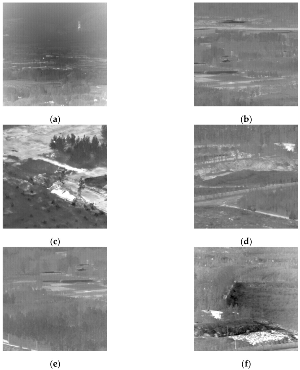
• For the problem of a sparse infrared small target dataset, the publicly available infrared small target dataset is expanded by selecting images with large target variations from the infrared tracking dataset using the frame extraction method.
• An evaluation method for keypoint detection and a fair method to measure the inference speed of the network are proposed.

2. Related Work

2.1. Infrared Single-Frame Small Target Detection by CNN-Based Method

Zhao et al. [16] proposed IR small target detection with a generative adversarial network (IRSTD-GAN) in 2021, using a generative adversarial network, where the generator outputs the grayscale prediction of the target and trains the discriminator for indirect supervision while directly supervising it. Dai et al. [17] proposed the asymmetric contextual modulation (ACM) algorithm, which contrasts the fusion between deep and low-level features and proposes an asymmetric contextual modulation module. The high semantic features use the channel attention feature weight distribution for the low-level features, and the low-level features use the pointwise convolution spatial attention to distribute the feature weights for the high semantic features. Attentional local contrast (AlcNet) was proposed in the paper [18] to address the problem of intrinsic features in a purely data-driven approach, using a model-driven combined with a data-driven approach, inputting the multilevel feature map of the network into a nonparametric nonlinear local contrast model and then performing fusion regression, and performing enhancement or suppression operations on different regions of the feature map based on small target characteristics. The author also discloses the single-frame small infrared target (SIRST) dataset used, which is also used in our training and experiments. Li et al. [19] proposed dense nested attention network for IR small target detection (DNAnet). They designed a densely nested interaction module (DNIM) to implement progressive interactions between high-level and low-level features. Using repetitive interactions in DNIM, deep IR small targets can be maintained. Based on DNIM, a cascaded channel and spatial attention module (CSAM) is further proposed to adaptively enhance multilevel features, which can integrate and fully utilize the contextual information of small targets by iterative fusion and enhancement. Zuo et al. [20] designed the attention fusion feature pyramid network (AFFPN) specifically for small infrared target detection. It consists of feature extraction and feature fusion modules. In the feature extraction stage, the global contextual prior information of small targets is first considered in the deep layer of the network using the atrous spatial pyramid pooling module. Subsequently, the spatial location and semantic information features of small infrared targets in the shallow and deep layers are adaptively enhanced by the designed attention fusion module to improve the feature representation capability of the network for targets. Finally, high-performance detection is achieved through the multilayer feature fusion mechanism.

Although the performance of the CNN-based method has improved in recent years, the problem of small target loss remains. The complexity of some models is relatively high, and there is still space for optimization in terms of detection rate and detection efficiency [21].

2.2. Object Detection by Keypoint Estimation

To detect small IR targets, the prediction head uses a keypoint detection mechanism. There are two main ideas for the anchor-free model based on keypoints: one is grouping keypoints at a specific location, and the other is combining the central keypoints for regression prediction. The anchor-free model based on keypoint grouping detects specific keypoints from the feature map and generates high-quality detection frames based on matching keypoints, reducing the problems of feature mismatch and computational redundancy of predefined anchor frames. Such models include CornerNet [22] based on corner points and its optimized version CornerNet-Lite [23], ExtremeNet [24] based on extreme points, and so on. The anchor-free model that combines the central keypoints outputs the probability of it being the target centroid, the regression target scale, and the offset at each position of the feature map for the prediction of the edges. CenterNet [25] and series work are two examples of such models. To solve the problem of CornerNet, ExtremeNet relies on the postprocessing step of grouping keypoints, which reduces the detection speed. CenterNet provides a more concise idea of extracting the centroids of each target without grouping multiple keypoints. Similar to the anchor-based algorithm, CenterNet analogizes the centroid to a single anchor of an unknown shape. Because this anchor is only position related, there is no overlapping of anchors and no need to set artificial thresholds to distinguish between foreground and background. In terms of the design of the detection process, CenterNet does not postprocess the grouping of keypoints, thus greatly reducing the number of network parameters and computational effort.

3. Proposed Network

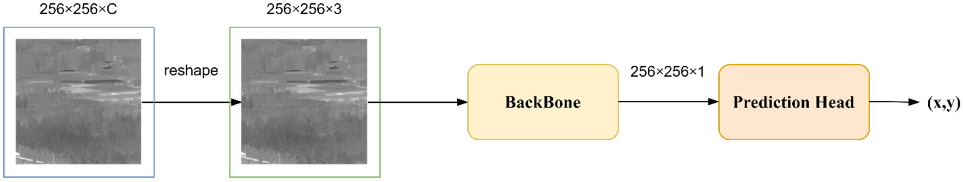
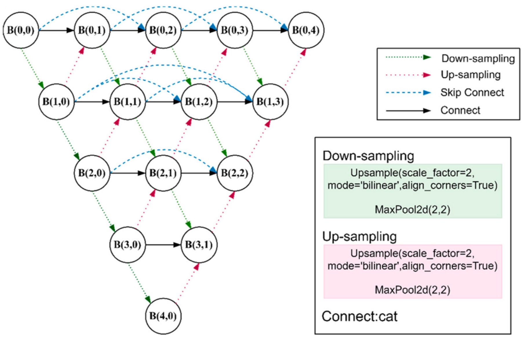
3.1. Network Architecture

CNN-based methods for detecting small infrared targets face two main challenges.

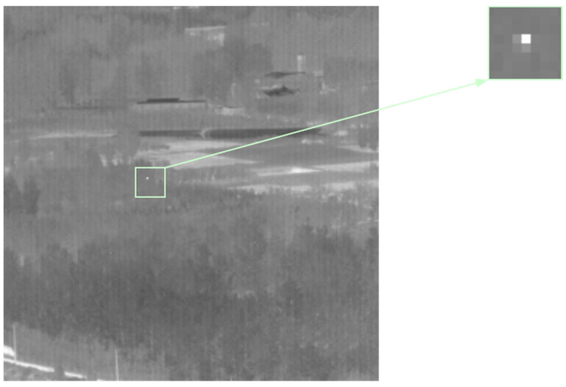
• Unlike visible images, infrared images lack information, such as color, texture, and contours, especially in deep networks, where small targets are easily overwhelmed by complex environments or confused with pixel-level impulse noise.
• Resolution and semantics conflict. A complex low SNR ratio background often obscures small infrared targets. Deep networks learn more semantic representations by gradually shrinking feature sizes, which is inherently counterintuitive because they are learning more semantic representations by gradually decaying the feature size. To detect these small targets with a low false alarm rate, the network must have a high-level semantic understanding of the whole IR image.

In this paper, the network design is considered from three aspects for the detection task of small infrared targets.

• Down-sampling scheme: Many studies emphasize that the acceptance domain of predictors should match the target scale range when designing CNNs. If the down-sampling scheme is not recustomized, it is difficult to retain the features of small IR targets as the network goes deeper [26]. Therefore, our proposed method maintains an up-sampling rate of 2 and a down-sampling rate of 0.5 when performing feature extraction.
• Suitable image attention enhancement module: Since ordinary visible image targets are relatively large and the pixels occupied by the targets are more widely distributed in the graph, the existing attention modules tend to aggregate global or long-term contexts. However, infrared small targets occupy fewer pixels, so it is necessary to choose the appropriate module when using attention modules; otherwise, it is impossible to optimize the network performance while increasing the model complexity.
• Feature fusion methods: Feature fusion is mostly studied in a one-way, top–down manner to fuse cross-layer features and to select appropriate low-level features based on high-level semantics. However, only using top-down modulation may not work because small targets may already be overwhelmed by the background.

Based on the above three points, we propose an effective IR small target detection algorithm called DRUNet (Dense-Rest-UNet) network. Figure 1 shows the overall structure of the algorithm proposed in this paper; it can be divided into two parts: the feature extraction network and the prediction head. The feature extraction network structure is similar to the dense nested network structure of UNet++ [27], but unlike UNet++, we propose an attention enhancement module based on the residual structure called ECA-Rest Block, which becomes the base block of the dense nested network. We design the prediction head to predict the feature map obtained from the feature extraction network and generate a heatmap to predict the coordinates of the target location. The next part of this section will explain each part of the algorithm in detail.

3.2. ECA-Rest Block

The feature extraction network proposed in this paper uses a skip connect between each node of the densely nested network structure in addition to the intranode skip connect, which is a residual structure. The residual structure has two obvious features: One is forward propagation enables the low-level features to be reused, preserving more low-level features for better feature extraction of small targets. Another is backward propagation, where the gradient of the deeper layer can be directly passed back to the shallow layer, preventing the problem of network degradation and difficulty in training as the network deepens. In addition, to better enhance the target information, we add an image attention enhancement module with a simple and effective structure. We also use the normalization layer to solve the problem of the possible gradient explosion and gradient disappearance problems.

Efficient channel attention (ECA) is an efficient channel attention module proposed by Wang et al. for image attention enhancement, which involves only a small number of parameters while having obvious performance gains. Appropriate cross-channel interactions can significantly reduce model complexity while maintaining performance [28]. The specific operation of the ECA module is as follows: After global average pooling, the information interaction between channels is completed through one-dimensional convolution (1D-Conv). The size of the convolution kernel of the 1D-Conv is adapted by Equation (2) so that layers with a larger number of channels can perform more cross-channel interactions. In the feature extraction network, the number of channels is usually a power of 2, so there is a mapping Equation (1) between the convolution kernel size K and the number of channels C, where $\gamma$ and b are constants:

$$C=\mathsf{\Phi }\left(k\right)=2^{\left(\gamma \times k-b\right)},$$

(1)

The formula for calculating the size of the adaptive convolution kernel is:

$$k=\mathsf{\Psi }\left(C\right)={\left|\frac{{\log }_2\left(C\right)}{\gamma }+\frac{b}{\gamma }\right|}_{odd},$$

(2)

${\left|t\right|}_{odd}$ represents the nearest odd number for t. $\gamma$ is set to 2, and b is set to 1, which is the original setting of the ECA module.

The ECA schematic is shown in Figure 2.

The structure of the ECA-Rest Block is shown in Figure 3, and Input is the output from other nodes after concatenation in dimension 1. For example, assuming that the nodes on the same level in the feature extraction network are nodes on the same level, the feature maps of the three ways of the L(0, 2) input come from the feature maps of L(0, 0) and L(0, 1) on the same level and L(1, 0) on a different level after up-sampling, and the size of the feature maps on the same level is (batch size, 16, 256, 256), and the size of the L(1, 0) feature map after up-sampling is (batch size, 32, 256, 256). Then the shape of the input feature map is (batch size, 16 × 2 + 32, 256, 256). After a Conv2D integration of the feature maps, the output shape is (batch size, 16, 256, 256), and the parameter Output_channels of the BatchNorm is 16.

After passing through the ECA module to take the Input’, finally, Input’ is added to Input and the Output is obtained by the activation function, with the shape (batch size, 16,256,256), which is the same size as the feature map of the same layer.

3.3. Target Extraction Module

UNet++ was inspired by DenseNet [29]. DenseNet uses a dense residual structure as the backbone of image classification to effectively improve the classification accuracy, and this structure is also adopted in UNet++. The advantage of the dense structure is that it can solve the problem that the shallow network is difficult to optimize when the gradient is back-propagated; by feature fusion, the deep network can combine the features of the shallow network and fuse the detailed information of the lower layers and the semantic information of the higher layers, increasing the perceptual field of the shallow layers. This mechanism can obtain more shallow information, which is well suited for small target detection tasks.

For small targets with only a few pixels, it is very easy to lose the most critical target information in the process of up-sampling and down-sampling. Inspired by UNet++, we propose a feature extraction network for small infrared targets, named DRUet, using the dense method that fuses low-level features and high-level features to solve the problem of information loss as the network deepens and the information of small targets is submerged. Additionally, using the ECA-Rest Block can enhance the information of each node in the dense network. The structure is shown in Figure 4.

Each node contains two operations. After the connection operation receives information from other nodes, we use the ECA-Rest Block for target information self-enhancement, which does not change the size of the feature map and the number of channels. We express this process using Equation (3):

$$B^{\left(i,j\right)}=\{\begin{array}{c}b\left[D\left(B^{\left(i-1,0\right)}\right)\right],j=0\\ b\left[concat({\left[B^{\left(i,k\right)}\right]}_{k=0}^{j=1},U\left(B^{\left(i+1,j-1\right)}\right))\right],j>0\end{array},$$

(3)

where $U(\cdot )$ is up-sampling, $D(\cdot )$ is down-sampling, $B^{(i,j)}$ is the output of each ECA-Rest Block, $concat(\cdot )$ is concat operation, and $b[\cdot ]$ denotes the operation of the ECA-Rest Block.

From the structure diagram of DRUNet, except for the outermost node, the interaction between other nodes, the input of the node on the right in the same layer is the sum of the output of all nodes on the left. The output of the node after down-sampling is the input of the node in the lower-right corner, and the input of the node in the upper-right corner is the output of the node after up-sampling.

All up-sampling and down-sampling operations in the network are the same. Bilinear interpolation is a common up-sampling method in semantic segmentation networks, because this method has the characteristics of no learning and fast operation, so we chose bilinear interpolation as the up-sampling method. Each up-sampling halves the number of channels and doubles the size of the feature map. The down-sampling operation changes the feature map oppositely, doubling the number of channels and halving the size of the feature map, using pooling operations to achieve it.

3.4. Prediction Head

There are two approaches to the keypoint localization task: heatmap and fully connected regression (heatmap based and regression based). Using the regression approach to take the keypoints is to directly use the keypoint coordinates as the final target that the network needs to regress. The heatmap-based keypoint regression method regresses the probability of each class of keypoints. To a certain extent, each point provides supervised information, the network can converge faster, and the prediction of each pixel position can improve the accuracy of keypoint localization.

The workflow of heatmap-based keypoint regression in the inference phase is that the feature map of the feature extraction network is convolved into a heatmap after entering the prediction head. Each location on the heatmap is represented by a value from 0 to 1, and the higher is the value, the more likely it is to be a centroid. The most likely location of the target is found by sliding a 3 × 3 window over the heatmap output of the network, finding a point that is the maximum value within the window, and the eight surrounding points are smaller than it. Then set it to 1, and the other locations to 0. Finally, the specific coordinates are obtained by finding the index of the maximum point of the response (argmax). It can be simply understood as using a convolution kernel to perform the matching calculation to see whether each local matches the features of the keypoint, and the larger is the calculated response, the more likely it is a keypoint, and the calculation of each keypoint is independent. The algorithm proposed in this paper only needs to complete the task of predicting one keypoint, so the more accurate heatmap is chosen as the prediction head to take the keypoints.

Another reason is that in many tasks, especially in IR small target detection, the target point is difficult to be accurately defined by a pixel location, and it is also difficult to accurately label. As shown in Figure 5, the infrared point target is fading from inside to outside pixel points. The points near the target point are also very similar to the target point. We directly label them as negative samples, which will bring interference to the training of the network. The closer to the target, the higher the activation value so that the network can be oriented to reach the target quickly and converge more easily during training.

The Gaussian soft label is calculated as shown in Equation (4), where the radius is set to 15 to be slightly larger than all small targets in all data sets, and x, y is the label of a target.

$$e^{-\frac{x^2+y^2}{2\times {\left(\mathrm{radius}\right)}^2}},$$

(4)

In the forward inference process, 3 × 3 max pooling is used to filter the extreme values to check whether the value of the current hotspot in the heatmap output by the network is larger than the values of the surrounding eight nearby points. The coordinates of the location of the extreme value are the coordinates of the predicted point.

4. Training Method

4.1. Dataset

There are few publicly available datasets for single-frame IR small target detection, and most of them are collected and produced by researchers, so unlike computer vision tasks based on visible image datasets, IR small target detection and tracking have long suffered from data scarcity. However, some higher-quality IR datasets have emerged in recent years, such as Mian [17] et al. The proposed SIRST (single-frame infrared small target) dataset is the first open single-frame dataset with real IR images for both background and target, and they identify real IR targets rather than pixel level by collecting IR sequence pulse noise, selecting only one representative image from each sequence. In addition, these images are annotated in five different forms to support detection tasks in different formulations of modeling. SIRST is not only the first publicly available but also the largest compared with other private datasets. The SIRST dataset contains 427 images, including 480 instances, roughly divided into 50% training, 20% validation, and 30% testing.

Wang et al. [30] established another large open SIRST dataset. Compared with the SIRST dataset presented above, the dataset they constructed has a larger amount of data, but it contains some synthetic images. Additionally, the specific synthesis method is to superimpose the small target objects synthesized by the two-dimensional Gaussian function on the obtained background to form a new image, but many of the targets in the dataset do not meet the definition of small targets. The small targets synthesized by the two-bit Gaussian function do not fully reflect the characteristics of the real small targets.

To ensure that the network can better have the ability to discriminate small infrared targets, this paper selects the SIRST dataset proposed by Mian et al. while using some real image enhancement datasets from the infrared sequence dataset. The ground/air background infrared image small aircraft target detection tracking dataset is a very suitable data source for the expansion of the IR small target detection dataset, which acquires scenes covering the sky, ground, and other backgrounds, as well as a variety of scenes, a total of 22 segments of data, 30 traces, 16,177 frames of images, and 16,944 targets. Each target corresponds to a labeled location, and each segment corresponds to each target corresponding to a labeled location, and each data segment corresponds to a labeled file. The main facilities and equipment used for data acquisition are the tower and the two-axis electric control turntable. The data acquisition test was carried out by using a tower with a two-axis electronically controlled turntable and an infrared sensor. The use of the tower and the two-axis turntable provided a guarantee for acquiring dynamic infrared sequence images of targets in different environmental backgrounds and different observation perspectives.

The characteristics of the targets in this dataset are: the target scale varies greatly due to the great difference in the shooting distance, and the UAV is shown as an extended target in the IR images at closer distances and as a point target at longer distances; the thermal radiation characteristics of the targets in the IR images make them relatively homogeneous in texture; that is, under sunlit conditions in clear skies, the UAV body is shown as a highly radiated bright area throughout. Under no sunlit conditions, only the UAV nose engine position is shown as a bright area [31].

It can be seen that in this dataset, the target with certain changes, can be used to obtain a rich infrared small target training set.

The dataset used for the experiments in this paper is composed of data-cleaned SIRST and images and extracted labels obtained by frame extraction from the infrared image weak aircraft target detection and tracking dataset in ground/air background, with a total of 1034 images, 840 images used in the training set and 194 images used in the test set. The size of the targets in the test set was counted, and the average width of the targets was measured to be 4.2295, and the height 4.1071 under the condition that the image size is 256 × 256, which is following the definition of infrared weak targets by SPIE. Figure 6 is an example of the dataset and shows that the targets are pointlike with complex backgrounds.

4.2. Loss Function

IR small target detection is a problem of binarizing and classifying each pixel point of the input image [16], so in this paper, mean square error loss (MSE) is chosen as the loss function. We use mean square error (MSE) as the loss function in our experiments, which means finding the average of the square of the difference between the n outputs of n samples in a batch and the expected output, and the loss function Equation (5) is as follows:

$$MSELoss=\frac{1}{N\times w\times h}{\displaystyle \sum }_{n=1}^N{\displaystyle \sum }_{i=1}^{256}{\displaystyle \sum }_{j=1}^{256}{\left({\tilde{y}}_{\left(i,j\right)}^n-y_{\left(i,j\right)}^n\right)}^2,$$

(5)

where n is the number of samples for a batch size, which is set to 64 for the experiments in this paper, and w × h is the image size. $y_{\left(i,j\right)}^n$ is a label, and ${\tilde{y}}_{\left(i,j\right)}^n$ is predicted points.

4.3. Training Setting

The optimizer is Adam, the initial learning rate is (0.001), and the learning rate was adjusted at equal intervals during the training process, decreasing every 30 epochs by a factor of 0.1. Only the training set had an impact on the network weights during the training process. The model is trained using RTX3090 24G GPU.

5. Experiments

5.1. Evaluation Metrics

Since the target is pointlike with blurred outlines, the output of the model prediction is the central coordinate point. The accuracy performance of the model is evaluated by a measure of the distance between the predicted point and the target marker centroid. One of the objectives of this paper is to provide an effective backbone that can be used for various tasks with small infrared targets, and the inference speed and the size of the model also need to be evaluated. The accuracy performance metrics and speed performance metrics will be described in detail below. The weight size of the model will also be detailed in the subsequent experimental results table.

The metric of accuracy is measured based on the size of the target radius(r) and distance (d) between the predicted and marked points. d/r < 1 if the localization can be successful. The metric is named accuracy rate; accuracy rate = $N_A/N$ $N_A$ denotes the number of point samples accurately traced, where $N$ is the total number of test samples.

To better describe the accuracy and enrich the evaluation information of accuracy, this paper also uses the simplified OKS (object keypoint similarity). OKS is an evaluation index in keypoint detection, where keypoint similarity refers to the similarity between a keypoint prediction result and the annotation, which is commonly used in the evaluation of human skeletal keypoint detection defined as Equation (6):

$${\mathrm{OKS}}_p=\frac{{{\displaystyle \sum }}_i\exp \left\{-d_{pi}^2/2S_p^2{\sigma }_i^2\right\}\delta \left(v_{pi}=1\right)}{{{\displaystyle \sum }}_i\delta \left(v_{pi}=1\right)},$$

(6)

where p is the id of the person on the graph, i denotes the id of the point, $d_{pi}$ denotes the distance between the predicted point and the real point, standard deviation denotes the ease of labeling, $s_p$ denotes a scale factor that is the square root of the area, $v_{pi}$ denotes that the key point visibility has two values of 0 and 1, and $\delta$(·) indicates that all eligible samples are filtered out.

Our dataset is not redundantly labeled, and there is only one target point in a graph, which is all visible points, therefore simplifying Equation (6) to Equation (7),

$$\mathrm{OKS}=e^{-(d^2/s^2)},$$

(7)

d is the distance between the label and predicted points, and s is the area of the target. $e^{-x}$ is used to take advantage of this exponential function, normalizing x so that the range of OKS is between [0, 1], and the greater the similarity, the greater the value of OKS, which is closer to 1.

5.2. Inference Speed Performance Metrics

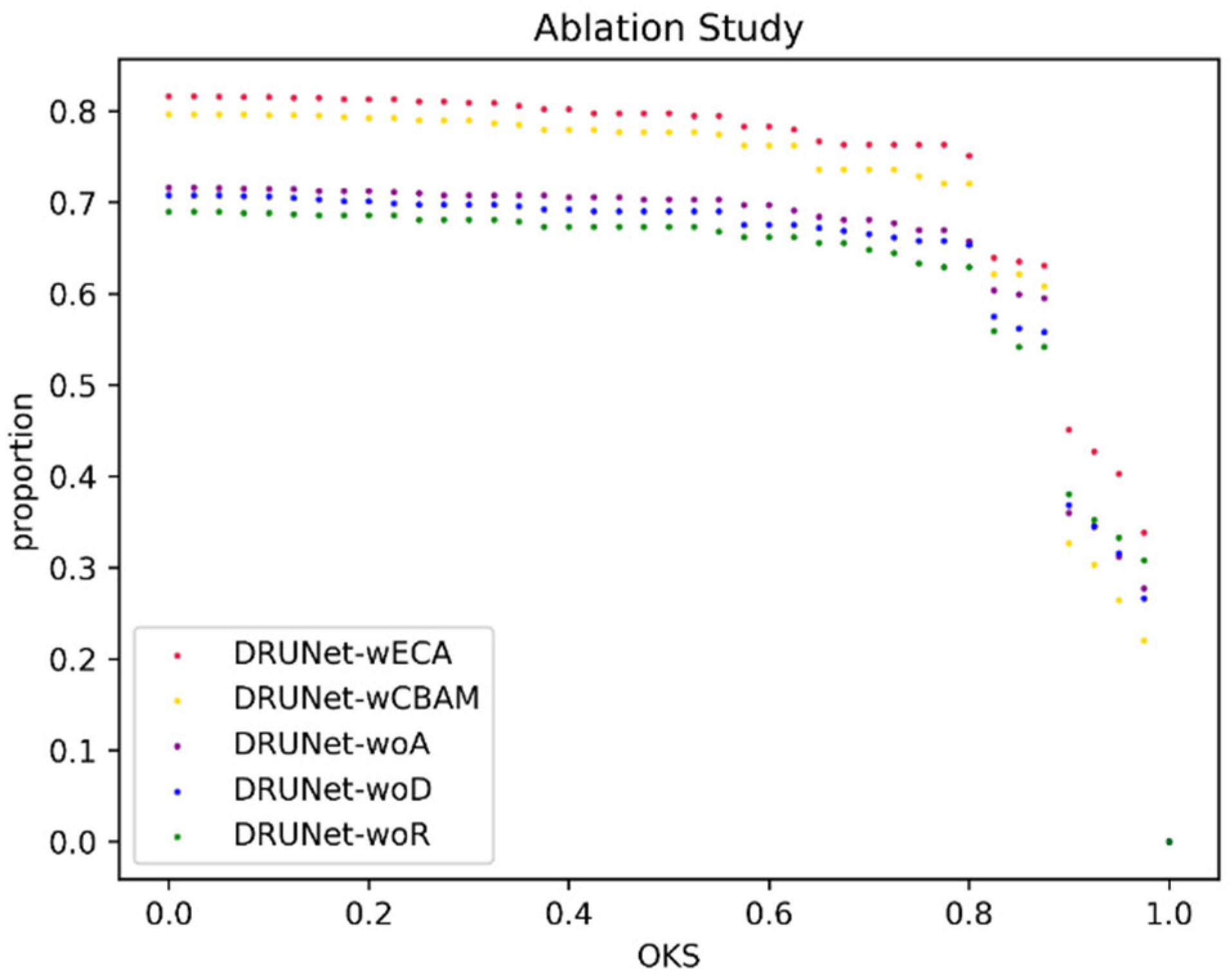
Deep learning network models are usually computed on GPUs, and simply using timing modules in testing would ignore two key issues, resulting in less accurate measured speeds.

In the process of deep learning model inference on GPU, the running process involves two different devices, CPU and GPU, and computational approaches in the field of deep learning are executed asynchronously. Asynchronous execution specifically means that when a function is called by the GPU, it will queue up on the specified device and will not take up other device resources, thus completing parallel computation. This can lead to a timing module running on the CPU needing to choose the right timing method, and there is a possibility that the program on the GPU side has not finished running, but the timing module has already stopped the round of timing, resulting in inaccurate final results. We can solve this problem by switching from asynchronous to synchronous execution of the model on the GPU so that the timing will stop only when the current round of GPU inference is complete.

Another problem is that when the model is deployed on the GPU for inference, the GPU will perform a series of initialization activities, so the GPU needs to be warmed up before the formal time calculation.

The specific metric is the number of frames per second (FPS) that can be processed. The inference speed performance metrics in this paper were made with an RTX3090 24G graphics card, with sufficient intervals for each experiment to ensure that the card was working at its best, feeding the model with a single image size of 256 × 256 and a channel count of 3.

5.3. Ablation Study

To verify the effectiveness of the attentional enhancement module and residual structure we used in each node, we set up several variants as ablation experiments. In the ablation experiment, we propose to verify four questions.

• Question 1: Is the attention enhancement module effective, and how much can it improve performance?
• Question 2: Is the ECA module more suitable than other more complex attention enhancement modules for the detection of weak IR targets?
• Question 3: How much performance optimization can be achieved by using only the residual module for each block without using any attention enhancement module?
• Question 4: Does deep supervision result in improved network performance?

To verify these problems, five experiments were set up, the ablation experiments with the same detection head and all the parameters set in the training process. The difference only lies in the backbone. The specific settings are the same as in the TRAINING METHOD. The results are shown in Figure 7. The horizontal coordinate is the threshold value of OKS in the range of [0, 1], and a total of 40 points are set. The vertical coordinate is the ratio of the number of samples with OKS greater than the threshold to the total number of samples under the current threshold, and the algorithms corresponding to the different results can be seen in the legend. Figure 8 shows an example of Experiment 1 results, and the green dots indicate the positions of the predicted coordinates. As shown in the figure, the green dots can cover the original target.

Table 1. The table shows the results of the ablation experiment, where the threshold indicates the different OKS thresholds, the corresponding value is the proportion of the number of test samples satisfying the threshold to the total number of test samples, and accuracy rate indicates the ratio of the number of test samples with the distance between the predicted coordinates and the real coordinates to the number of test samples with the radius of the inner tangent circle of the target ground truth less than 1.

Experiments	Model	Threshold 0.5	Threshold 0.75	Threshold 0.95	Accuracy Rate	FPS (f/s)	Model Size (MB)
1	DRUNet-wECA	0.7976	0.7633	0.403	0.8247	133	10.5
2	DRUNet-wCBAM	0.7771	0.7286	0.2646	0.8041	53	10.6
3	DRUNet-woA	0.7032	0.6696	0.3121	0.7319	182	10.5
4	DRUNet-woR	0.6735	0.6332	0.3328	0.6907	184	10.5
5	DRUNet-woD	0.6901	0.6577	0.316	0.7268	183	10.5

shows the results of the ablation experimental measurements, and the values representing the best performance are indicated in bolded font. For better quantitative analysis, we extracted three thresholds to create the table, with thresholds of 0.5, 0.75, and 0.95.

The overall trend of Figure 7 shows that our proposed algorithm performs best and has more predicted samples that satisfy the threshold than the other models in the ablation experiment regardless of the OKS threshold. This shows that the network is generally good at the task of predicting the location of the point target. Because of the dense structure and the lightweight ECA attention mechanism, each block in the feature extraction network can share part of the weights, so although the model is relatively deep, the model size is only 10.5 MB and the inference speed is relatively fast.

The comparison of Experiments 1, 2, and 3 can answer question 1. The inclusion of the attention mechanism is effective, and with other quantities held constant, Experiments 1 and 2 have higher accuracy rates of 0.0928 and 0.0722, respectively, than the Experiment 3 accuracy rate without any attention mechanism. OKS scatter plots, on the other hand, visually respond to the greater advantage of Experiments 1 and 2 over the results of Experiment 3.

The comparison of Experiments 1 and 2 answers question 2. Experiment 2 uses the CBAM module [32], which is also seamlessly integrated into any CNN architecture and is more commonly used than the image attention mechanism, which is more complex than the ECA mechanism and is divided into two parts: spatial attention and channel attention, where the feature map input goes first to the channel attention module and then to the spatial attention module, and then the weights obtained from the attention mechanism are multiplied by the input feature map to perform adaptive feature refinement. The DRUNet with the ECA mechanism is 0.0206 higher than the DRUNet with the CBAM mechanism in terms of accuracy rate. The percentage is 0.1384 lower than that of Experiment 1.

This shows that the ECA module is more suitable for the detection of small targets than the CBAM module. Additionally, there is a relatively large difference between the two in terms of inference speed. The model in Experiment 1 has a higher FPS of 80.1783 than the model in Experiment 2. In addition, the model weights in Experiment 1 are slightly smaller than those in Experiment 2 by 0.1 MB.

Regarding problem 3, Experiments 3 and 4 were set up for comparison. The model in Experiment 4, like Experiment 3, uses only the residual structure in each block with deep supervision and without using any special attention mechanism. The scatter plot shows that, overall, the model in Experiment 4 without using the residual structure performs the worst, and it has the lowest percentage in most threshold cases. In addition, the difference in accuracy rate between using and not using the participating residual structure is 0.0412, so there is a benefit of using the residual structure in this small target detection task. There is no difference in model size between the two, and the difference in inference speed is also very small. Therefore, the residual structure is indispensable for model performance improvement, especially in the small target detection task.

The comparison of Experiments 3 and 4 can answer question 4. The accuracy of the former is 0.0051 higher than that of the latter, which is a relatively small difference, but as can be seen from the scatter plot, the models with deep supervision are generally better than those without depth. Models with supervision mechanisms perform better. Therefore, the deep supervision mechanism does bring a performance boost to the model with almost no difference in inference speed.

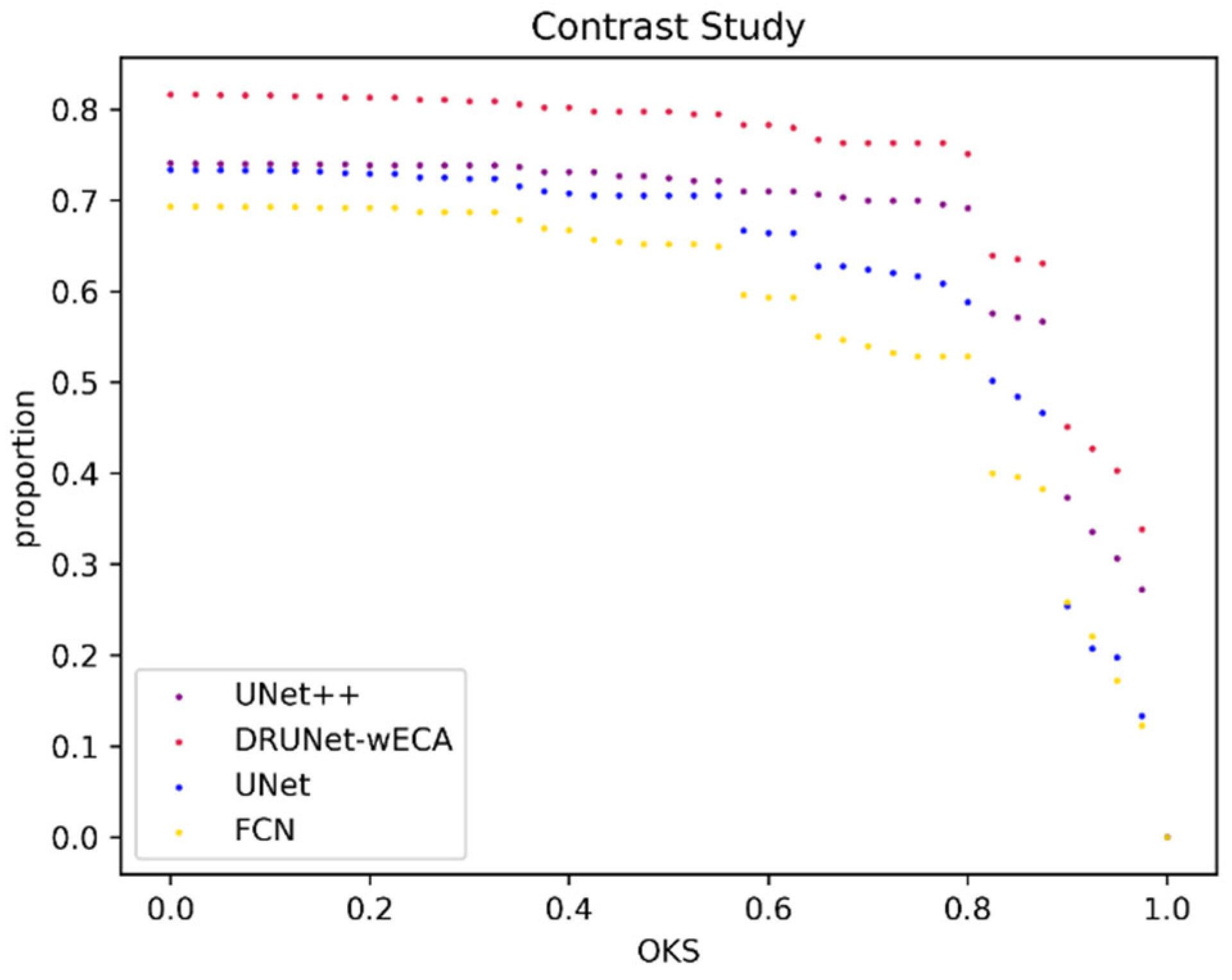
5.4. Contrast Experiment

We selected three feature extraction networks for comparison, and their output feature maps are all the same size as the original input maps. The prediction head uses the same parameters, and the details of the training process are the same as described in the training setup. The results are shown in Figure 9.

As shown in

Table 2. The table shows the results of the constant experiment, where threshold x indicates the different OKS thresholds, the corresponding value is the proportion of the number of test samples satisfying the threshold to the total number of test samples, and accuracy rate indicates the ratio of the number of test samples with the distance between the predicted coordinates and the real coordinates to the number of test samples with the radius of the inner tangent circle of the target ground truth less than 1. FPS indicates the number of images that our experimental platform can process per second, and model size indicates the size of the trained model weights.

Experiments	Model	Threshold 0.5	Threshold 0.75	Threshold 0.95	Accuracy Rate	FPS (f/s)	Model Size (MB)
1	DRUNet-wECA	0.7976	0.7633	0.403	0.8247	133	10.5
2	UNet++	0.7242	0.6995	0.3067	0.7577	146	36.8
3	UNet	0.7054	0.6165	0.1977	0.6855	730	3.2
4	FCN	0.652	0.5285	0.1722	0.5876	327	44.8

, Experiment 1 is our proposed model. The backbone of Experiment 2 is UNET++, and the number of channels varies from shallow to deep 16, 32, 64, 128, and 256, which is consistent with the number of channels per layer variation of DRUNet. The backbone of Experiment 3 is UNet [33], and the biggest difference between UNET and UNet++ is that it only uses long links. Additionally, the overall network shape is simply Experiment 4 uses FCN as the backbone, and FCN [34] is an end-to-end, pixel-to-pixel fully convolutional network for semantic segmentation of images. The overall network structure is divided into two parts: the full convolutional part and the up-sampling part. FCN-32s use the convolutional part of vgg16 as the backbone and change the last three fully connected layers of vgg16 to convolutional layers as well.

Table 2 shows that our proposed algorithm has the best performance, and on the scatter plot, our proposed algorithm keeps leading in terms of the ratio at different thresholds.

Using FCN-32S as the backbone has the worst result, with a difference of 0.2371 from the accuracy rate of our proposed addition algorithm. This is because, in the up-sampling part of FCN-32, it uses a transposed convolution with a step size of 32 to upsample the feature map 32 times, reducing it to the original map size. However, the disadvantage of the FCN-32S model is that the final feature map is upsampled 32 times at once during the up-sampling process, at which time a lot of details are lost during the up-sampling process because the feature map of the last layer is too small. Compared with FCN-32S, UNet performs better because the up-sampling rate of UNet is controlled at 2 times, and the down-sampling rate is controlled at 0.5 times, which is the same setting as our proposed DRUNet. Therefore, for small target detection tasks, the appropriate up-sampling and down-sampling rates are very important, and the sampling rate should not be too large.

The accuracy rate of Experiment 3 is 0.1392 lower than that of Experiment 1, which shows that the dense fusion of shallow and deep features is also crucial for small target detection.

In addition, in terms of speed and model size, the fastest inference time and the smallest model weight is the simplest structure of UNet. However, the detection accuracy of DRUNet is very much higher than that of UNet, and the model weight is also smaller and faster. UNet++ has a faster inference speed than DRUNet with the added ECA attention mechanism and slightly higher accuracy than DRUNet without any added attention mechanism. Therefore, the model structure proposed in this paper is more suitable for the detection of small infrared targets.

6. Conclusions

In this paper, we propose a CNN-based infrared small target detection model, use a dense nested network for feature extraction of small targets in each node, and use an effective attention module ECA and a residual structure to enable the low-level features to be reused and preserve more low-level features for better feature extraction of small targets. We use accuracy rate and simplified OKS to measure the accuracy and validate the inference speed of the model. The experimental results show that the inference speed is slower but acceptable with the best accuracy performance, and the model is only 10.5 MB compared with the base network commonly used in the field of small target detection in complex backgrounds. It can be shown that our proposed feature extraction network is effective for feature extraction of infrared weak targets, and one can try to use this algorithm as a baseline in combination with other applications. We will use it as a baseline for IR small target detection for more improvements and as a backbone for CNN-based IR sequence tracking for more research, such as optimizing it to speed up the inference speed.

References

1. Shi, D.P.; Wu, C.; Li, Z.J.; Pan, W. Research and Progress of Infrared Imaging Technology in the Safety Field. Infrared Technol. 2015, 6, 528–535. [Google Scholar]
2. Zhang, H.; Luo, C.; Wang, Q.; Kitchin, M.; Parmley, A.; Monge-Alvarez, J.; Casaseca-De-La-Higuera, P. A novel infrared video surveillance system using deep learning based techniques. Multimed. Tools Appl. 2018, 77, 26657–26676. [Google Scholar] [CrossRef]
3. Eysa, R.; Hamdulla, A. Issues On Infrared Dim Small Target Detection And Tracking. In Proceedings of the International Conference on Smart Grid and Electrical Automation (ICSGEA), Xiangtan, China, 10–11 August 2019. [Google Scholar]
4. Zhang, W.; Cong, M.; Wang, L. Algorithms for optical weak small targets detection and tracking: Review. In Proceedings of the International Conference on Neural Networks and Signal Processing, Nanjing, China, 14–17 December 2003. [Google Scholar]
5. Liu, Z.; Yang, D.; Li, J.; Hang, C. A review of infrared single-frame dim small target detection algorithms. Laser Infrared 2022, 52, 154–162. [Google Scholar]
6. Zhao, M.; Li, W.; Li, L.; Hu, J.; Ma, P.; Tao, R. Single-Frame Infrared Small-Target Detection. IEEE Geosci. Remote Sens. Mag. 2022, 10, 87–119. [Google Scholar] [CrossRef]
7. Wang, H.X.; Dong, H.; Zhou, Z.Q. Review on Dim Small Target Detection Technologies in Infrared Single Frame Images. Laser Optoelectron. Prog. 2019, 56, 154–162. [Google Scholar]
8. Da Cunha, A.L.; Zhou, J.; Do, M.N. The nonsubsampled contourlet transform: Theory, design, and applications. IEEE Trans. Image Process. 2006, 15, 3089–3101. [Google Scholar] [CrossRef] [PubMed]
9. Comaniciu, D. An algorithm for data-driven bandwidth selection. IEEE Trans. Pattern Anal. Mach. Intell. 2003, 25, 281–288. [Google Scholar] [CrossRef]
10. Buades, A.; Coll, B.; Morel, J.M. A non-local algorithm for image denoising. In Proceedings of the Conference on Computer Vision and Pattern Recognition, San Diego, CA, USA, 20–25 June 2005. [Google Scholar]
11. Hadhoud, M.M.; Thomas, D.W. The two-dimensional adaptive LMS (TDLMS) algorithm. IEEE Trans. Circuits Syst. 1988, 35, 485–494. [Google Scholar] [CrossRef]
12. Chen, C.L.P.; Li, H.; Wei, Y.; Xia, T.; Tang, Y.Y. A Local Contrast Method for Small Infrared Target Detection. IEEE Trans. Geosci. Remote Sens. 2014, 52, 574–581. [Google Scholar] [CrossRef]
13. Qin, Y.; Li, B. Effective Infrared Small Target Detection Utilizing a Novel Local Contrast Method. IEEE Geosci. Remote Sens. Lett. 2016, 13, 1890–1894. [Google Scholar] [CrossRef]
14. Han, J.; Liu, S.; Qin, G.; Zhao, Q.; Zhang, H.; Li, N. A Local Contrast Method Combined With Adaptive Background Estimation for Infrared Small Target Detection. IEEE Geosci. Remote Sens. Lett. 2019, 16, 1442–1446. [Google Scholar] [CrossRef]
15. Davey, S.J.; Rutten, M.G.; Cheung, B. A comparison of detection performance for several track-before-detect algorithms. Eurasip J. Adv. Signal Process. 2007, 2008, 1–10. [Google Scholar] [CrossRef]
16. Zhao, B.; Wang, C.; Fu, Q.; Han, Z. A Novel Pattern for Infrared Small Target Detection With Generative Adversarial Network. IEEE Trans. Geosci. Remote Sens. 2021, 59, 4481–4492. [Google Scholar] [CrossRef]
17. Dai, Y.; Wu, Y.; Zhou, F.; Barnard, K. Asymmetric Contextual Modulation for Infrared Small Target Detection. In Proceedings of the IEEE Winter Conference on Applications of Computer Vision (WACV), Electr Network, Virtual, 5–9 January 2021. [Google Scholar]
18. Dai, Y.; Wu, Y.; Zhou, F.; Barnard, K. Attentional Local Contrast Networks for Infrared Small Target Detection. IEEE Trans. Geosci. Remote Sens. 2021, 59, 9813–9824. [Google Scholar] [CrossRef]
19. Li, B.; Xiao, C.; Wang, L.; Wang, Y.; Lin, Z.; Li, M.; An, W.; Guo, Y. Dense Nested Attention Network for Infrared Small Target Detection. IEEE Trans. Image Process. 2022; Early Access. [Google Scholar] [CrossRef]
20. Zuo, Z.; Tong, X.; Wei, J.; Su, S.; Wu, P.; Guo, R.; Sun, B. AFFPN: Attention Fusion Feature Pyramid Network for Small Infrared Target Detection. Remote Sens. 2022, 14, 3412. [Google Scholar] [CrossRef]
21. Liu, Y.; Liu, H.Y.; Fan, J.L.; Gong, Y.C.; Li, Y.H.; Wang, F.P.; Lu, J. A Survey of Research and Application of Small Object Detection Based on Deep Learning. Acta Electonica Sin. 2020, 48, 590–601. [Google Scholar]
22. Law, H.; Deng, J. CornerNet: Detecting Objects as Paired Keypoints. In Proceedings of the 15th European Conference on Computer Vision (ECCV), Munich, Germany, 8–14 September 2018. [Google Scholar]
23. Law, H.; Teng, Y.; Russakovsky, O.; Deng, J. CornerNet-Lite: Efficient Keypoint Based Object Detection. arXiv 2019, arXiv:1904.08900. [Google Scholar]
24. Zhou, X.; Zhuo, J.; Krahenbuhl, P. Bottom-up Object Detection by Grouping Extreme and Center Points. In Proceedings of the 32nd IEEE/CVF Conference on Computer Vision and Pattern Recognition (CVPR), Long Beach, CA, USA, 16–20 June 2019. [Google Scholar]
25. Zhou, X.; Wang, D.; Krähenbühl, P. Objects as Points. arXiv 2019, arXiv:1904.07850. [Google Scholar]
26. Li, Y.; Chen, Y.; Wang, N.; Zhang, Z. Scale-Aware Trident Networks for Object Detection. In Proceedings of the IEEE/CVF International Conference on Computer Vision (ICCV), Seoul, Korea, 27 October–2 November 2019. [Google Scholar]
27. Zhou, Z.; Rahman Siddiquee, M.M.; Tajbakhsh, N.; Liang, J. UNet plus plus: A Nested U-Net Architecture for Medical Image Segmentation. In Proceedings of the 4th International Workshop on Deep Learning in Medical Image Analysis (DLMIA)/8th International Workshop on Multimodal Learning for Clinical Decision Support (ML-CDS), Granada, Spain, 20 September 2018. [Google Scholar]
28. Wang, Q.; Wu, B.; Zhu, P.; Li, P.; Zuo, W.; Hu, Q. ECA-Net: Efficient Channel Attention for Deep Convolutional Neural Networks. arXiv 2019, arXiv:1910.03151. [Google Scholar]
29. Huang, G.; Liu, Z.; Van Der Maaten, L.; Weinberger, K.Q. Densely Connected Convolutional Networks. In Proceedings of the 30th IEEE/CVF Conference on Computer Vision and Pattern Recognition (CVPR), Honolulu, HI, USA, 21–26 July 2017. [Google Scholar]
30. Wang, H.; Zhou, L.; Wang, L. Miss Detection vs. False Alarm: Adversarial Learning for Small Object Segmentation in Infrared Images. In Proceedings of the IEEE/CVF International Conference on Computer Vision (ICCV), Seoul, Korea, 27 October–2 November 2019.
31. Hui, B.W.; Song, Z.Y.; Fan, H.Q.; Zhong, P.; Hu, W.D.; Zhang, X.F.; Ling, J.G.; Su, H.Y.; Jin, W.; Zhang, Y.J.; et al. A dataset for dim-small target detection and tracking of aircraft in infrared image sequences [DB/OL]. Sci. Data Bank 2019. under review. [Google Scholar] [CrossRef]
32. Woo, S.; Park, J.; Lee, J.Y.; Kweon, I.S. CBAM: Convolutional Block Attention Module. In Proceedings of the 15th European Conference on Computer Vision (ECCV), Munich, Germany, 8–14 September 2018. [Google Scholar]
33. Ronneberger, O.; Fischer, P.; Brox, T. U-Net: Convolutional Networks for Biomedical Image Segmentation. In Proceedings of the 18th International Conference on Medical Image Computing and Computer-Assisted Intervention (MICCAI), Munich, Germany, 5–9 October 2015. [Google Scholar]
34. Long, J.; Shelhamer, E.; Darrell, T. Fully Convolutional Networks for Semantic Segmentation. IEEE Trans. Pattern Anal. Mach. Intell. 2017, 39, 640–651. [Google Scholar]
Figure 1. The structure of DRUNet is shown in the figure. The image of arbitrary size W × H × C is reshaped to 256 × 256 × 3 and input to the backbone network for feature extraction, becoming a feature map of the size 256 × 256 × 1. Finally, the target center point coordinates are output through the prediction head.
Applsci 12 09299 g001
Figure 2. This is a diagram of our efficient channel attention (ECA) module. Using aggregated features generated by global average pooling (GAP), ECA generates channel weights by performing a fast 1D convolution of size k, where k is adaptively determined based on channel dimension C.
Applsci 12 09299 g002
Figure 3. The structure of the ECA-Rest Block is shown in the figure. The input of each block is summed with the original input after a 2D convolution, BatchNorm, and ECA module, and after a ReLU activation layer, we can take the output of this block.
Applsci 12 09299 g003
Figure 4. The figure shows a schematic diagram of DRUNet; each node is ECA-Rest Block. The legend on the top right indicates the operations of the different shapes and colors of lines in the structure graph, and the legend on the bottom right indicates the functions and parameters corresponding to these operations. The operations of skip connect and connect are both cat, linking the feature map in the first dimension of the feature map; for example, the shape of feature map A is (batch size, channels_1,H,W), the shape of B is (batch size, channels_2,H,W), and the size of the feature map after connection is (batch size, channels_1+channels_2,H,W).
Applsci 12 09299 g004
Figure 5. The arrow points to a magnified image of the small target, from which it can be seen that the center point of the small target is not easily defined.
Applsci 12 09299 g005
Figure 6. These six images are from the dataset used in this experiment, and the targets are pointlike and not the brightest area in the image, with a complex background. Not only images (a,d,e) contain one bright spot, but also it is difficult to identify which bright spot is the real target by directly observing a single frame of the image, making the detection task more challenging. The background of images (b,c,f) is not as complex but the target is also small and weak.
Applsci 12 09299 g006
Figure 7. The figure shows the OKS scatter plot of the ablation experiment, with the horizontal coordinate showing the different OKS thresholds and the vertical coordinate showing the proportion of test samples meeting the current OKS threshold to the total test samples.
Applsci 12 09299 g007
Figure 8. These pictures show the effect of the predicted coordinate tracing points, and it can be seen that the offset of the network prediction results is small and can overlap with the small target. Figure (a) is from the SIRST dataset, and its size is less than 256 × 256. To not change the size of the small target in the picture, it is changed to 256 × 256 by padding. Figure (bd) from ground/air background infrared image small aircraft target detection tracking dataset.
Applsci 12 09299 g008
Figure 9. The figure shows the OKS scatter plot of the constant experiment, with the horizontal coordinate showing the different OKS thresholds and the vertical coordinate showing the proportion of test samples meeting the current OKS threshold to the total test samples. FPS indicates the number of images that our experimental platform can process per second, and model size indicates the size of the trained model weights.
Applsci 12 09299 g009