Cognitive Artificial Intelligence Using Bayesian Computing Based on Hybrid Monte Carlo Algorithm

Abstract

Cognitive artificial intelligence (CAI) is an intelligent machine that thinks and behaves similar to humans. CAI also has an ability to mimic human emotions. With the development of AI in various fields, the interest and demand for CAI are continuously increasing. Most of the current AI research focuses on the realization of intelligence that can make optimal decisions. Existing AI studies have not conducted in-depth research on human emotions and cognitive perspectives. However, in the future, the demand for the use of AI that can imitate human emotions in various fields, such as healthcare and education, will continue. Therefore, we propose a method to build CAI in this paper. We also use Bayesian inference and computing based on the hybrid Monte Carlo algorithm for CAI development. To show how the proposed method for CAI can be applied to practical problems, we create an experiment using simulation data.

1. Introduction

From symbolic and connectionist paradigms to present-day deep learning methods, various studies of artificial intelligence (AI) have been conducted [1,2,3]. In the meantime, not only computer science, but also mathematics, statistics, brain science, psychology, and industrial engineering have been interdisciplinary studies for AI research [4,5,6]. To date, most AI research has aimed at developing intelligent systems that perform optimal decision-making procedures. For example, AI playing Go focused on the goal of defeating opponents [7]. However, when humans play the Go game, in some cases, they perform actions that are slightly advantageous to their opponents for the fun of the game. We have to consider other concepts of current AI technology. Therefore, we propose cognitive AI (CAI) in our research. CAI is AI that imitates human thinking and behaves with emotion [8]. As the research on AI in various fields is more actively conducted, the demand for CAI will increase further [8,9]. For instance, in the fields of healthcare and education, the need for CAI that can emotionally communicate with humans has been raised [10,11,12,13,14]. The research on CAI is still at an early stage. Sumari and Syamsiana (2021) presented an introduction to a knowledge-growing system by CAI [6]. In addition, Sumari et al. (2021) proposed predictions using a knowledge-growing system as a CAI approach [15]. The previous two studies related to CAI focused on knowledge-growing systems and did not deal with human decision making based on emotions. In another study related to CAI, Jun (2021) proposed a method for making a machine capable of mimicking human thinking [8]. The method applied the results of a posterior distribution and Bayesian bootstrap to construct a machine imitating human thinking [8]. In this paper, we also use a method for CAI development using advanced Bayesian computing. We consider the hybrid Monte Carlo (HMC) algorithm for our Bayesian approach [16,17,18,19,20,21,22,23]. Human thinking is performed through fast computation based on a parallel neural network structure. Therefore, we chose HMC, which has a faster computation speed than the popular Metropolis–Hastings algorithm in Bayesian learning [16,17,18]. The HMC algorithm is used to construct model parameters [19,20,21,22,23]. This paper contributes to developing machines that think and behavior similar to humans with emotion. We apply the HMC algorithm to create the proposed method. We expect our research results to be used in the development of human-friendly AI systems in various practical applications, such as healthcare, education, and mobility. Traditional AI focuses on optimal decision making, but the CAI proposed in this study focuses on the development of machines that mimic human emotions.

In order to proceed with the proposed research, we organized our paper as follows. In Section 2, the research background is introduced. In this section, we describe the concepts of cognitive systems for AI and Markov Chain Monte Carlo (MCMC) algorithms. We present our proposed method for CAI in Section 3. In the next section, we perform a simulation study to show how the proposed method can be used in real domains. Lastly, we present our conclusions and future works in Section 5.

2. Research Backgrounds

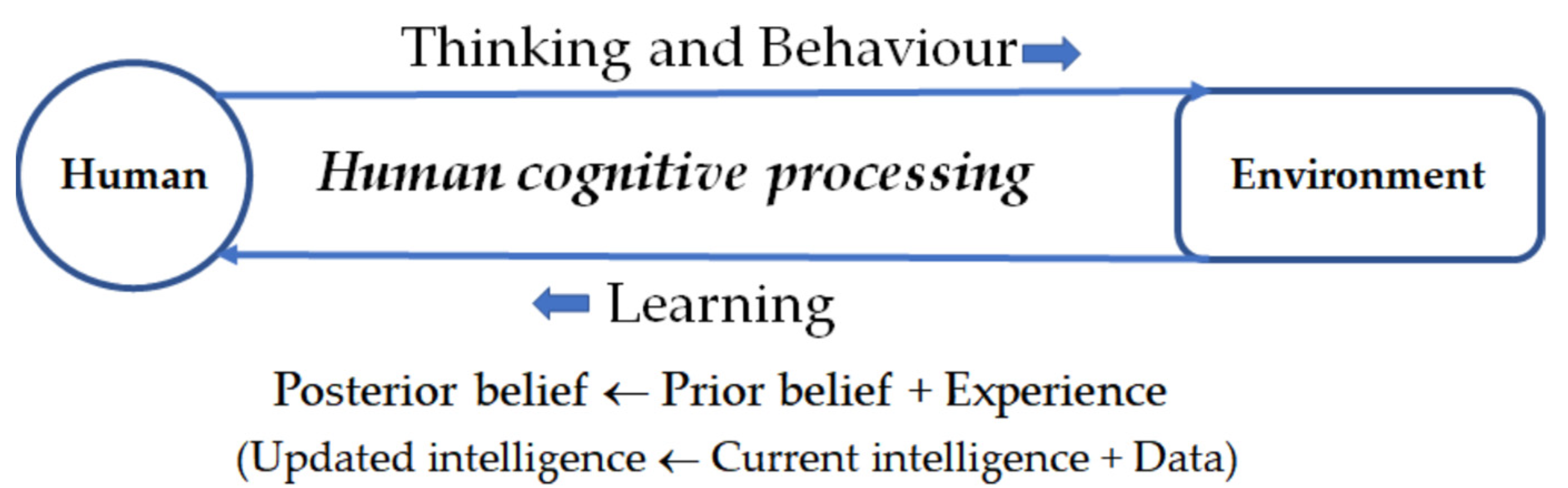
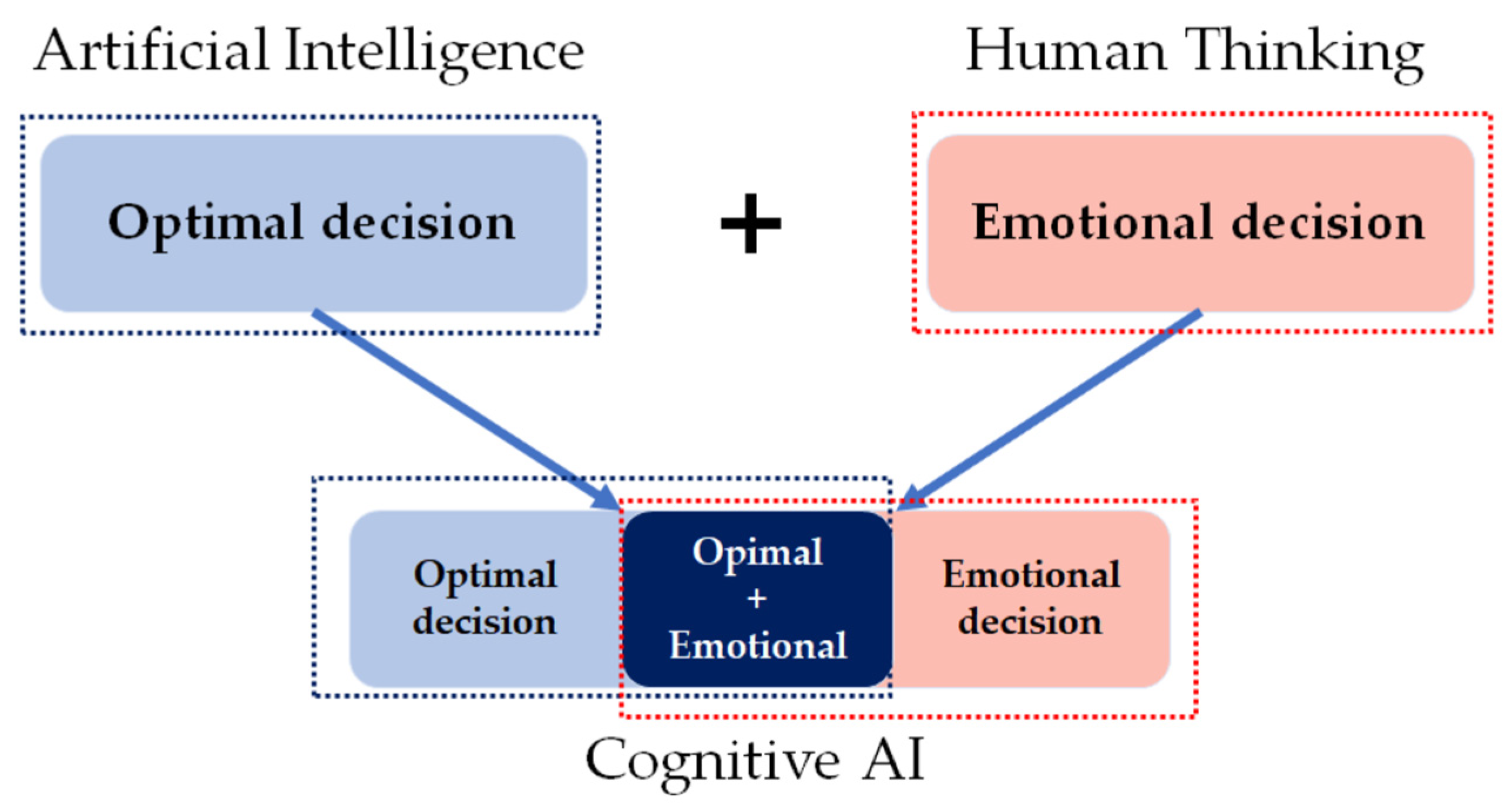
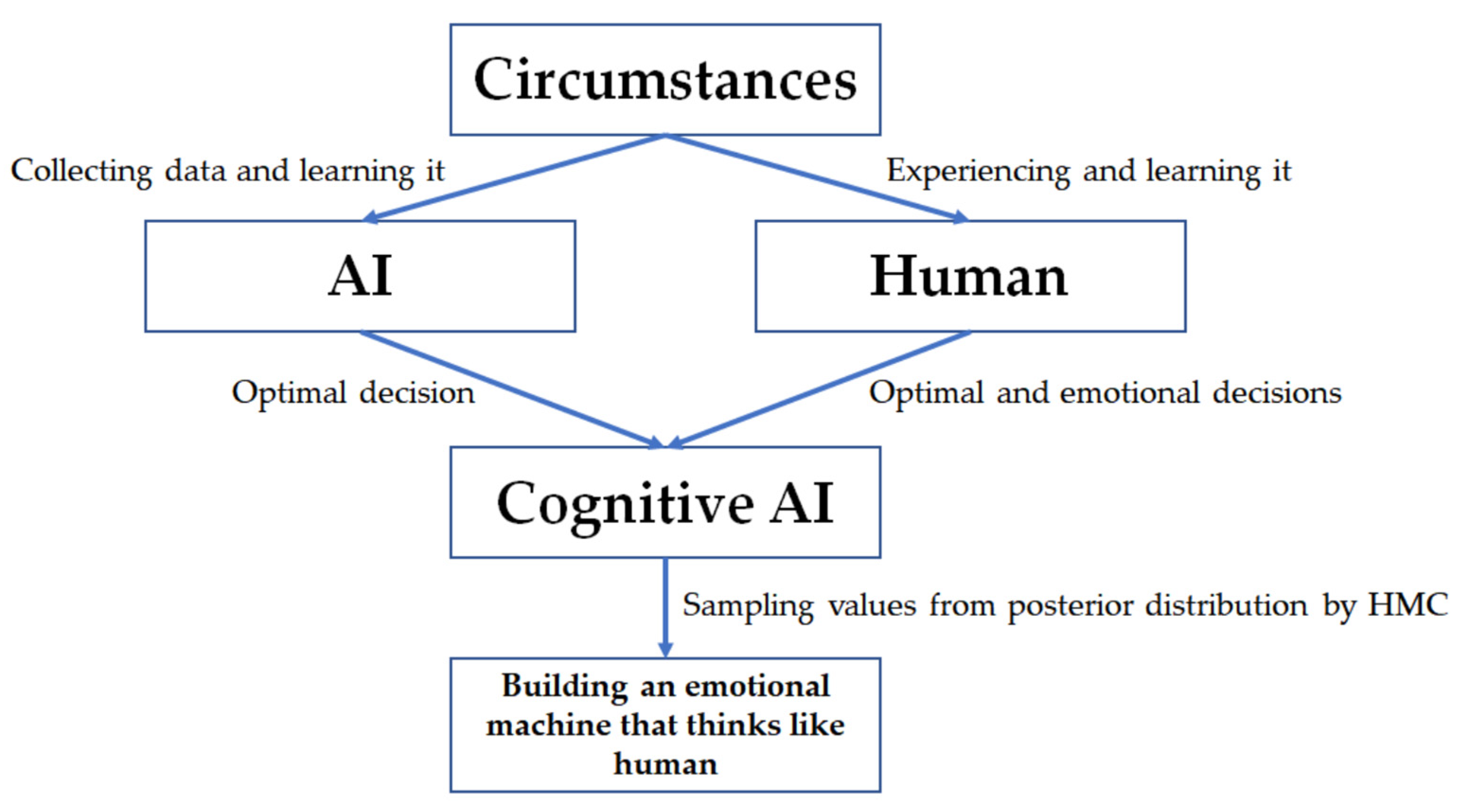
2.1. Cognitive Systems for Artificial Intelligence

At present, most research conducted on AI is to develop intelligence to make optimal decisions [2,24,25,26,27]. The goal of AI is to find the optimal solution to a given problem [2,24,27]. In contrast, humans do not always make optimal decisions [8,28]. Sometimes, humans make decisions based on emotions [28]. CAI is an AI that imitates human thinking and behavior by emotion as well as optimization [8]. Jun (2021) studied Bayesian learning and bootstrapping to develop machines imitating human thinking [8]. This research used prior and data and combined the posterior and Bayesian bootstrap intervals [8]. It is very difficult to create machines that think and behave similar to humans [5]. This is because it is difficult for machines to have a human-like cognitive ability with the current technology. Therefore, we studied the building of CAI with cognitive abilities similar to humans using Bayesian computing based on HMC.

To date, the research on CAI has been largely developed based on two academic fields. The first is the field of computer science, including data science and statistics. The second is cognitive science, including psychology.

Table 1. Existing research results of optimal and emotional AI according to computer and cognitive sciences.

CAI	Optimal AI	Emotional AI
Computer science Data science Statistics	Silver et al. (2016) [7] Russell and Norvig (2014) [2] Goodfellow et al. (2016) [3] Neal (1996) [17] Ghahramani (2015) [31]	Sumari and Syamsiana (2021) [6] Jun (2021) [8]
Cognitive science Psychology Cognitive psychology	Griffiths et al. (2012) [32] Mnih et al. (2015) [34] Tenenbaum et al. (2011) [35] Ellis et al. (2022) [36] Krafft et al. (2021) [38]	Lake et al. (2017) [5] Economides et al. (2015) [29] Gershman et al. (2015) [30] Lake et al. (2015) [33] Kryven et al. (2021) [37]

shows the existing research results of optimal and emotional AI according to computer and cognitive sciences [2,3,5,6,7,8,29,30,31,32,33,34,35,36,37,38].

In the field of cognitive science, including psychology and cognitive psychology, both studies of optimal and emotional AI systems have been actively progressing. On the other hand, in computer science, including data science and statistics, the research on optimal AI has progressed to a high level, but the research on emotional AI has not yet been properly conducted. Sumari and Syamsiana (2021) [6] studied the CAI for knowledge-growing system rather than the development of AI that mimics human thoughts and emotions. Therefore, we confirmed the need for research on emotional AI from the point of view of computer science.

2.2. Markov Chain Monte Carlo Algorithms

The goal of Bayesian inference is to construct a posterior distribution and parameter θ [39,40,41]. The posterior distribution is built by combining the prior of θ and likelihood [39,42]. When a model is complicated or the number of parameters increases, it becomes difficult for us to accurately obtain the posterior distribution [43]. Therefore, we considered the Markov Chain Monte Carlo (MCMC) algorithms to estimate the posterior distribution of θ. We have to obtain the posterior sample to estimate θ. There are various MCMC methods, such as Gibbs sampler and the Metropolis–Hastings algorithm. Among them, the Metropolis–Hastings algorithm has been used in Bayesian computing. This is performed by the following steps [39,43]:

• (Step 1) Drawing initial value ${\theta }_0$ from starting distribution $p_0\left(\theta \right)$.
• (Step 2) Sampling new parameter value ${\theta }_i$ from proposal distribution ($i=1,2,\dots$).
• (Step 3) Calculating the acceptance probability of the new parameter value by (1).

  $$p_{acceptance}\left({\theta }_{i+1}|{\theta }_i\right)=min\left(1,\frac{p\left({\theta }_{i+1}\right)q({\theta }_i|{\theta }_{i+1})}{p\left({\theta }_i\right)q({\theta }_{i+1}|{\theta }_i)}\right)$$

  (1)
• (Step 4) Selecting a new parameter value if the acceptance probability is higher than the value obtained from a uniform distribution on [0, 1]; otherwise, it stays at the current value.
• (Step 5) Repeating Steps 2 through 4 until we have enough samples.

We drew an initial value for start parameter ${\theta }_0$ in Step 1. Subsequently, we sampled a new parameter value ${\theta }_i$ at time period i, ($i=1,2,\dots$) in Step 2. In Step 3, the Metropolis–Hastings criteria to accept a new parameter value was shown. If the probability of $p_{acceptance}\left({\theta }_{i+1}|{\theta }_i\right)$ was larger than the random value generated from a uniform distribution of [0, 1], we accepted the new value (${\theta }_{i+1}$); otherwise, we selected current parameter value (${\theta }_i$). In general, the MCMC methods, including the Metropolis–Hastings algorithm, required enough samples for an accurate approximation of the posterior distribution. Moreover, the methods needed a long computation time. To overcome the problems, we applied the HMC algorithm to our CAI model.

3. Proposed Method

In this paper, we proposed a method to build CAI, a learning machine that can mimic human thoughts and emotions. We introduced the cognitive processing of humans interacting with the surrounding environment in Figure 1.

Humans improve their current knowledge by absorbing the considerable amount of data they experience from their surroundings. That is, humans combine their current knowledge with data, and update the intelligence by learning from data. The current and updated knowledge represent the prior and posterior distributions in Bayesian learning. Therefore, humans learn from the data experienced in the environments and improve their intelligence by the results of learning from data, based on the updated intelligence every time humans think about and behave according to their surroundings. In human cognitive processing, humans do not always make optimal decisions. Sometimes, they present emotional thinking and behavior. This is the greatest difference between the CAI proposed in this paper and the existing AI. Figure 2 presents our CAI structure combining AI and human thinking.

At present, the aim of AI is to develop an intelligent machine for optimal decision making. In contrast, humans make decisions and actions that are biased by emotions, as well as optimal decision making. In Figure 2, the CAI works by combining the functions of optimal and emotional decisions in AI and humans. Therefore, we proposed a method to develop CAI performing optimal and emotional behaviors similar to humans. In this paper, we considered Bayesian learning to construct our CAI, because the Bayesian learning process is similar to humans learning from surrounding environments [5,17,40]. Bayesian learning is performed by prior distribution, likelihood function, and posterior distribution [40]. The prior distribution represents the current belief in each task. The likelihood function figures out the experience under prior knowledge. That is, the function explains the results observing the data in environments. Lastly, we have the posterior distribution, which is the updated belief of the task. This distribution is obtained by multiplying the prior distribution and likelihood function. In reality, it is difficult for us to accurately obtain the posterior distribution because the model is complex or there are many parameters to estimate [16]. Therefore, we used MCMC methods to approximately estimate the posterior distribution. The Gibbs sampler and Metropolis–Hastings algorithm are popular MCMC methods. However, they are not suitable for modeling human thinking and behavior because they require a lengthy computation time and many samples. That is, the Metropolis–Hastings algorithm requires enough samples to obtain accurate approximation of the target distribution [41]. Therefore, we needed a lot of time to obtain enough samples. Since the computation time is important in CAI that mimics the rapid human thought process, it is difficult to obtain a sufficient sample because it takes a lot of time. To solve this problem, we considered HMC as a more efficient method for MCMC. HMC provides better results in high-dimensional and complex modeling compared to the existing methods, such as Gibbs sampling or the Metropolis–Hastings algorithm in MCMC [16]. In general, human thinking is multidimensional and complex; therefore, in this paper, we proposed a CAI method using HMC. HMC is also one of the MCMC methods used for Bayesian inference. In the current paper, we proposed a method of Bayesian computing using HMC for constructing CAI.

HMC produces better performance than the Metropolis–Hastings algorithm because it can avoid random walk behavior [17]. Furthermore, this is an algorithm combining the Metropolis algorithm and sampling method by dynamical simulations [17]. We obtained a sample of points extracted from a specified distribution as a result of HMC. Therefore, HMC accepts the proposals at a much higher rate than the Metropolis–Hastings algorithm. In the HMC algorithm, the horizontal and vertical locations are represented by θ and q, where θ is the parameter estimated by the HMC chain and q is a parameter for the momentum of the HMC procedure. Moreover, θ follows the posterior distribution $f\left(\theta \right)$ and q is used to simulate θ in the following formula called the Hamiltonian equation [16,17].

$$H\left(\theta ,q\right)=P\left(\theta \right)+K\left(q\right)$$

(2)

where the Hamiltonian function $H\left(\theta ,q\right)$ consists of energy functions $P\left(\theta \right)$ and $K\left(q\right)$ for potential and kinetic energies. As with other MCMC methods, we sampled θ from $f\left(\theta \right)$. The $P\left(\theta \right)$ represents $-logf\left(\theta \right)$ and q follows normal distribution $N_k\left(0,\mathsf{\Sigma }\right)$, where k is the vector length of θ and $\mathsf{\Sigma }$ is the given variance–covariance matrix. Therefore, Equation (2) is expressed as follows [16,44]:

$$H\left(\theta ,q\right)=-logf\left(\theta \right)+\frac{1}{2}{q}^T{\mathsf{\Sigma }}^{-1}q$$

(3)

By first differentiating Equation (3) with respect to time t, we solve the Hamiltonian differential equations in HMC. So, we show the HMC algorithm precedure as follows.

• (Step 1) Initializing

  (1-1)

  Initial value of parameters, ${\theta }^0$;

  (1-2)

  Time start, t = 1;

  (1-3)

  Initial log posterior density, $logf\left({\theta }^0\right)$;

  (1-4)

  Generating momentum q from $N\left(0,\mathsf{\Sigma }\right)$.

• (Step 2) Sampling

  (2-1)

  Starting states for leapfrog, $\tilde{\theta }={\theta }^{t-1}, \tilde{q}=q$;

  (2-2)

  Repeating leapfrog algorithm (L times);

  (2-3)

  Producing HMC proposal density, $\tilde{\theta }$ and $\tilde{q}$.

• (Step 3) Accepting or rejecting

  (3-1)

  Determining acceptance probability, α;

  (3-2)

  If accepting, ${\theta }^t=\tilde{\theta }, q^t=-\tilde{q}$;

  (3-3)

  If rejecting, ${\theta }^t={\theta }^{t-1}, q^t=q^{t-1}$.

• (Step 4) Repeating Steps 2 and 3 until N samples are obtained, $t=t+1$.

In Step 3, the acceptance probability α is determined by (4) [16].

$$\mathsf{\alpha }=\min \left(1,\frac{exp\left(logf\left(\tilde{\theta }\right)-\frac{1}{2}{\tilde{q}}^T{\mathsf{\Sigma }}^{-1}\tilde{q}\right)}{exp\left(logf\left({\tilde{\theta }}^{t-1}\right)-\frac{1}{2}{q}^T{\mathsf{\Sigma }}^{-1}q\right)}\right)$$

(4)

In the current paper, we focused on the regression analysis for target modeling in CAI. Therefore, we consider the regression model as follows:

$$y={\beta }_0+{\beta }_1{X}_1+{\beta }_2{X}_2+\cdots +{\beta }_p{X}_p+e$$

(5)

In (5), $X=\left(1,X_1,X_2,\dots ,X_p\right)$ is the explanatory variable vector and $y$ is the response variable. The first element of $X$, 1 is a value corresponding to intercept ${\beta }_0$. The e value is an error term following the Gaussian distribution with mean zero and constant variance ${\sigma }_e^2$. $\beta =\left({\beta }_0,{\beta }_1,\dots ,{\beta }_p\right)$ is the parameter vector corresponding to $X$. The likelihood function is expressed as Equation (6) [43]:

$$f\left(y|\beta ,{\sigma }_e^2\right)={\left(\frac{1}{\sqrt{2\pi }{\sigma }_e}\right)}^{n}exp\left(-\frac{1}{2{\sigma }_e^2}{\left(y-X\beta \right)}^T\left(y-X\beta \right)\right)$$

(6)

where n is the number of data elements. Subsequently, the priors of $\beta$ and e are the following distributions of (7) and (8):

$$\beta ~\mathrm{N}\left({\mu }_{\beta },{\mathsf{\Sigma }}_{\beta }\right)$$

(7)

$${\sigma }_e^2~Inverse-gamma\left(a,b\right)$$

(8)

By multiplying the priors and likelihood function, we obtain the posterior distribution as (9) [43]:

$$\mathrm{F}\left(\beta ,{\sigma }_e^2|y\right)\propto f\left(y|\beta ,{\sigma }_e^2\right)exp\left(-\frac{1}{2}{\left(\beta -{\mu }_{\beta }\right)}^T{\mathsf{\Sigma }}_{\beta }^{-1}\left(\beta -{\mu }_{\beta }\right)\right){\left({\sigma }_e^2\right)}^{-a-1}{e}^{-\frac{b}{a^2}}$$

(9)

Using HMC based on (6)–(8), the regression parameters $\widehat{\beta }=\left({\widehat{\beta }}_0,{\widehat{\beta }}_1,\dots ,{\widehat{\beta }}_p\right)$ are estimated. When the new input $X^{new}$ is given, we predict response $y$ using the estimated parameters and $X^{new}$. In this case, the prediction of $y$ is always an optimal single value. However, the CAI does not predict single value $y$ given $X^{new}$, it predicts various values as well as optimal values by its thinking and emotion. To overcome this problem, we estimate confidence intervals of regression parameters as (10) [43]:

$$CI\left({\beta }_i,1-\alpha \right)=\left({\widehat{\beta }}_i-t_{\alpha /2}\frac{{\sigma }_e}{\sqrt{n}},{\widehat{\beta }}_i+t_{\alpha /2}\frac{{\sigma }_e}{\sqrt{n}} \right), i=0,1,2,\dots ,p$$

(10)

where $\alpha$ is the significance level and has a value between 0 and 1. For example, we obtain a 90% confidence interval when $\alpha$ is 0.5. As the value of $\alpha$ increases, the length of the confidence interval decreases. In the current paper, we applied the lower and upper bounds of confidence intervals for the parameters of the uniform distribution. To derive CAI decisions, we sampled the random number from the uniform distribution and used this value as the regression parameter. Therefore, we could predict a different response $y$ each time for the same given $X$. Moreover, we could control the degree of emotion according to $\left(1-\alpha \right)$. As this value increased, the length of the confidence interval increased and the emotional degree increased, so that it was possible to provide various predicted values for y. Figure 3 illustrates the flowchart for our proposed method.

In Figure 3, AI and humans all collect experience and data from external circumstances. The experienced data is learned by AI and humans. Through this process, AI performs optimal decision making, and humans not only make optimal decisions but also act based on their emotions. This is the CAI proposed in this paper. Finally, we used HMC to build an emotional machine that can think emotionally similar to humans. Subsequently, we showed the performance and validity of our method by a simulation study.

4. Experiments and Results

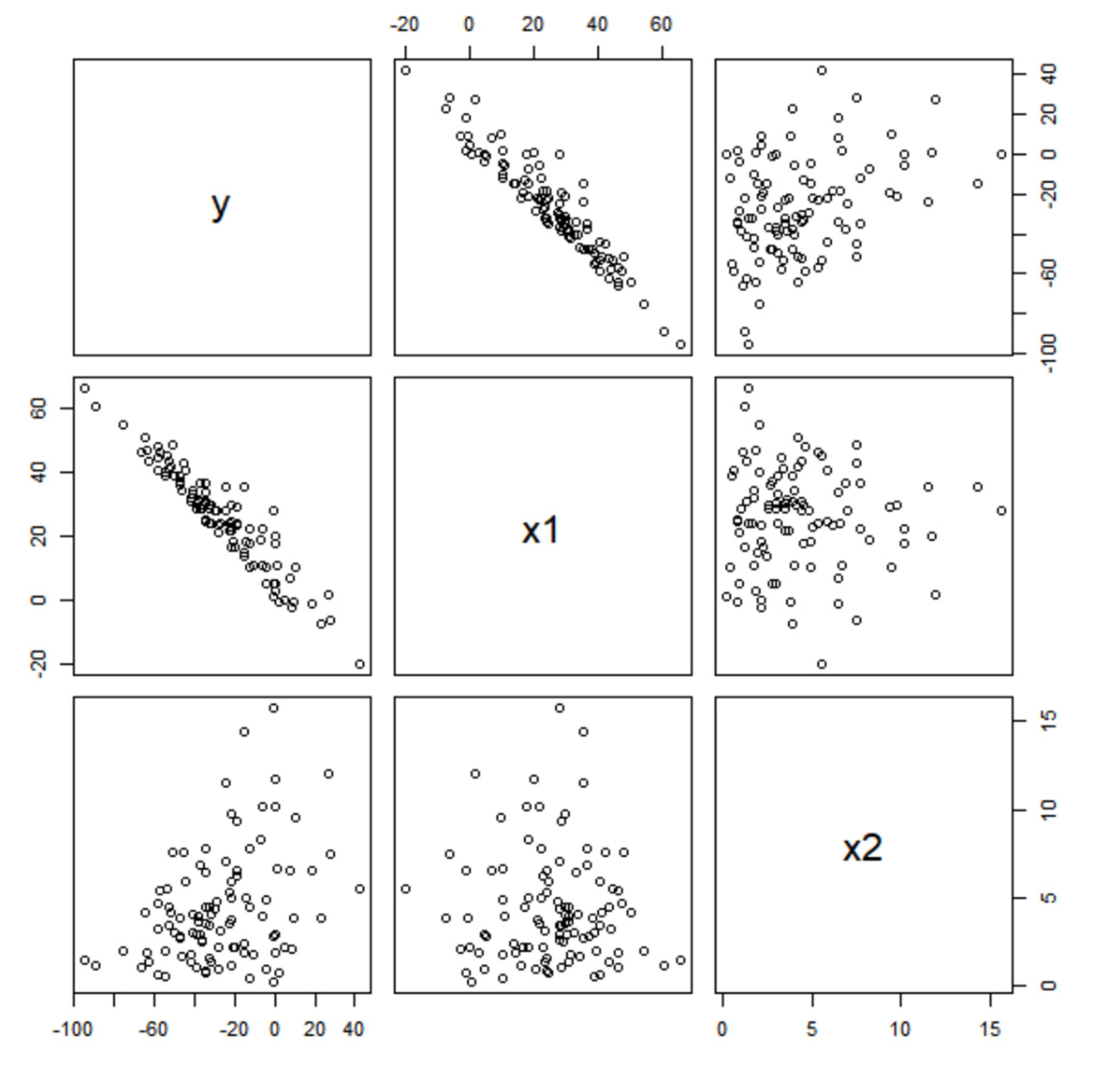
4.1. Simulation Data

To illustrate how our proposed method can be applied to practical cases, we used simulated data and designed the following regression model:

$$\mathrm{Y}=0.5-1.5X_1+2.5X_2+e$$

(11)

In (11), $X_1$ and $X_2$ are explanatory variables and Y is the response variable. Moreover, e is the error term. In general regression models, Y and e are random variables with probability distributions. In order to conduct our experiments, we generated simulation data with $X_1$, $X_2,$ and e by the probability distributions presented in

Table 2. Probability distributions for generating simulation data.

Variable	Distribution	Parameter	Expectation	Variance
$X_1$	Gaussian	Mean = 24 Standard deviation = 16	$E\left(X_1\right)=24$	$Var\left(X_1\right)={16}^2$
$X_2$	Gamma	Shape = 2 Inverse scale = 0.5	$E\left(X_2\right)=$4	$Var\left(X_2\right)=8$
$e$	Gaussian	Mean = 0 Standard deviation = 1	$E\left(e\right)=0$	$Var\left(e\right)=1$

.

We determined the Gaussian and gamma distributions for $X_1$ and $X_2$, respectively. In Table 1, the density function is shown in (12) [42]:

$$\mathrm{f}\left(x_1|\mu =24,\sigma =16\right)=\frac{1}{\sqrt{2\pi }\sigma }exp\left(-\frac{{\left(x_1-\mu \right)}^2}{2{\sigma }^2}\right),-\infty <x_1<\infty$$

(12)

Therefore, $X_1$ has values ranging from negative infinity to positive infinity. As in the following Equation (13), $X_2$ has a real value greater than 0 [42]:

$$\mathrm{f}\left(x_2|\alpha =2,\beta =0.5\right)=\frac{{\beta }^{\alpha }}{\mathsf{\Gamma }\left(\alpha \right)}{x}_2^{\alpha -1}exp\left(\beta x_2\right), x_2>0$$

(13)

where $\alpha$ and $\beta$ are the shape and inverse scale parameters of the gamma probability density. In addition, $\mathsf{\Gamma }\left(\alpha \right)$ is the gamma function of $\alpha$ [42]. The error term e also follows the same Gaussian distribution as $X_1$, and the mean and standard deviation of the distribution are 0 and 1, respectively. Therefore, we generated the simulation data for $X_1$, $X_2$, and e using the probability densities presented in Table 2. Figure 4 illustrates the scatter plots between the variables simulated in Table 2.

We knew that $\mathrm{Y}$ and $X_1$ were strongly negatively correlated with each other and $\mathrm{Y}$ and $X_2$ were weakly positively correlated. The error term e was used as noise following the standard normal distribution. Using the simulation data, we performed regression analysis and present the results of the comparative methods in

Table 3. Estimated parameters and intervals: simulation data.

	Estimated		Confidence Interval: HMC
	GLM	HMC	50%	90%
${\beta }_0$	0.1987	0.6866	(0.6866, 0.6866)	(0.6866, 1.0489)
${\beta }_1$	−1.4923	−1.4878	(−1.4971, −1.4878)	(−3.6898, −1.4878)
${\beta }_2$	2.5389	2.4011	(2.4011, 2.4011)	(1.7923, 2.5970)

.

Table 3 represents the results of the parameter estimation. In this table, we compared HMC with a generalized linear model (GLM) based on least squares. The values of the estimated parameters are presented in the first column. We observed that the ${\beta }_0$ values of GLM and HMC were different from each other. On the other hand, we observed that the ${\beta }_1$ and ${\beta }_2$ values were estimated to be similar to each other in GLM and HMC. We also presented the confidence intervals of the parameters estimated by HMC. In Table 3, we computed two confidence intervals according to the significance levels of 50% and 90% for the parameters of ${\beta }_0$, ${\beta }_1$, and ${\beta }_2$. We observed that the length of the confidence interval with a significance level of 90% was greater than 50%. Subsequently, in

Table 4. Optimal and emotional decisions: simulation data.

Input		Optimal		Emotional: HMC
${\mathit{X}}_{\mathbf{1}}$	${\mathit{X}}_{\mathbf{2}}$	GLM	HMC	0.5	0.9
2	2 4 6	2.2919 7.3697 12.4475	2.5132 7.3154 12.1176	(2.4987, 2.4989, 2.5021) (7.3009, 7.3011, 7.3043) (12.1031, 12.1033, 12.1065)	(2.1376, −0.3294, −1.0978) (6.7160, 3.3936, 3.7315) (11.2944, 7.1167, 8.5608)
4	2 4 6	−0.6927 4.3851 9.4629	−0.4624 4.3398 9.1420	(−0.4914, −0.4911, −0.4847) (4.3108, 4.3111, 4.3175) (9.1130, 9.1133, 9.1197)	(−1.0696, −5.1515, −7.8567) (3.5088, −1.4284, −3.0273) (8.0873, 2.2946, 1.8020)
6	2 4 6	−3.6773 1.4005 6.4783	−3.4380 1.3642 6.1664	(−3.4815, −3.4810, −3.4714) (1.3207, 0.3212, 1.3308) (6.1229, 6.1234, 6.1330)	(−4.2768, −9.9735, −14.6155) (0.3016, −6.2505, −9.7862) (4.8801, −2.5275, −4.9569)

, we made emotional decisions using the results presented in Table 3.

Table 4 represents the predicted value of Y using the estimated parameters presented in Table 3. We determined the input values of $X_1$ and $X_2$ as 2, 4, and 6. In the optimal column of Table 4, according to input values of $X_1$ and $X_2$ the Y values are computed by the fixed parameters of Table 3. In the emotions column, we showed three different values of Y using the HMC confidence interval in Table 3. Of course, we could expect different values for Y in other simulation data because we computed the values by the parameters randomly sampled from uniform distributions with lower and upper bounds of the confidence interval. In the current paper, the values of 0.5 and 0.9 in the emotions column represent the emotional degree. The values were same as the significance levels of the confidence intervals presented in Table 3. For example, when $X_1$ and $X_2$ were all 2, the emotional values of emotional degree=0.5 (2.4987, 2.4989, 2.5021) were similar to the optimal values of GLM and HMC (2.2919, 2.5132). However, as the value of the emotional degree increased by 0.9, the emotional values (2.1376, −0.3294, −1.0978) varied. In this result, we observed that one of three values (2.1376) was similar to the optimal values, but the others were not. That is, the larger the emotional degree, the stronger the cognitive behavior. Through this experiment, we showed the practical applicability of the CAI method that could provide not only an optimal value, but also values that slightly deviated from the optimal value.

4.2. Car Data Set

We performed another experiment using the car data set provided by the R project [45]. This data set consisted of two variables, Speed and Dist. The data represent the stopping distance of cars according to their speed [35]. We considered the following model to present the performance and validity of our proposed method:

$$Dist={\beta }_0+{\beta }_{1}Speed+e$$

(14)

In (14), the Dist and Speed are response and explanatory variables and $e$ is the error term. This model has same structure of the model in (11).

Table 5. Estimated parameters and intervals: car data set.

	Estimated		Confidence Interval: HMC
	GLM	HMC	50%	90%
${\beta }_0$	−17.5791	−2.2399	(−3.0122, −1.7071)	(−3.4520, −0.7613)
${\beta }_1$	3.9324	3.1163	(2.9993, 3.2496)	(2.8191, 7.2629)

presents the estimated parameters and HMC confidence intervals by confidence levels.

Similar to the results presented in Table 3, as the significance level increases, the length of the HMC confidence interval increases. In the current paper, we used the significance level as the emotional degree. The result of the optimal and emotional decisions is presented in

Table 6. Optimal and emotional decisions: car data set.

Speed	Optimal		Emotional: HMC
	GLM	HMC	0.5	0.9
17	49.2717	50.7372	(52.2944, 50.7462, 49.0986)	(116.6369, 88.9605, 56.1986)

.

From the results presented in Table 6, we can observe that the optimal values of GLM and HMC are similar to each other. When the emotional level of HMC is 0.5, all emotional values are similar to the optimal value of HMC; however, when the emotional level increases to 0.9, some values are far from the optimal value of HMC. Therefore, we can illustrate the performance and validity of our method.

5. Conclusions

We proposed a statistical method for developing CAI. Although there are some definitions of CAI, we defined CAI as AI that can imitate human emotions and behavior. At present, most AI systems focus on the optimal decisions made for given problems, but our CAI tried to mimic human thought and behavior. Humans usually try to make optimal decisions, but sometimes they are driven by emotions. Therefore, to build a CAI machine that thinks and behaves similar to humans, we applied HMC computation and confidence intervals based on HMC to develop our CAI. The HMC consisted of prior distributions representing initial beliefs and the likelihood function based on observed data, and multiplied the prior and likelihood functions to construct the posterior distribution that was an updated belief for given tasks. This was similar to the improvement procedure of human intelligence. Human intelligence consists of emotional thinking and behavior as well as optimal decision making. The state-of-the-art (SOTA) method presented in this paper enabled various decision-making functions, including optimal decision making according to emotional levels, unlike traditional AI that performs optimal decision making. For our SOTA method, we extracted random numbers from the Bayesian posterior distribution using HMC and used these values for emotional decision making.

In the current paper, we performed a simulation study on a regression problem to illustrate how our method can be applied to real problems. We determined a linear regression model and generated simulation data from Gaussian and gamma distributions. Using the simulation data, we conducted the regression analysis to compare the decisions made between emotion and optimization. In our proposed model, we introduced the emotional degree that controlled the strength of emotions in CAI. This degree had a value between 0 and 1.The closer the degree was to 1, the greater the intensity of the emotion, and when it was 0, optimal decision making was performed. In the simulation study, we presented the results of emotional decisions according to emotional degrees of 0.5 and 0.9. We could also confirm that when the degree value of 0.9 was compared to 0.5, it deviated from the more optimal decision. Therefore, using the simulation results, we showed the possibility of developing CAI based on the proposed method.

In this paper, we focused on the emotional as well as optimal approaches for cognitive AI. Therefore, we could not consider the ablation study. However, we agree with the necessity of this study to improve the performance of our method. In our future works, we will perform the ablation study to build a more advanced model for CAI. Moreover, we will consider more advanced methods based on Bayesian learning algorithms and hierarchical Bayesian models. Therefore, we will build more sophisticated models for CAI. We will also consider other machine learning algorithms, such as the variational autoencoder (VAE) and generative adversarial network (GAN), for combining with Bayesian learning models. VAE and GAN are popular learning algorithms for generative models related to generating simulation data. The final future task is to deal with the theorem implications. Therefore, we will consider the necessary new theorems for our CAI methods.

References

1. LeCun, Y.; Bengio, Y.; Hinton, G. Deep Learning. Nature 2015, 521, 436–444. [Google Scholar] [CrossRef]
2. Russell, S.; Norvig, P. Artificial Intelligence—A Modern Approach, 3rd ed.; Pearson: Essex, UK, 2014. [Google Scholar]
3. Goodfellow, I.; Bengio, Y.; Courville, A. Deep Learning; MIT Press: Cambridge, MA, USA, 2016. [Google Scholar]
4. Korb, K.B.; Nicholson, A.E. Bayesian Artificial Intelligence, 2nd ed.; CRC Press: London, UK, 2011. [Google Scholar]
5. Lake, B.M.; Ullman, T.D.; Tenenbaum, J.B.; Gershman, S.J. Building machines that learn and think like people. Behav. Brain Sci. 2017, 40, e253. [Google Scholar] [CrossRef] [PubMed]
6. Sumari, A.D.W.; Syamsiana, I.N. A Simple Introduction to Cognitive Artificial Intelligence’s Knowledge Growing System. In Proceedings of the 2021 International Conference on Data Science, Artificial Intelligence, and Business Analytics, Medan, Indonesia, 11–12 November 2021; pp. 170–175. [Google Scholar] [CrossRef]
7. Silver, D.; Huang, A.; Maddison, C.J.; Guez, A.; Sifre, L.; Driessche, G.; Schrittwieser, J.; Antonoglou, I.; Panneershelvam, V.; Lanctot, M.; et al. Mastering the game of Go with deep neural networks and tree search. Nature 2016, 529, 484–489. [Google Scholar] [CrossRef] [PubMed]
8. Jun, S. Machines Imitating Human Thinking Using Bayesian Learning and Bootstrap. Symmetry 2021, 13, 389. [Google Scholar] [CrossRef]
9. Hurwitz, J.S.; Kaufman, M.; Bowles, A. Cognitive Computing and Big Data Analysis; Wiley: Indianapolis, IN, USA, 2015. [Google Scholar]
10. Sreedevi, A.; Harshitha, T.N.; Sugumaran, V.; Shankar, P. Application of cognitive computing in healthcare, cybersecurity, big data and IoT: A literature review. Inf. Process. Manag. 2022, 59, 102888. [Google Scholar] [CrossRef]
11. Behera, R.K.; Bala, P.K.; Dhir, A. The emerging role of cognitive computing in healthcare: A systematic literature review. Int. J. Med. Inform. 2019, 129, 154–166. [Google Scholar] [CrossRef]
12. Wan, S.; Gu, Z.; Ni, Q. Cognitive computing and wireless communications on the edge for healthcare service robots. Comput. Commun. 2020, 149, 99–106. [Google Scholar] [CrossRef]
13. Müller, S.; Bergande, B.; Brune, P. Robot tutoring: On the feasibility of using cognitive systems as tutors in introductory programming education: A teaching experiment. In Proceedings of the 3rd European Conference of Software Engineering Education, Bavaria, Germany, 14–15 June 2018; pp. 45–49. [Google Scholar]
14. Coccoli, M.; Maresca, P.; Stanganelli, L. Cognitive computing in education. J. E-Learn. Knowl. Soc. 2016, 12, 55–69. [Google Scholar]
15. Sumari, A.D.W.; Asmara, E.A.; Putra, D.R.H.; Syamsiana, I.N. Prediction Using Knowledge Growing System: A Cognitive Artificial Intelligence Approach. In Proceedings of the 2021 International Conference on Electrical and Information Technology, Malang, Indonesia, 14–15 September 2021; pp. 15–20. [Google Scholar]
16. Thomas, S.; Tu, W. Learning Hamiltonian Monte Carlo in R. Am. Stat. 2021, 75, 403–413. [Google Scholar] [CrossRef]
17. Neal, R.M. Bayesian Learning for Neural Networks; Springer: New York, NY, USA, 1996. [Google Scholar]
18. Hoffman, M.D.; Gelman, A. The No-U-Turn Sampler: Adaptively Setting Path Lengths in Hamiltonian Monte Carlo. J. Mach. Learn. Res. 2014, 15, 1593–1623. [Google Scholar]
19. Xu, D.; Fekri, F. Improving Actor-Critic Reinforcement Learning via Hamiltonian Monte Carlo Method. In Proceedings of the 2022 IEEE International Conference on Acoustics, Speech and Signal Processing, Singapore, 22–27 May 2022; pp. 4018–4022. [Google Scholar]
20. Wang, H.; Li, G.; Liu, X.; Lin, L. A Hamiltonian Monte Carlo Method for Probabilistic Adversarial Attack and Learning. IEEE Trans. Pattern Anal. Mach. Intell. 2022, 44, 1725–1737. [Google Scholar] [CrossRef] [PubMed]
21. Xu, X.; Liu, C.; Yang, H. Robust Inference Based on the Complementary Hamiltonian Monte Carlo. IEEE Trans. Reliab. 2022, 71, 111–126. [Google Scholar] [CrossRef]
22. Matsumura, K.; Hagiwara, J.; Nishimura, T.; Ohgane, T.; Ogawa, Y.; Sato, T. A Novel MIMO Signal Detection Method Using Hamiltonian Monte Carlo Approach. In Proceedings of the 24th International Symposium on Wireless Personal Multimedia Communications, Okayama, Japan, 14–16 December 2021; pp. 1–6. [Google Scholar]
23. Xu, L. Finite Element Mesh Based Hybrid Monte Carlo Micromagnetics. In Proceedings of the 23rd International Conference on the Computation of Electromagnetic Fields, Malang, Indonesia, 16–20 January 2022; pp. 1–4. [Google Scholar]
24. Murphy, K.P. Machine Learning: A Probabilistic Perspective; MIT Press: Cambridge, MA, USA, 2012. [Google Scholar]
25. Ahmed, I.; Jeon, G.; Piccialli, F. From Artificial Intelligence to Explainable Artificial Intelligence in Industry 4.0: A Survey on What, How, and Where. IEEE Trans. Ind. Inform. 2022, 18, 5031–5042. [Google Scholar] [CrossRef]
26. Abdar, M.; Khosravi, A.; Islam, S.M.S.; Acharya, U.R.; Vasilakos, A.V. The need for quantification of uncertainty in artificial intelligence for clinical data analysis: Increasing the level of trust in the decision-making process. IEEE Syst. Man Cybern. Mag. 2022, 8, 28–40. [Google Scholar] [CrossRef]
27. Rowe, N.C. Algorithms for Artificial Intelligence. Computer 2022, 55, 97–102. [Google Scholar] [CrossRef]
28. Minsky, M. The Emotion Machine; Simon & Schuster Paperbacks: New York, NY, USA, 2006. [Google Scholar]
29. Economides, M.; Kurth-Nelson, Z.; Lübbert, A.; Masip, M.G.; Dolan, R.J. Model-Based Reasoning in Humans Becomes Automatic with Training. PLoS Comput. Biol. 2015, 11, e1004463. [Google Scholar] [CrossRef] [PubMed]
30. Gershman, S.J.; Horvitz, E.J.; Tenenbaum, J.B. Computational rationality: A converging paradigm for intelligence in brains, minds, and machines. Science 2015, 349, 273–278. [Google Scholar] [CrossRef] [PubMed]
31. Ghahramani, Z. Probabilistic machine learning and artificial intelligence. Nature 2015, 521, 452–459. [Google Scholar] [CrossRef]
32. Griffiths, T.L.; Vul, E.; Sanborn, A. Bridging Levels of Analysis for Probabilistic Models of Cognition. Curr. Dir. Psychol. Sci. 2012, 21, 263–268. [Google Scholar] [CrossRef]
33. Lake, B.M.; Salakhutdinov, R.; Tenenbaum, J.B. Human-level concept learning through probabilistic program induction. Science 2015, 350, 1332–1338. [Google Scholar] [CrossRef]
34. Mnih, V.; Kavukcuoglu, K.; Silver, D.; Rusu, A.A.; Veness, J.; Bellemare, M.G.; Graves, A.; Riedmiller, M.; Fidjeland, A.K.; Ostrovski, G.; et al. Human-level control through deep reinforcement learning. Nature 2015, 518, 529–533. [Google Scholar] [CrossRef] [PubMed]
35. Tenenbaum, J.B.; Kemp, C.; Griffiths, T.L.; Goodman, N.D. How to Grow a Mind: Statistics, Structure, and Abstraction. Science 2011, 331, 1279–1285. [Google Scholar] [CrossRef] [PubMed]
36. Ellis, K.; Albright, A.; Solar-Lezama, A.; Tenenbaum, J.B.; O’Donnell, T.J. Synthesizing theories of human language with Bayesian program induction. Nat. Commun. 2022, 13, 5024. [Google Scholar] [CrossRef] [PubMed]
37. Kryven, M.; Ullman, T.D.; Cowan, W.; Tenenbaum, J.B. Plans or Outcomes: How Do We Attribute Intelligence to Others? Cogn. Sci. 2021, 45, e13041. [Google Scholar] [CrossRef]
38. Krafft, P.M.; Shmueli, E.; Griffiths, T.L.; Tenenbaum, J.B. Bayesian collective learning emerges from heuristic social learning. Cognition 2021, 212, 104469. [Google Scholar]
39. Donovan, T.M.; Mickey, R.M. Bayesian Statistics for Beginners; Oxford University Press: Oxford, UK, 2019. [Google Scholar]
40. Koduvely, H.M. Learning Bayesian Models with R; Packt: Birmingham, UK, 2015. [Google Scholar]
41. Martin, O. Bayesian Analysis with Python, 2nd ed.; Packt: Birmingham, UK, 2018. [Google Scholar]
42. Hogg, R.V.; Mckean, J.W.; Craig, A.T. Introduction to Mathematical Statistics, 8th ed.; Pearson: Essex, UK, 2020. [Google Scholar]
43. Gelman, A.; Carlin, J.B.; Stern, H.S.; Dunson, D.B.; Vehtari, A.; Rubin, D.B. Bayesian Data Analysis, 3rd ed.; Chapman & Hall/CRC Press: Boca Raton, FL, USA, 2013. [Google Scholar]
44. Thomas, C. Package ‘hmclearn’ Version 0.0.5, Fit Statistical Models Using Hamiltonian Monte Carlo, CRAN of R project. 2020. Available online: https://search.r-project.org/CRAN/refmans/hmclearn/html/00Index.html (accessed on 12 August 2022).
45. R Core Team. R: A Language and Environment for Statistical Computing; R Foundation for Statistical Computing: Vienna, Austria, 2013. Available online: https://www.R-project.org/ (accessed on 19 April 2022).
Figure 1. Human cognitive processing for thinking and behavior.
Applsci 12 09270 g001
Figure 2. Our cognitive AI structure.
Applsci 12 09270 g002
Figure 3. The flowchart for the proposed method.
Applsci 12 09270 g003
Figure 4. Plot matrix of simulation data.
Applsci 12 09270 g004