Abstract
Under exceptional circumstances, light and molecules bond together, creating new hybrid light–matter states with far-reaching consequences for these strongly coupled entities. The present article describes the quantum-mechanical foundation of strong-coupling and experimental evidence for molding the radiation properties of nanoprobes by strong-coupling. When applied to tracing and marking, the new fluorometry technique proposed here, which harnesses strong-coupling, has a triple advantage compared to its classical counterparts such as DNA tracing. It is fast, and its signal-to-noise ratio can be improved by spectral filtering; moreover, it reveals a specific quantum signature of the strong-coupling, which is extremely difficult to reproduce classically, thereby opening the door to new anti-counterfeiting strategies.
1. Introduction
Fluorophores possess numerous biomedical applications where they are used as tracers and markers. For instance, they can be linked to DNA branes in devices aimed at detecting the presence of viruses in blood samples. Lab-on-a-chip applications of such techniques present promising applications [1], especially in the times of pandemic, where it offers possibilities for the fast detection of viruses in airports or other public places. They could also be used as markers for authenticating the origin of certain manufactured products and avoiding copies and counterfeits as we propose here. The most significant advantages of fluorimetry are its extremely fast response time, the sensitivity of the excited states to the local environment, and the possibility of incorporating fluorophore in a chip/device and simultaneously measuring many samples for a short time [2].
This article proposes a new fluorescence technique that exploits the strong light–matter interaction of an embedded nanoprobe within a plasmonic cavity. The signature of strong light–matter interactions between nanoprobes and cavity modes is typically detected through changes in the excitation spectrum (electronic or vibrational) of the coupled system [3,4,5,6,7,8].
When strong-coupling occurs, the isolated excited emitter is no longer an eigenstate of the system but corresponds to a superposition of the higher and lower polaritons, which evolve at different frequencies, leading to coherent oscillations of the excitation between the emitter and the cavity mode. On account of these vacuum Rabi oscillations, the emitter cycles through absorption and emission instead of exhibiting the more familiar exponential decay process. Amplification of the signal in a resonant cavity therefore plays an essential role and is accompanied by a specific quantum effect (frequency shift). It presents significant advantages regarding tracing and marking applications:
- -
- Frequency shifts make it possible to improve the signal-to-noise ratio;
- -
- Frequency splitting constitutes a signature of strong-coupling which is difficult to counterfeit.
The paper is structured as follows. In Section 2, we outline the basic principles of our proposal, aimed at applying the properties of strongly coupled emitters for authentication and tracing. In Section 3, we summarize the theory of strong-coupling, and we explain the transition from the weak to the strong-coupling regimes in terms of Poincaré recurrences. In Section 4, we describe our experimental set-up. In Section 5, we discuss its specific advantages regarding tracing and marking. The Supplementary Material contains details concerning the implementation of our experimental set-up and a theoretical derivation of the spectrum of emission of the cavity in the strong-coupling regime.
2. Concept of “Quantum Filigran” Based on Strong-Coupling
2.1. Physically Unclonable Functions
A physically unclonable function (PUF) is a physical structure that is widely used as a unique identifier for various objects. PUFs depend on the uniqueness of their physical microstructure [9]. Generally, PUF microstructures depend on random physical factors introduced during manufacturing to create a unique response, or on biologically induced randomness (cellular noise) during the morphogenesis of natural photonic structures [9,10]. These factors are unpredictable and uncontrollable, which makes it virtually impossible to duplicate or clone the structure. However, the dependence of PUF on modern colloidal or biological self-assembly processes makes this approach, in many cases, complicated and limited. In this article, we offer an entirely different approach that can be used for authentication and marking based on quantum filigran where uniqueness is achieved by controlling the light–matter interaction in the strong-coupling regime. The advantage of the present method, besides its uniqueness, is that it also offers a fast and unique read-out that could be exploited for different sensing and marking applications at large scale. The first example of quantum PUF can be traced back to Wiesner quantum money protocol [11] which is based on the quantum no cloning theorem. Here, we propose a semi-classical protocol in which quantized light–matter interaction plays a prominent role, the “quantum filigran”.
2.2. Quantum Filigran
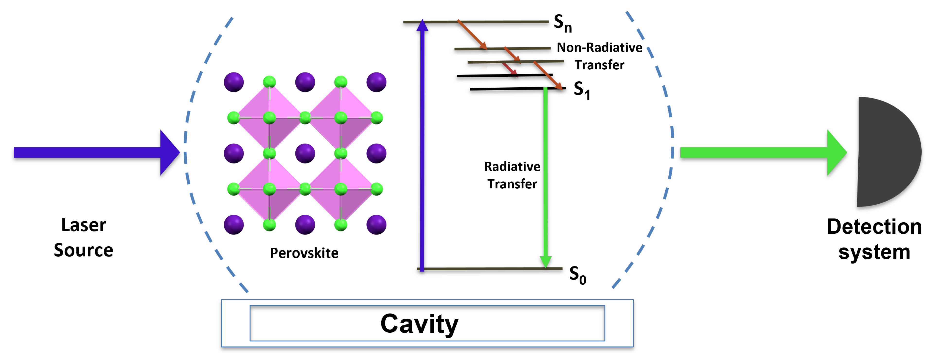
The principle of the filigran used for authenticating banknotes is common knowledge. In summary, when we submit the banknote to a specific optical excitation (illumination at normal incidence), a specific response is induced at the level of the filigran (the image of the filigran becomes visible if we observe it in transparency along the axis joining it to the source). It is not easy to counterfeit such filigrans, which differ from usual 2D images by the fact that they are not visible under grazing illumination. Ultimately, it is this specific response of the filigran that explains why it is a useful tool for authentication. Our goal, roughly expressed, is to conceive quantum filigrans based on the specific optical response of well-chosen fluorophores, in the quantum strong-coupling regime. The scheme of principle of our idea is depicted in Figure 1: a solution containing fluorophores is placed inside a tunable Fabry–Pérot cavity; a fluorophore is resonantly excited by a laser source and absorbs a photon at a wavelength of 440 nm. A part of the energy is lost in an initial non-radiative process, followed by a radiative quantum jump at wavelengths of 530 ± 25 nm.

Figure 1.
Scheme of Quantum Filigran experiment. The blue arrow represents the light emitted by the laser, resonant with the peak of absorption of the fluorophore (440 nm). The green arrow represents the emitted photon. Note that in the strong coupling regime, photons are emitted at two possible wavelengths (530 ± 25 nm), a manifestation of frequency splitting.
This frequency splitting is the signature of quantum strong coupling which is ensured by placing the fluorophore in a cavity resonant at 530 nm (for more details, see Section 4). The single photons emitted one at a time by the fluorophores are filtered in frequency around one of the two emission peaks and collected in a typical fluorescence device consisting of a single photon detector coupled to an acquisition table. The statistical distribution of the arrival times of the photons emitted by the fluorophore is well-approximated by a double exponential distribution. As a last resort, this distribution is, as explained in Section 4), the signature of the presence, at the level of the fluorophore, of two competing non-radiative processes, a short one and a long one. This specific response of the fluorophore (single photon emission, plus frequency splitting and frequency shift, plus specific temporal statistics) is extremely difficult to clone by classical methods; it will play the role of a quantum filigran in our proposal.
3. Fluorophore Coupled to a Resonant Cavity in the Strong-Coupling Regime
3.1. Strong-Coupling with a Perfect Lossless Cavity
Strong-coupling naturally appears if we consider a two-level system (atom, fluorophore) resonantly coupled to an ideal, lossless and isolated, cavity mode. The Hamiltonian describing such a system is well-known. It is the so-called Jaynes–Cumming (J–C) Hamiltonian. It is obtained after performing various approximations (such as dipolar coupling and rotating wave approximation). In an empty cavity, for an atom dipole moment and a perfect polarization and position matching with the mode, the dipolar interaction is equal to the product between the dipole moment and the effective cavity electric field (in the absence of photon). The electric field of the empty cavity is , where is the cavity volume and is the cavity mode frequency. The coupling strength is characterized by .
The J–C Hamiltonian [12] then reads
The parameters of this Hamiltonian are the atomic transition frequency , the cavity mode frequency , and the coupling constant g. When a single dipole (atom/fluorophore) is considered, the state of the system is
where the state stands for dipole in the excited state and no photon in the cavity and stands for dipole in the ground state and one photon in the cavity. The J–C Hamiltonian then reduces to a matrix
It is worth noting that is Hermitian. In what follows, we shall consider a nearly resonant cavity ( so that the detuning = is small).
The new eigenenergies of the coupled system are [13]
where we defined the so-called vacuum Rabi frequency:
At resonance (), the energy difference between the two modes is minimal and equal to . The energy eigenstates are given by
The parameter defines the entanglement strength [3] between the dipole and the cavity mode (). At resonance, entanglement is maximal () and the dressed states have matter and field components of equal weight. The separation between two distinct matter–radiation subsystems is then impossible. Far from resonance ( and ), these states exhibit dominant matter or electromagnetic components. These polaritonic states inherit dispersion relations from their electromagnetic component. Let us note that the pair of eigenenergies and eigenstates are only the lowest of an infinite ladder of pairs. Similar pairs exist for the quantum superposition of states and involving the presence of or photons in the cavity, respectively. Their energy gap at resonance is given by .
In practice, perfectly lossless cavities do not exist and the criterium to enter the strong-coupling regime is that the Rabi frequency must be significantly larger than the widths and related to the cavity mode and matter excitation lifetimes, respectively. In other words, coupling must dominate over dissipative processes. This condition is required to preserve quantum coherence, as the Rabi frequency describes the rate of coherent energy conversions between matter and the radiation field in the dressed states. In general, to increase the coupling g, one needs to select quantum emitters with a strong transition dipole and to confine the electromagnetic field in a small volume. To decrease , high-finesse cavities are required. The team of S. Haroche (Nobel prize 2012), which is at the same time a pioneering and a leading team in the domain of strong coupling, developed high-finesse superconducting cavities cooled down to a few millikelvins, and reached huge values for the coupling factors g by using, as two-level systems, Rydberg atoms resonant with the cavity [14]. In our approach, it is rather the Purcell effect [15] that plays a prior role in increasing the value of g. This explains why we realize strong coupling even at room temperatures, as explained in Section 4.
3.2. Strong-Coupling with a Lossy Cavity
In order to phenomenologically describe losses [16] let us now consider the pure state (3) dynamics described by a non-Hermitian “effective” Hamiltonian where is introduced phenomenologically and, in the basis , reads:
where the parameter is called the cavity decay rate.
The coefficients and are obtained by solving the Schrödinger equation with the non-Hermitian Hamiltonian :
In order to solve the dynamics of such a system, let us diagonalize the above matrix. Upon diagonalization, one finds the following eigenvalues:
where we defined the quantity:
(where represents the detuning). We are first of all interested in the probability of finding the atom in the excited state, the survival probability defined as , so we want to find the expression of . Its general expression reads:
where the constants and are determined by the initial conditions and (coming from the fact that in Equation (9)):
It is worth noting that for one excitation (photon), the phenomenological approach is equivalent to a rigorous dissipative approach using a master equation (see, e.g., Ref. [17] Chapter 6, especially Section 6.2, entitled “Spontaneous emission: From irreversible decay to Rabi oscillations”).
3.3. Weak and Strong-Coupling Regime in the Resonant Case
One can clearly see that two different regimes in the time-domain are possible depending on the values of g and :
- (i)
- (ii)
- For a large coupling constant, , is real, and the eigen-frequencies (Equation (14)) show a different real part, leading to oscillations of the amplitude in the time-domain, known as the strong-coupling regime.
The general solution will not be considered in detail here but we shall focus on the (very) strong-coupling regime, i.e., when . A very good approximation of the solution may be derived in this case by means of power series expansion:
Then, becomes
which gives a survival probability
One can see in this equation that oscillates at the frequency . These oscillations, also called “vacuum Rabi oscillations”, are characteristic of the strong-coupling [17].
3.4. Emission Spectrum in the Strong-Coupling Regime
There exists an alternative way to describe the coupling of a dipole to a lossy cavity, which is conceptually quite different from the ones presented in the previous sections. This model ([18], Chapter 1, Complement 1A) treats the spontaneous emission of an atom coupled to a bounded continuum of electromagnetic modes, with a bandwidth . As previously, the atom is modeled as a two-level system with transition frequency , and the continuum is assumed to have a “Lorentzian” density of states (modes) centered on a frequency and with a bandwidth expressed through the Full Width Half Maximum (FWHM) and from now on taken to be equal to . In particular, while conceptually very different, this model predicts the same temporal behavior as the previous ones. Its interest is that it predicts the distribution in energy of the emitted photons in the continuum which is an observable that one can measure in practice: the so-called vacuum Rabi splitting.
This model is developed in appendix (Supplementary Material), where we show that, in the highly strong-coupling regime, the probability of emitting a photon in mode , denoted obeys
where the cross-term C.T. is given by:
As seen from Equation (21), in the strong-coupling regime , the distribution of emitted photons features two peaks separated by , and of FWHM . Therefore, an “order of magnitude” condition to be able to distinguish the two peaks is:
3.5. Studying Poincaré Recurrences with a Discrete Model of Evolution
As we show now, the weak- to strong-coupling transition can also be interpreted in terms of Poincaré recurrences, in the framework of a discrete model which can be tackled numerically. We have already considered this model in the past, in Refs. [3,19] where we focused on energy conservation, and also showed its good agreement with the Wigner-Weiskopff model [20]. In this model, one considers a single atom coupled to N states j with a “door” distribution centered on the atomic frequency and of variable bandwidth . They represent the distribution of the e-m modes in the cavity. One can then express the evolution equation in a matrix form:
Moreover, one assumes equal and real coupling constants: for all modes j.
The square matrix M can be numerically diagonalised. The program gives back the eigenvalues and eigenvectors of M, which can be used to solve and , using the general expression of their solution
where the are given by the initial conditions:
In order to better understand the implications of our toy model, we plotted the survival probability of the initially excited atom/fluorophore in function of the coupling to the cavity, varying the parameters of the model. These parameters are: which is the density of states in the comb (with equal to the difference for ); N is the number of modes and the coupling between the “atom” and the “cavity”. is thus equal to the “continuum” bandwidth , while the theoretical value of the gamma factor obtained by applying the Fermi golden rule is denoted . It is equal to .
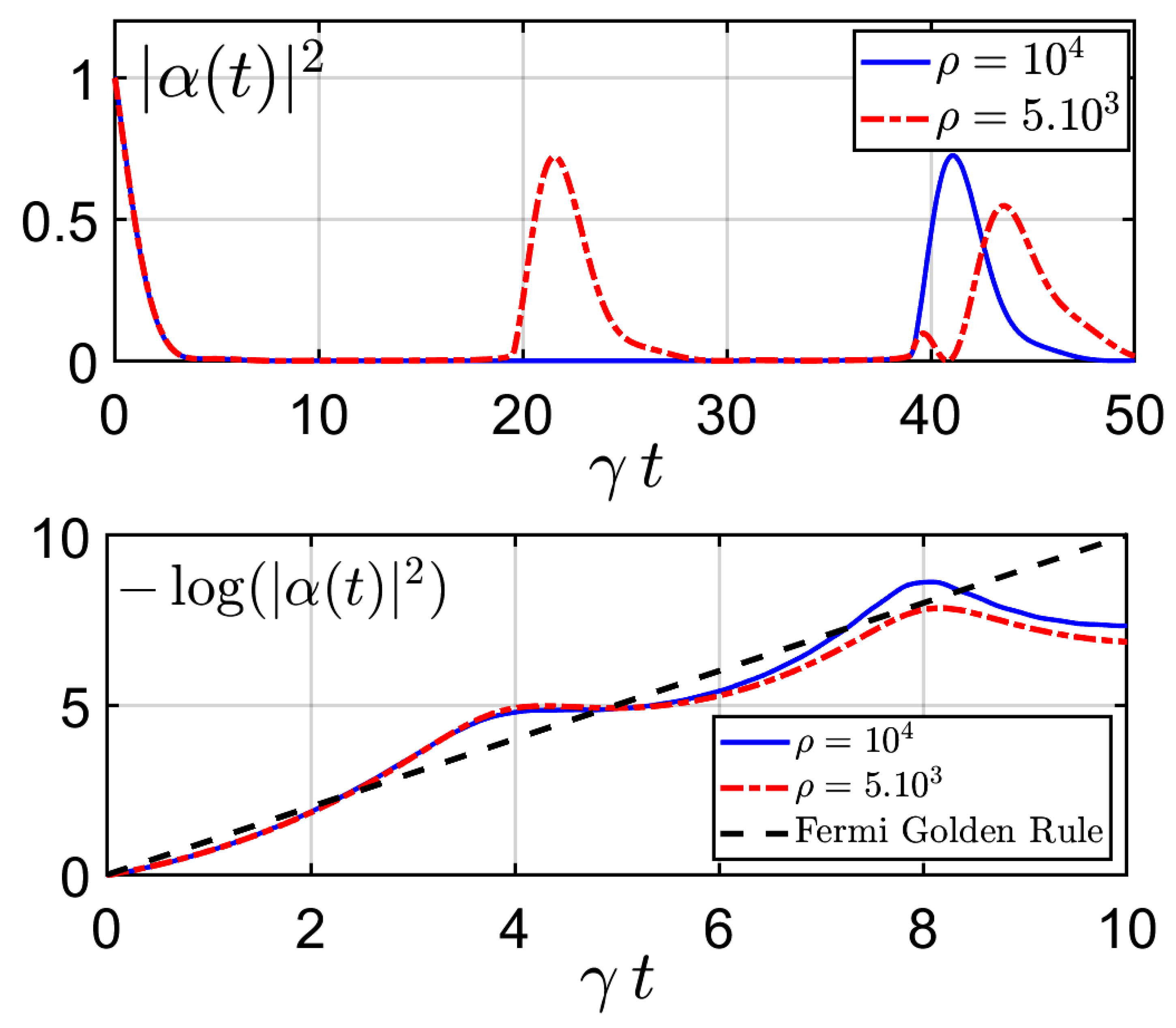
In Figure 2, we plot the survival probability obtained with this numerical method in the weak coupling regime, for two values of the density of modes, adjusting, however, the coupling constant in order to keep constant the theoretical value of the gamma factor obtained by applying the Fermi golden rule. Exponential decay is well observed, in agreement with the Fermi golden rule, but for very long times there appear large “revival” peaks which are an artefact peculiar to the discretization [3]. It is a manifestation of partial Poincaré recurrence due to the fact that when the Hilbert space of the quantum system is of finite dimension, the Poincaré recurrence time is finite (and its value is the smallest common multiple of all the eigenfrequencies of the Hamiltonian in Equation (24)). The Poincaré recurrence time increases when the density of modes increases as we can check comparing the red and blue recurrences, illustrating that, at least in the weak-coupling regime, the Poincaré recurrence goes to infinity in the continuum’s limit.
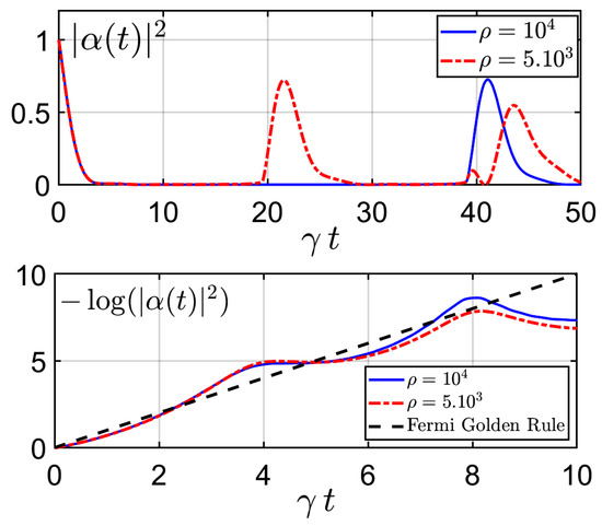
Figure 2.
Survival probability in function of time in the weak coupling regime: linear–linear plot (above) and log–linear plot (below) for two values of the mode density , respecting the scaling constraint constant (where is the decay factor obtained from the Fermi golden rule and the rescaled time).
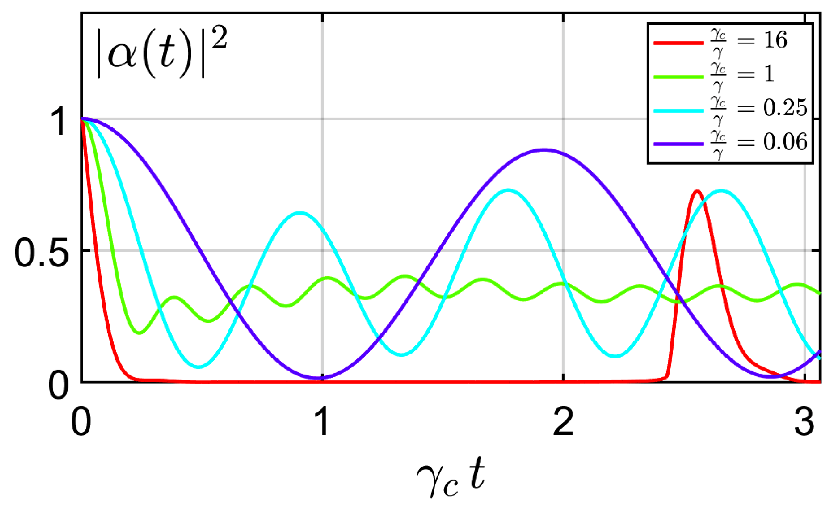
As can be seen in Figure 3, when we vary the bandwidth, keeping constant the spacing between the states in the comb, as well as the gamma factor obtained by applying the Fermi golden rule, the Poincaré recurrence time is constant. This effect is easy to explain in the weak-coupling regime because “active” resonant modes are then confined in an interval of width around the resonant frequency in agreement with time-energy uncertainties; therefore, in the broad spectrum regime (), the physics of the system is unchanged when we vary the bandwidth.
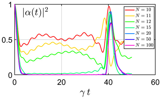
Figure 3.
Survival probability in function of time respecting the scaling constraint constant but varying the number of modes N.
This is no longer true however if we keep the number of modes constant, even when we vary the bandwidth (respecting the scaling constraint constant), as already seen in Figure 2.
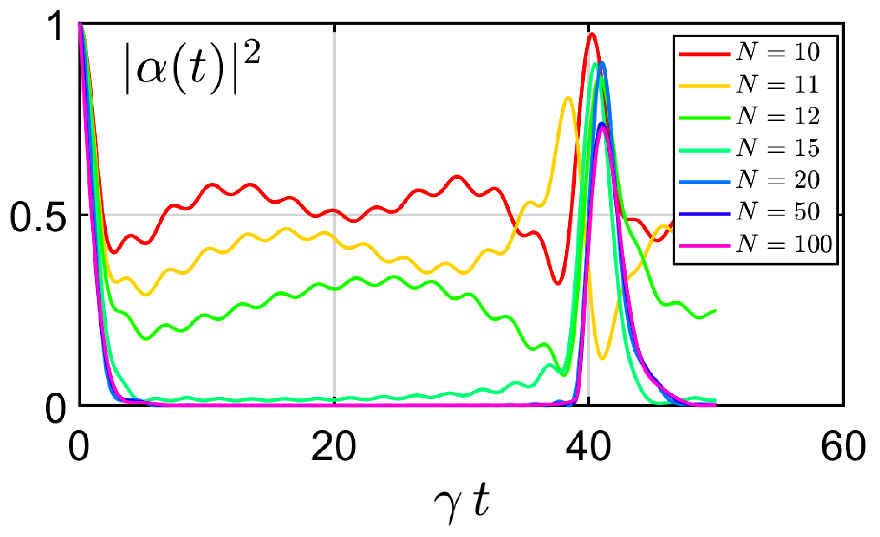
When the number of modes is small enough, new fractional Poincaré recurrences appear, announcing the Rabi oscillations of Figure 4, typical of the strong coupling regime.
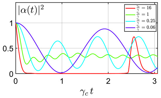
Figure 4.
Survival probability in function of time for various values of . In the weak-coupling regime, the Poincaré recurrence is an artefact of discretization, whereas in the strong-coupling regime Poincaré recurrences become indistinguishable from Rabi oscillations, typical of a system consisting of two coupled modes.
As can be seen from Figure 4, fractional Poincaré recurrences appear at the weak–strong transition (). In the strong-coupling regimes the revivals become indistinguishable from Rabi oscillations. The nature of Poincaré recurrences is clearly different in the weak- and strong-coupling regimes: in the weak-coupling regime they are an artefact of the discretization; in the strong-coupling regime, (fractional) Poincaré recurrences correspond to Rabi oscillations.
4. Experimental Study
4.1. Experimental Protocol
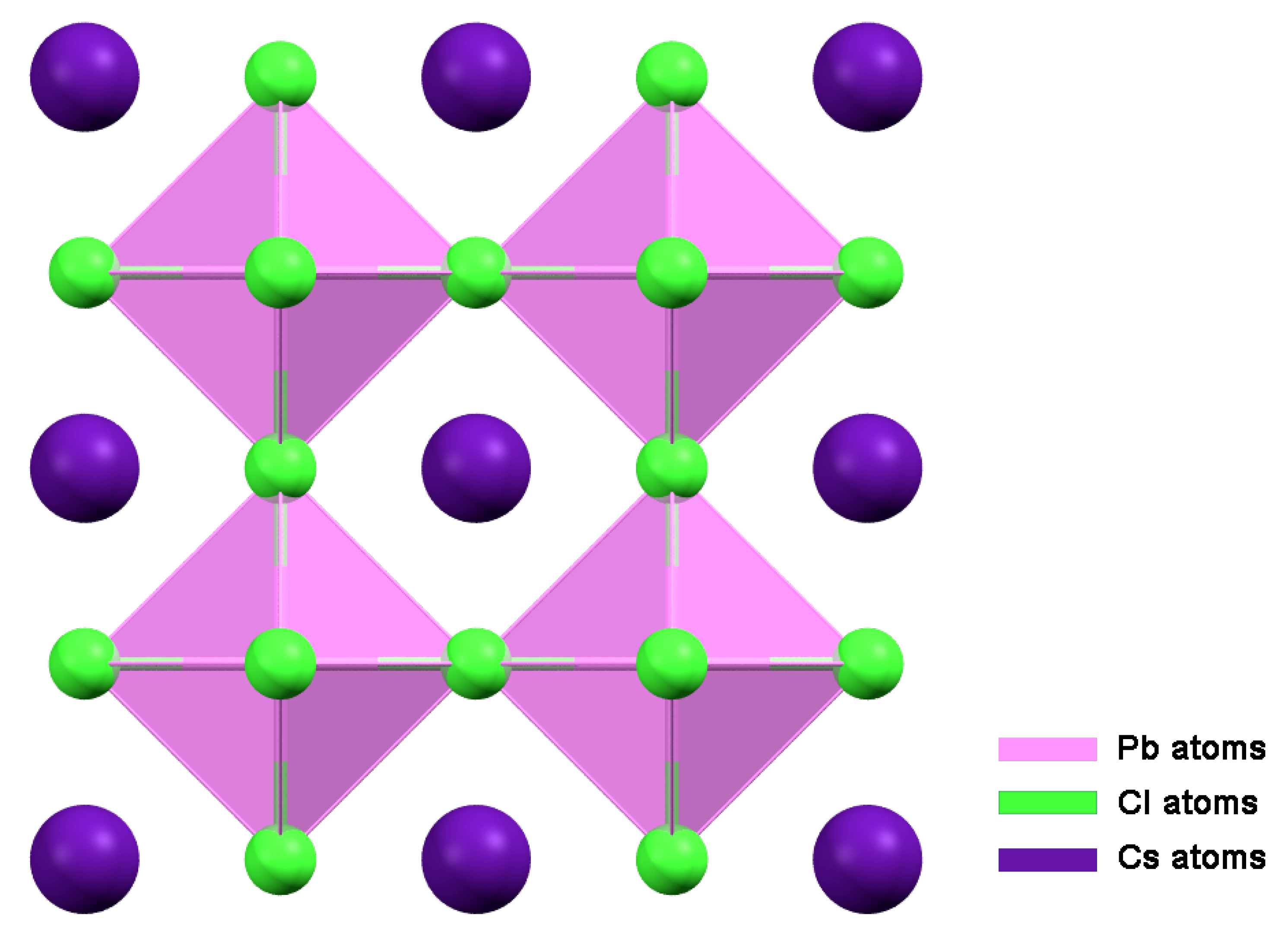
In order to perform the strong-coupling between nanoprobe and the cavity, we fabricated the plasmonic cavity by combining thermal-sputtering (for metal/Al deposition), and spin coating (for controlling the thickness of the cavity and for embedding nanoprobes into the cavity). The obtained cavity has a quality factor of around 70. Later we dissolved perovskite fluorophores (commercially available), at the concentration of 0.1 nM. The schematic structure of perovskite is presented in Figure 5.
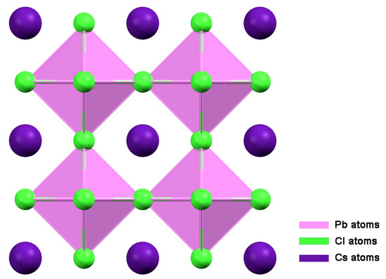
Figure 5.
Structure of CsPbCl perovskite is based on crystal structure from ICSD database 201250 [21].
Subsequently, 10 microliters of the perovskite solution (dissolved in toluen) were transferred into polymer solution (polystyrene(PS), volume 2 mL) used for spin coating in order to place the nanoprobe inside a cavity. The thickness of the cavity was adjusted to achieve resonance ( close to zero, where represents the Bohr frequency of the fluorophores in free space).
The details concerning cavity design, sample preparation, and quality factor estimation are described in Supplementary Materials.
4.2. Results
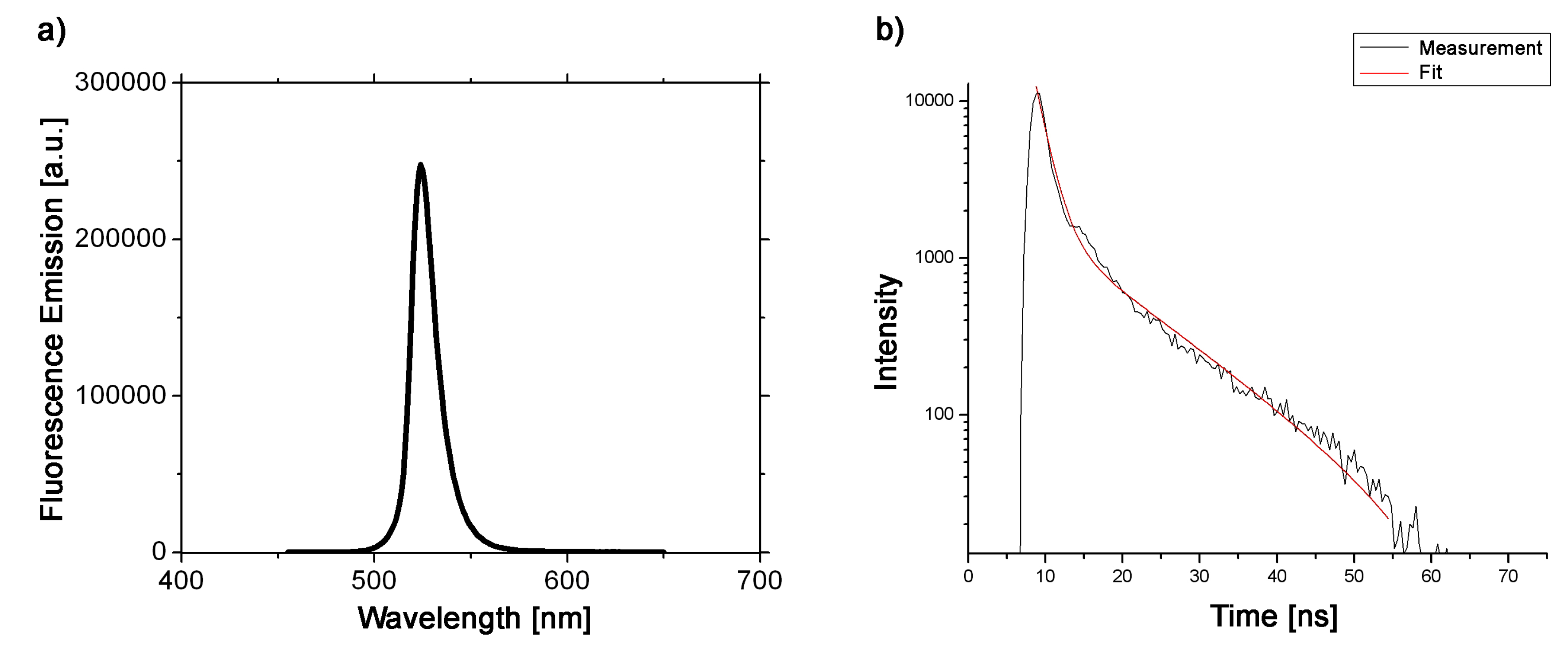
First, we investigate the fluorescence response of the perovskite outside the cavity. Figure 6 shows the fluorescence response of the perovskite probes in solution. The excitation wavelength used for fluorescence measurement was 440 nm. The observed emission spectrum is relatively narrow (for organic and metalorganic compounds), with the maximum around 530 nm and full width half maximum (FWHM) approximately 25 nm.
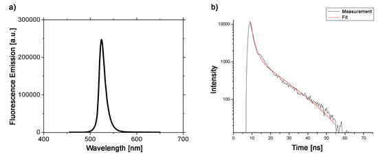
Figure 6.
(a) Fluorescence steady state spectrum of perovskite in solution; (b) Fluorescence decay time response of the perovskite in solution fitted with a double exponential function.
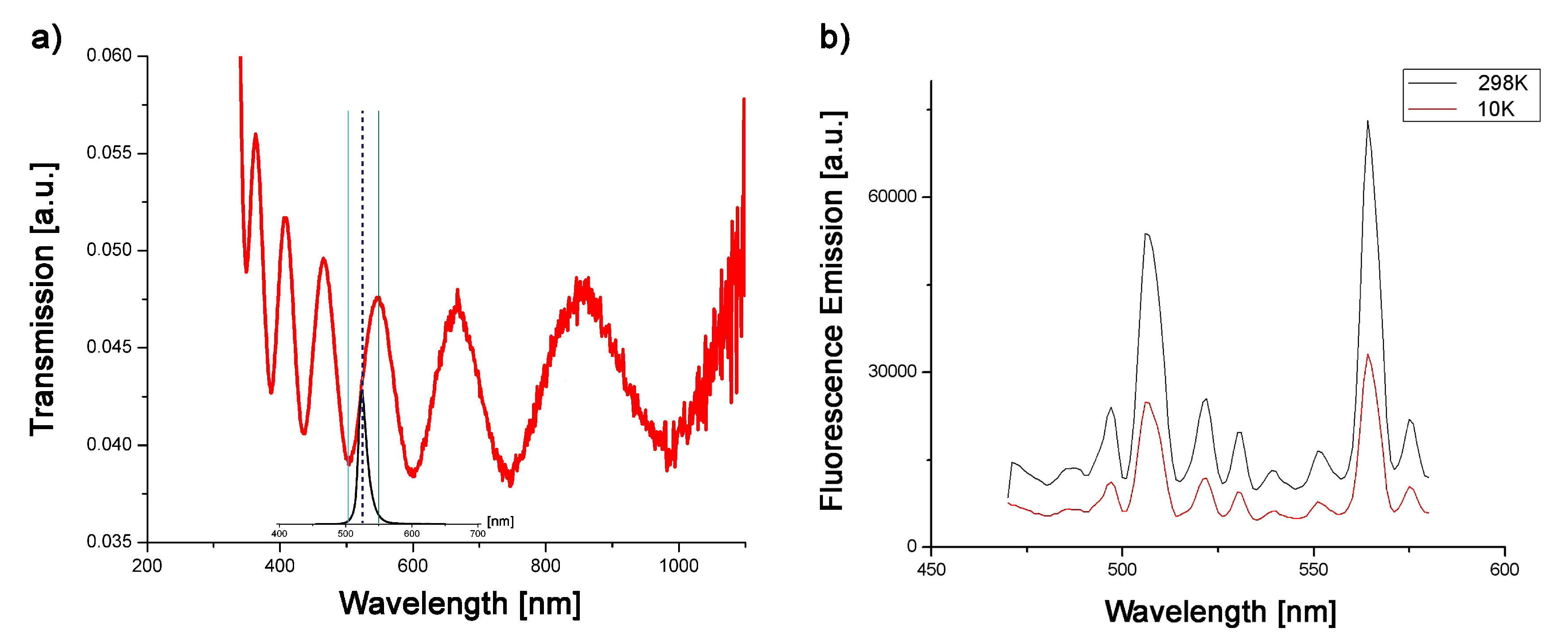
In order to understand better the radiative response, we performed time-resolved measurements of the emitted fluorescence intensity (Figure 6b). The best fits of experimental results are obtained with a double exponential function that gave rise to a long decay time (of ca. 12.2 ns) that is related to the actual lifetime of the probe in this particular environment, and a short decay time (of ca. 1.6 ns), is associated with different nonradiative processes that affect the radiative dynamics of the dye. After that, we perform the steady-state investigation of the perovskite embedded into the plasmonic cavity at two different temperatures (room temperature 298 K and 10K). The sample was excited from outside the cavity; the excess energy is necessary for creating a complex metastable excited state that will firstly follow a complicated non-radiative decay process before arriving at the radiative excited dipole state considered in Section 3. The steady-state response of the perovskite within the cavity is presented in Figure 7 and shows the signature of Rabi splitting that confirms that strong coupling between cavity and probe is achieved. As can be seen from Figure 7b, the splitting remains observable at room temperature, even though the height of the peaks diminished by then due to various sources of decoherence that increase with increasing temperature of the sample. Figure 7a exhibits the typical response of a Fabry–Pérot cavity.

Figure 7.
(a) Optical response of the cavity with emission spectrum from perovskite fluorophores in solution (inset); (b) emission spectrum from perovskite fluorophores in cavity—signature of Rabi splitting.
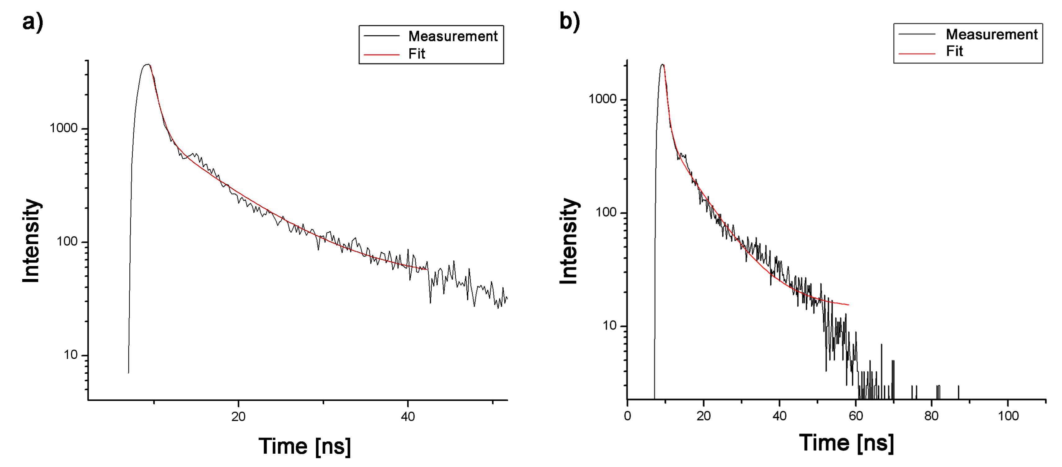
After a steady-state fluorescence study that shows the signature of the strong-coupling through Rabi splitting, the fluorescence time-resolved study reveals the effect of the strong coupling on the dynamics of the excited state. The theoretical decay time of the cavity is comparable, in the strong-coupling regime, to the survival time of the excited state . It can be estimated by measuring the width of one of the Lorentzian peaks of Figure 7. By so doing, we estimate the lifetime of the cavity to be in the picosecond range. The distance between the two peaks makes it possible to estimate the value of the coupling constant g from which the ratio g/ is thus predicted to be equal to 5.9, which confirms once more that we are well in the strong-coupling regime. Results of the measurement show that, as in the case of the probe in solution, the perovskite radiation dynamics within the cavity are best fitted with the double exponential functions. Like the energy splitting, the two decay signatures survive at room temperature (as can be seen from Figure 8. At room temperature (298 K), the perovskite within the cavity gave rise to a long decay time (of ca. 7.7 ns) that is related to the actual lifetime of the probe within the cavity and a short decay time (of ca. 0.87 ns) that is associated with different nonradiative processes that affect the radiative dynamics of the dye. The probe’s lifetime within the cavity is significantly shorter (37%) compared to the lifetime in solution (decay rate increases). Decreasing temperature causes the increase of the lifetime of the probe to the value of 8.1 ns (5%), while the short decay stays unchanged, indicating that non-radiative processes within the cavity are not so strongly affected by the decrease in temperature.
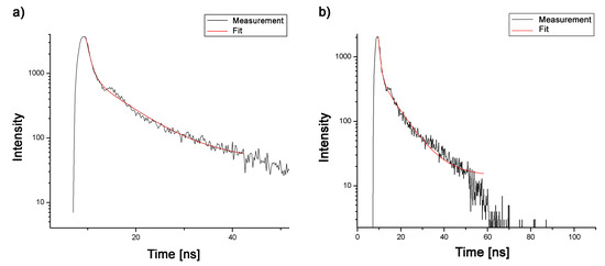
Figure 8.
Fluorescence time-resolved measurements of the perovoskite within plasmonic cavity at two temperatures: (a) 298 K, and (b) 10 K.
The duration of the radiative process, estimated by measuring the width of the Lorentzian emission curve, is quite smaller than the duration of the non-radiative part of the decay process. Among other consequences, the probability that two photons will be emitted at the same time goes to zero, and we are thus always operating in the single photon regime. Due to the coexistence of the (long) fluorescence timescale and of the (short) timescale of the photon emission process, it is impossible for us to put into evidence specific signatures of the strong-coupling such as Rabi oscillations, without speaking about the entanglement between the dipole and the field inside the cavity. However, frequency splitting is directly observable with our device. It constitutes an authentic signature of the quantum strong-coupling, which offers promising perspectives regarding tracing and marking as we shall explain now.
5. Tracing and Marking in the Strong-Coupling Regime
Fluorophores are widely used for tracing and marking [2,22,23,24], but it is uncommon to let them operate in the strong-coupling regime. Recently, strong-coupling has been exploited for potential quantum chip applications using fluorophores attached to oligonucleotide strands and embedded into the cavity [25]. These DNA or RNA oligonucleotide strands offer the possibility of putting the probe in a particular position within the cavity, and/or to link it with a plasmonic nanoobject (for instance a golden nanosphere) playing the same role as an external cavity [26,27,28], but this advantage comes with the relatively high cost of design and purification of oligonucleotides associated with the aging problem (stability of oligonucleotide probes within the cavity). In our approach, combining cavity design, spin coating, and specifically chosen fluorophores, we reach the strong-coupling regime without resorting to DNA strands. Another advantage of this regime is that it increases the signal-to-noise ratio, due to the fact that the frequency of the emitted photons differs from the resonance frequency of the cavity, and from the excitation frequency of the laser as well, which makes it easy to filter out the noise at those frequencies, by using well-chosen frequency filters (as we described in the previous section). The use of a resonant cavity also grandly amplifies the signal, which is a well-known manifestation of the Purcell effect [15]. In summary, our approach reduces noise and increases the signal, directly benefiting the signal-to-noise ratio.
6. Conclusions
In order to prevent counterfeiting, and to be able to authenticate their own manufactured goods, certain brands hide specific DNA branes in their products (clothes for instance), since they are difficult to imitate and can be revealed through DNA sequencing. We propose to use fluorophores in the strong-coupling regime described in the previous sections to realize the same goal. The present manuscript describes the quantum foundation of the strong-coupling and the experimental study of radiation dynamics in the strong-coupling regime. It also highlights how these dynamics can be harnessed in tracing and authentication, due to their unique response and simple detection requirements. The specific signature of strong-coupling is difficult to counterfeit (it also requires good overlap between the cavity resonance and absorption/emission spectrum of the probe), and it is easy to reveal because it needs a basic fluorescence device, is widely commercialized, and is versatile and fast to operate compared to DNA sequencing, for instance. It should be emphasized that instead of using expensive lithography techniques or time-consuming self-assembly processes, the new PUF that we propose here is solely based on the light–matter interaction. It constitutes a compromise between quantum encryption, à la Wiesner [11], and classical encryption. This approach opens a large field of potential applications.
Supplementary Materials
The following supporting information can be downloaded at: https://www.mdpi.com/article/10.3390/app12189238/s1, Figure S1: Two-level system in a cavity.
Author Contributions
Conceptualization: T.D.; Theoretical study: T.D., M.H. and E.L. Experimental study: D.M., B.B. and B.K.; Writing—original draft: T.D. and B.K.; Discussion: all authors; Writing—review & editing: all authors. All authors have read and agreed to the published version of the manuscript.
Funding
Biological and bioinspired structures for multispectral surveillance, funded by NATO SPS (NATO Science for Peace and Security), the Office of Naval Research Global through the Research Grant N62902-22-1-2024, the John Templeton foundation (grant 60230, Non-Linearity and Quantum Mechanics: Limits of the No-Signaling Condition, 2016–2019).
Institutional Review Board Statement
Not applicable.
Informed Consent Statement
The authors declare no conflict of interest. The funders had no role in the design of the study; in the collection, analyses, or interpretation of data; in the writing of the manuscript, or in the decision to publish the results.
Data Availability Statement
Not applicable.
Acknowledgments
All authors acknowledge the support of Sylvain Desprez-Materia Nova regarding metal deposition. B.K. acknowledge support of the project Biological and bioinspired structures for multispectral surveillance, funded by NATO SPS (NATO Science for Peace and Security) 2019–2022. B.B. and B.K. acknowledge funding provided by the Institute of Physics Belgrade, through the institutional funding by the Ministry of Education, Science, and Technological Development of the Republic of Serbia. D.M., B.B. and B.K. acknowledge the support of the Office of Naval Research Global through the Research Grant N62902-22-1-2024. Additionally, B.K. acknowledges support from F.R.S.-FNRS Belgium. E.L. acknowledges support from Ecole Doctorale 352, Aix-Marseille. M.H. acknowledges support from the John Templeton foundation (grant 60230, Non-Linearity and Quantum Mechanics: Limits of the No-Signaling Condition, 2016–2019).
Conflicts of Interest
The authors declare no conflict of interest.
References
- Sengupta, P.; Khanra, K.; Chowdhury, A.R.; Datta, P. Lab-on-a-chip sensing devices for biomedical applications. In Bioelectronics and Medical Devices from Materials to Devices—Fabrication, Applications and Reliability, 1st ed.; Pal, K., Kraatz, H.-B., Khasnobish, A., Bag, S., Banerjee, I., Kuruganti, U., Eds.; Woodhead Publishing: Sawston, UK, 2019; pp. 47–95. [Google Scholar]
- Lakowicz, J.R. Principles of Fluorescence Spectroscopy, 3rd ed.; Springer: New York, NY, USA, 2006; pp. 623–740. [Google Scholar]
- Kolaric, B.; Maes, B.; Clays, K.; Durt, T.; Caudano, Y. Strong Light-Matter Coupling as a New Tool for Molecular and Material Engineering: Quantum Approach. Adv. Quantum Technol. 2018, 1, 1800001. [Google Scholar] [CrossRef]
- Shalabney, A.; George, J.; Hiura, H.; Hutchison, J.A.; Genet, C.; Hellwig, P.; Ebbesen, T.W. Enhanced Raman Scattering from Vibro-Polariton Hybrid States. Angew. Chem. Int. Ed. 2015, 54, 7971–7975. [Google Scholar] [CrossRef]
- Orgiu, E.; George, J.; Hutchison, J.A.; Devaux, E.; Dayen, J.F.; Doudin, B.; Stellacci, F.; Genet, C.; Schachenmayer, J.; Genes, C.; et al. Conductivity in organic semiconductors hybridized with the vacuum field. Nat. Mater. 2015, 14, 1123–1129. [Google Scholar] [CrossRef] [PubMed]
- Vergauwe, R.M.A.; George, J.; Chervy, T.; Hutchison, J.A.; Shalabney, A.; Torbeev, V.Y.; Ebbesen, T.W. Quantum Strong Coupling with Protein Vibrational Modes. J. Phys. Chem. Lett. 2016, 7, 4159. [Google Scholar] [CrossRef]
- Ramezani, M.; Berghuis, M.; Gómez Rivas, J. Strong light–matter coupling and exciton-polariton condensation in lattices of plasmonic nanoparticles (Review). J. Opt. Soc. Am. B Opt. Phys. 2019, 36, E88–E103. [Google Scholar] [CrossRef]
- Pelton, M.; Storm, S.D.; Leng, H. Strong coupling of emitters to single plasmonic nanoparticles: Exciton-induced transparency and Rabi splitting. Nanoscale 2019, 11, 14540–14552. [Google Scholar] [CrossRef]
- Pappu, R.; Recht, B.; Taylor, R.; Gershenfeld, N. Physical One-Way Functions. Science 2002, 297, 2026–2030. [Google Scholar] [CrossRef] [PubMed]
- Pavlović, D.; Rabasović, M.D.; Krmpot, A.J.; Lazović, V.; Ćurčić, S.; Stojanović, D.V.; Jelenković, B.; Zhang, W.; Zhang, D.; Vukmirović, N.; et al. Naturally safe: Cellular noise for document security. J. Biophotonics 2019, 12, e201900218. [Google Scholar] [CrossRef]
- Wiesner Quantum Money. Available online: https://wiki.veriqloud.fr/index.php?title=WiesnerQuantumMoney (accessed on 1 September 2022).
- Jaynes, E.T.; Cummings, F.W. Comparison of Quantum and Semiclassical Radiation Theories with Application to the Beam Maser. Proc. IEEE 1963, 51, 89–109. [Google Scholar] [CrossRef]
- Bina, M. The coherent interaction between matter and radiation. Eur. Phys. J. Spec. Top. 2012, 203, 163–183. [Google Scholar] [CrossRef]
- Haroche, S.; Raimond, J.M. Exploring the Quantum—Atoms, Cavities and Photons; Oxford University Press: Oxford, UK, 2007. [Google Scholar]
- Carminati, R.; Greffet, J.J.; Henkel, C.; Vigoureux, J. Radiative and non-radiative decay of a single molecule close to a metallic nanoparticle. Opt. Commun. 2006, 261, 368–375. [Google Scholar] [CrossRef]
- Lassalle, E. Environment Induced Modifications of Spontaneous Quantum Emissions. Ph.D. Thesis, University of Marseille, Marseille, France, 2019. [Google Scholar]
- Dutra, S.M. Cavity Quantum Electrodynamics: The Strange Theory of Light in a Box, 1st ed.; John Wiley & Sons: Hoboken, NJ, USA, 2005. [Google Scholar]
- Grynberg, G.; Aspect, A.; Fabre, C. Introduction to Quantum Optics: From the Semi-Classical Approach to Quantized Light, 1st ed.; Cambridge University Press: Cambridge, UK, 2010. [Google Scholar]
- Debierre, V.; Goessens, I.; Brainis, E.; Durt, T. Fermi’s golden rule beyond the zeno regime. Phys. Rev. A 2015, 92, 023825. [Google Scholar] [CrossRef]
- Weisskopf, V.; Wigner, E. Berechnung der natürlichen linienbreite auf grund der diracschen lichttheorie. Z. Für Phys. 1930, 63, 54–73. [Google Scholar] [CrossRef]
- Hunton, J.; Nelmes, R.J.; Moyer, G.M.; Eriksson, V.R. High resolution study of cubic perovskites by elastic neutron diffraction: CsPbCl3. J. Phys. C Solid State Phys. 1979, 12, 5393. [Google Scholar]
- Cowen, E.A.; Ward, K.B. Chemical Plume Tracing. Environ. Fluid Mech. 2002, 2, 1–7. [Google Scholar] [CrossRef]
- Anti-Counterfeiting Technology Guide; European Union Intellectual Property Office: Alicante, Spain, 2021.
- Trace Chemical Sensing of Explosives, 1st ed.; Woodfin, R.L. (Ed.) Wiley: Hoboken, NJ, USA, 2006. [Google Scholar]
- Chan, W.P.; Chen, J.H.; Chou, W.L.; Chen, W.Y.; Liu, H.Y.; Hu, H.C.; Jeng, C.C.; Li, J.R.; Chen, C.; Chen, S.Y. Efficient DNA-Driven Nanocavities for Approaching Quasi-Deterministic Strong Coupling to a Few Fluorophores. ACS Nano 2021, 15, 13085–13093. [Google Scholar] [CrossRef] [PubMed]
- Punj, D.; Regmi, R.; Devilez, A.; Plauchu, R.; Moparthi, S.B.; Stout, B.; Bonod, N.; Rigneault, H.; Wenger, J. Self-Assembled Nanoparticle Dimer Antennas for Plasmonic-Enhanced Single-Molecule Fluorescence Detection at Micromolar Concentrations. ACS Photonics 2015, 2, 1099–1107. [Google Scholar] [CrossRef]
- Busson, M.; Rolly, B.; Stout, B.; Bonod, N.; Bidault, S. Accelerated single photon emission from dye molecule-driven nanoantennas assembled on DNA. Nat. Commun. 2012, 3, 962. [Google Scholar] [CrossRef] [PubMed]
- Busson, M.P.; Rolly, B.; Stout, B.; Bonod, N.; Wenger, J.; Bidault, S. Photonic Engineering of Hybrid Metal—Organic Chromophores. Angew. Chem. Int. Ed. 2012, 51, 11083–11087. [Google Scholar] [CrossRef] [PubMed] [Green Version]
Publisher’s Note: MDPI stays neutral with regard to jurisdictional claims in published maps and institutional affiliations. |
© 2022 by the authors. Licensee MDPI, Basel, Switzerland. This article is an open access article distributed under the terms and conditions of the Creative Commons Attribution (CC BY) license (https://creativecommons.org/licenses/by/4.0/).