A Quasi-Quadratic Inverse Scattering Approach to Detect and Localize Metallic Bars within a Dielectric

Abstract

The inverse scattering problem related to the localization of metal bars embedded within a finite-dimensional dielectric was studied in two-dimensional geometry. The dielectric was placed in air and illuminated from the outside using a linear microwave source and a multi-monostatic configuration. The discontinuity at the interface between the air and the dielectric causes reflections that are neglected if a simple linear Born approximation of scattering is assumed. Herein, a new formulation was proposed based on a quadratic approximation of the scattering equation. The formulation maintained the interaction between the metal bars and the dielectric edge, whereas the mutual coupling between the bars was neglected. By exploiting the knowledge of the permittivity of the dielectric and the shape of its section, a relatively simple approximate expression for the scattered field was derived, which allowed for formulation of an inverse linear problem. Numerical examples demonstrated the feasibility of this approach.

1. Introduction

Microwave inverse scattering is a suitable method for non-destructive testing (NDT) applications. It is based on the ability of the electromagnetic field to penetrate and propagate inside dielectric materials, at frequencies in the microwave band, and on the effects on the propagation of the objects embedded inside the background medium [1]. Ground-penetrating radar (GPR) is one of the most interesting microwave-based techniques, and it is applied in many fields, ranging from geophysics to archeology and civil engineering [2,3,4,5,6].

The study of electromagnetic scattering from cylindrical objects embedded inside a homogeneous dielectric is useful for schematizing many different situations, such as the localization of buried pipelines [7], tree root reconstruction [8], grid diagnostics [9,10], and reinforced concrete monitoring [11,12].

In particular, the diagnosis and monitoring of reinforced concrete structures are of great interest within civil engineering. The bars’ number, diameter, and deployment, together with the concrete cover thickness, are important parameters attesting to the correct structural behavior towards external mechanical stress and long-lasting structures. However, the details of the structural design in terms of such parameters can be lost and must be recovered. Moreover, the structure can be damaged during its life by concrete corrosion or if some bars oxidize, with a diameter smaller than the nominal one. Many destructive and non-destructive methods already exist for acquiring information about materials and structures within civil engineering. Conventional destructive methods usually require samples of the structure under test to be taken, for instance by drilling and coring, or removal of some external layers in order to allow visual inspection of the internal status of the structure. Such methods have the disadvantage of being invasive and providing only punctual information. On the contrary, methods based on NDT techniques do not damage or modify the structure under test and make in situ diagnostics and monitoring possible. The currently available NDT methods for the investigation of reinforced concrete structures are based on a variety of different physical phenomena. Acoustic methods (sonic and ultrasonic frequencies) [13], infrared thermography [14], magnetic flux leakage (MLF) [15], eddy currents [16], optical fibers [17,18], and electromagnetic radar-based methods [5] have been extensively studied. In [15] and the references therein, MLF is discussed, and the experimental results pave the way for its application in concrete bar detection. In [19], a comparison between a destructive method and a non-destructive method based on an ultrasonic pulse for concrete strength measurement is presented, and, in the same paper, GPR measurements are used as a complementary tool to investigate the structure.

Among the NDT methods for reinforced concrete investigation, those based on electromagnetic propagation and scattering, such as radar and GPR, allow contactless measurements to be performed. This feature is very attractive because makes it possible to perform flexible measurements, and it even allows for operation in remote sensing configurations [20]. On the other hand, data processing is challenging for several reasons. Contactless measurements are affected by the strong reflection from the interface between the air and concrete. Additionally, the final result of a commercial GPR is a radargram whose interpretation is not immediate, except in very simple cases, and the need to properly model the electromagnetic scattering phenomenon and formulate an inverse problem arises [21,22].

The focus of this paper is on the mathematical modeling of the scattering phenomenon and on the study of the related inversion algorithm.

Microwave imaging requires the modeling and solving of an inverse electromagnetic scattering problem, which is intrinsically non-linear. The operator relating the external scattered field to the internal dielectric contrast can be expanded in a Taylor operatorial series. In particular, the scattered field depends on the contrast and on the internal field. The internal field, in turn, satisfies a Fredholm equation that can be expanded into the well-known Neumann series and then substituted into the external equation [23,24]. Consideration of only the first term implies linearization, whereas keeping the first two terms of the series brings the quadratic approximation that was considered in the following. In this sense, the quadratic approximation represents the lower degree of non-linearity. From the physical point of view, linearization corresponds to considering each portion of the investigation domain as if it were standing alone in free space, whereas the quadratic approximation can be interpreted as keeping a mutual coupling between different parts of the investigation domain. Similarly, cubic, quartic, and higher order terms would consider “multiple” interactions, which are neglected in the present paper.

There are many different scattering models that allow for the obtaining of algorithms suitable for the reconstruction of desired unknowns [25]. Focusing algorithms, such as backpropagation and backprojection, and approximations, such as the well-known Born, distorted Born, Rytov, and Kirchhoff, fall within the class of linear models of scattering [5]. Linearity allows for dealing with inverse problems in which the attainable resolution can be forecast, and well-assessed techniques against noise are at hand. However, linear models neglect mutual interactions inside the structure and result in the qualitative reconstruction of the region under investigation [26]. On the other hand, preserving the full non-linearity results in algorithms that usually require a huge computational effort, are often solved using non-deterministic procedures, and do not guarantee global convergence to the solution [26]. To avoid such drawbacks, strategies that provide a moderate degree of non-linearity are attractive and worth investigating [27].

In this framework, a quadratic approximation of the scattering phenomenon is demonstrated to be a good compromise between the full non-linear model and the linearized one [28,29]. Additionally, a formulation that includes all the a priori information can be helpful when dealing with partially known structures. This approach has been considered in [9,10] in which a linear approximation was adopted.

Another element that must be considered is measurement configuration. Full-view illumination allows for the collection of more information than a limited aspect one. However, sometimes the structure is not accessible from all around, and only reflection-mode illumination, which is typical, for instance, of ground-penetrating radar applications, is allowed.

The approach proposed here was already briefly presented in the conference paper [30]. In the present extended paper, the analytical details of the proposed model are explicitly derived, and a critical study of the operator is performed. Moreover, several new examples are presented, and the role of the threshold in the detection is shown.

The problem was formulated in canonical two-dimensional geometry: metallic bars embedded into a lossless dielectric homogeneous medium, and in turn, embedded in free space. The electric field polarization was assumed to be parallel to the vertical bars, thus providing a scalar problem. An “almost” quadratic approximation of the problem was derived, which allowed for the achievement of, for the geometry at hand, a synthetic formulation where some of the involved coefficients can be evaluated analytically, thus reducing the computational burden. The data of the problem were the multi-monostatic scattered fields observed at different frequencies. The structure was tested using incident fields radiated by filamentary electric sources placed at different positions along a straight segment outside the investigated region. The bars were electrically conducting cylinders with circular cross-sections whose radii are known. The problem was formulated as the detection and localization of an unknown number of bars inside a pre-determined grid of “candidate” positions. The result of the inversion algorithm is an image showing spots where the bars were detected. To put the proposed approach in the context of reinforced concrete testing, the numerical examples reported in the following were made using realistic values for the dielectric section dimensions and the bar diameter, number, and position.

The paper is organized as follows: in Section 2, the problem is first formulated in operatorial form, and then its expression in the considered geometry is derived; in Section 3, the inverse problem and the related imaging algorithm are presented; and in Section 4, numerical examples are presented. Conclusions follow.

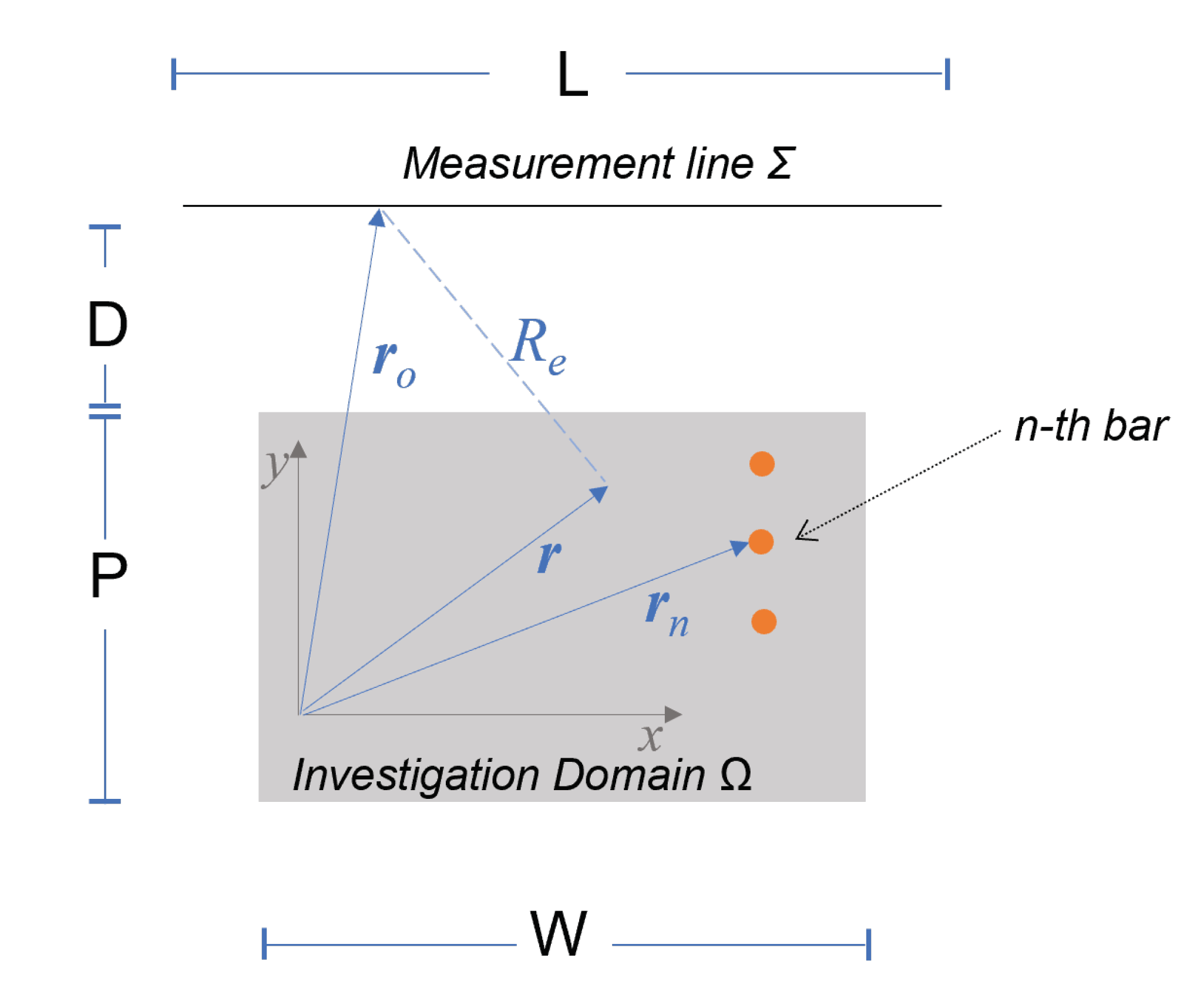
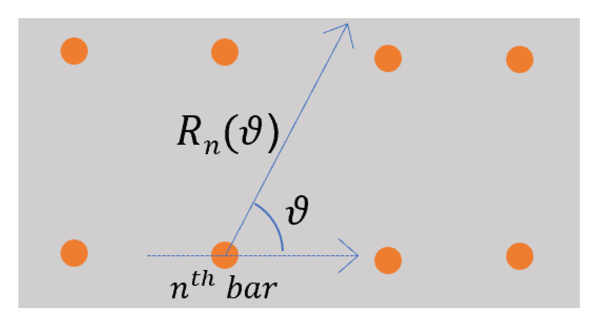
2. Mathematical Formulation

A two-dimensional scalar problem is considered, in which the geometry is invariant along the z-axis of a Cartesian reference system, and the electric field is z-polarized. The investigation domain $\mathsf{\Omega }$ is a limited portion of the $xy$ plane and is filled with a dielectric of the known relative permittivity ${\epsilon }_r$. The external region is free space, whereas, inside $\mathsf{\Omega }$, there are N circular metallic objects, representing the section of circular cylinders whose radii are a. Their positions are indicated by ${\mathbf{r}}_n=(x_n,y_n)$ and $n=1,\dots ,N$. The scene is illuminated by a z-polarized line source placed at different positions along the line $\mathsf{\Sigma }$. A multi-monostatic configuration is assumed in which the scattered field is observed at the same source positions, that is, at $N_o$ observation points over $\mathsf{\Sigma }$. See Figure 1 for the geometry.

Figure 1. Geometry of the problem and reference system. The investigation domain is the rectangle of size $W\times P$ placed at distance D from the measurement line, whose length is L.

The scattering equations are formalized as follows [31]:

$$E_s={\mathbb{A}}_e\left[\chi E\right]$$

(1)

$$E=E_i+{\mathbb{A}}_i\left[\chi E\right]$$

(2)

where $E_i$ and E are the incident and the total field inside $\mathsf{\Omega }$, respectively; $\chi$ is the normalized contrast between the internal and external region; and ${\mathbb{A}}_e$, ${\mathbb{A}}_i$ are linear operators whose kernel is the Green’s function of the scattering problem, calculated outside and inside $\mathsf{\Omega }$, respectively. $E_s$ is the scattered field outside $\mathsf{\Omega }$. It is well known that the inverse problem related to (1) and (2), that is, recovering $\chi$ from the knowledge of $E_s$ and $E_i$, is non-linear. The non-linearity is due to the presence of the total field E in (1), which in turn should be recovered by solving (2).

The usual linear approximation is the Born approximation, in which the total field in (1) is replaced by the incident field [29]. Taking into account a further term in the operator series expansion, that is, replacing the total field on the right-hand side of (2) with the incident field and then substituting the result in (1), the so-called quadratic approximation of the scattered field is achieved [31]:

$$E_s={\mathbb{A}}_e\left[\chi E_i\right]+{\mathbb{A}}_e\left[\chi {\mathbb{A}}_i\left[\chi E_i\right]\right].$$

(3)

2.1. Quasi-Quadratic Approximation of the Scattered Field

To separate the contribution of the bars from that of the dielectric whose permittivity and shape are assumed to be known, the contrast is represented as follows:

$$\chi \left(\mathbf{r}\right)={\chi }_0-jf\left(\mathbf{r}\right),\mathrm{with}\mathbf{r}\in \mathsf{\Omega }$$

(4)

where ${\chi }_0={\epsilon }_r-1$ is constant over $\mathsf{\Omega }$, and

$$f\left(\mathbf{r}\right)=\frac{\sigma \zeta }{k}\sum _{n=1}^N\varphi \left(\right|\mathbf{r}-{\mathbf{r}}_n\left|\right),$$

(5)

where $\sigma$ is the bar’s conductivity, $\zeta$ is the free space impedance, k is the free space wavenumber, and

$$\varphi \left(r\right)=\left\{\begin{array}{c}1r⩽a\hfill \\ 0r>a\hfill \end{array}\right.$$

(6)

Using (4), the quadratic approximation of the scattered field in (3) can be recast as:

$$\begin{array}{c}\hfill E_s={\chi }_0{\mathbb{A}}_e\left[E_i\right]+{\chi }_0^2{\mathbb{A}}_e\left[{\mathbb{A}}_i\left[E_i\right]\right]-j{\mathbb{A}}_e\left[f{E}_i\right]\\ \hfill -j2{\chi }_0{\mathbb{A}}_e\left[{\mathbb{A}}_i\left[f{E}_i\right]\right]-{\mathbb{A}}_e\left[f{\mathbb{A}}_i\left[f{E}_i\right]\right].\end{array}$$

(7)

The quasi quadratic approximation proposed in this paper consists of neglecting the last term in (7). In this way, mutual scattering between the bars is neglected, retaining the interaction between the bars and the surrounding dielectric. Furthermore, the first two terms on the right-hand side of (7) represent the quadratic approximation of the scattered field when no bars are present. Such terms can be calculated, provided that the dielectric shape and permittivity are known, and subtracted from the actual (measured/simulated) scattered field. By denoting such a difference by ${\widehat{E}}_s$, the problem can be formulated as the solution to the following equation:

$$\widehat{E}=-j{\mathbb{A}}_e\left[f{E}_i\right]-j2{\chi }_0{\mathbb{A}}_e\left[{\mathbb{A}}_i\left[f{E}_i\right]\right]$$

(8)

where the relationship between the data, at the first member, and the unknown, i.e., the function $f\left(\mathbf{r}\right)$, is linear.

The explicit computation of (8) is now in order. By exploiting the Green’s function expression in the two-dimensional case, the following results are obtained:

$${\mathbb{A}}_e\left[u\right]=-j\frac{k^2}{4}\underset{\mathsf{\Omega }}{\int \int }{H}_0^{\left(2\right)}\left(k{R}_e\right)u\left(\mathbf{r}\right)d\mathbf{r}$$

(9)

$${\mathbb{A}}_i\left[u\right]=-j\frac{k^2}{4}\underset{\mathsf{\Omega }}{\int \int }{H}_0^{\left(2\right)}\left(k{R}_i\right)u\left(\mathbf{r}\right)d\mathbf{r}$$

(10)

$$E_i=-\frac{k\zeta }{4}{H}_0^{\left(2\right)}\left(k{R}_e\right)$$

(11)

where $R_e=|\mathbf{r}-{\mathbf{r}}_o|$, with ${\mathbf{r}}_o\in \mathsf{\Sigma }$, is the distance between a source/observation and a point inside the investigation domain, $R_i=|\mathbf{r}-{\mathbf{r}}^{\prime }|$, with ${\mathbf{r}}^{\prime }\in \mathsf{\Omega }$, is the distance between two points of the investigation domain; $u\left(\mathbf{r}\right)$ stands for either $E_i$ or $f{E}_i$; $H_0^{\left(2\right)}$ is the Hankel function of zero order and second kind, and the unitary current source is assumed. After some non-trivial passages, as reported in Appendix A, the following results are obtained:

$$\widehat{E}(k,{\mathbf{r}}_o)=\sum _{n=1}^N{C}_n\left(k\right){\left[H_0^{\left(2\right)}\left(k|{\mathbf{r}}_o-{\mathbf{r}}_n|\right)\right]}^2$$

(12)

Equation (12) appears relatively simple, as the Hankel functions act as a sort of pulse centered on the unknown bar positions, and the coefficients $C_n$ do not depend on the observation point. Their expression is:

$$\begin{array}{cc}\hfill C_n\left(k\right)& =\pi \sigma {\zeta }^2{\left(\frac{ka}{4}\right)}^2\left\{1-j2{\chi }_0{\left(\frac{ka}{2}\right)}^2\right.·\hfill \\ \hfill & \left.\left[1-{\left(\frac{ka}{2}\right)}^2-\frac{j}{\pi }(1-2log\left(ka\right))\right]-j\frac{{\chi }_0}{2}{A}_n\right\}\hfill \end{array}$$

(13)

where

$$\begin{array}{cc}\hfill A_n=& \underset{0}{\overset{2\pi }{\int }}\frac{{\left(k{R}_n\right)}^2}{2}\left[J_0\left(k{R}_n\right)H_0^{\left(2\right)}\left(k{R}_n\right)+\right.\hfill \\ \hfill & \left.J_1\left(k{R}_n\right)H_1^{\left(2\right)}\left(k{R}_n\right)\right]d\theta \hfill \end{array}$$

(14)

In (14), the dependence on the integration variable $\theta$ stands in $R_n\left(\theta \right)$, i.e., the distance between the center of the n-th bar and the point on the dielectric/air interface along the $\theta$ direction, as shown in Figure 2.

Figure 2. Reference system used to compute the integral in (14).

It is noteworthy that $A_n$ considers the nth bar position inside the dielectric and the shape of $\mathsf{\Omega }$ itself. Its computation can be performed offline because it does not depend on the observation point’s position.

2.2. Inverse Problem Formulation

Equation (12) allows the formulation of the inverse problem as the detection and localization of bars within a predetermined number $N_b>N$ of “candidate” positions. Following the same approach as in [9], we define a new discrete function $\gamma \left(n\right)$, $n=1,\dots ,N_b$, whose value is 1 if the $n\mathrm{th}$ position is occupied by a bar; otherwise, it is equal to 0. Thus, the problem is recast as a discrete equation as follows:

$$\widehat{E}(k,{\mathbf{r}}_o)=\sum _{n=1}^{N_b}{C}_n\left(k\right){\left[H_0^{\left(2\right)}\left(k|{\mathbf{r}}_o-{\mathbf{r}}_n|\right)\right]}^2\gamma \left(n\right)$$

(15)

where $\gamma \left(n\right)$ plays the role of an unknown.

3. Discretization and Inversion Algorithm

The data are collected at $N_k$ wavenumbers, equally spaced at the interval $[k_{min},k_{max}]$. In the following numerical examples, $\mathsf{\Sigma }$ belongs to the straight line $y=Y_o$, and the data are collected at $N_o$ equally spaced observation points of the abscissa $x_{op},p=1,\dots ,N_o$. Thus, (15) yields the following equation:

$$\left[\begin{array}{c}{E}_{11}\\ \dots \\ E_{1N_k}\\ \dots \\ E_{N_{o}1}\\ \dots \\ E_{N_o{N}_k}\end{array}\right]=\left[\begin{array}{ccc}{G}_{111}& \dots & G_{11N_b}\\ \dots & \dots & \dots \\ G_{N_o{N}_{k}1}& \dots & G_{N_o{N}_k{N}_b}\end{array}\right]\times \left[\begin{array}{c}\gamma \left(1\right)\\ \dots \\ \gamma (N_{b)}\end{array}\right]$$

(16)

where

• $E_{lp}=\widehat{E}(k_l,x_{op})$, $l=1,\dots ,N_k;p=1,\dots ,N_o$ are the data with respect to wavenumber and observation point,
• $G_{lpn}=C_n\left(k_l\right)H_o^{\left(2\right)}\left(\sqrt{{(x_{op}-x_n)}^2+{(Y_o-y_n)}^2}\right)$.

In conclusion, the problem has been reformulated as the inversion of the following matrix equation:

$$\underline{E}=\mathbf{G}\underline{\gamma }$$

(17)

where the meaning of the symbols is immediately understandable by comparison with (16). Once the geometry of the investigation domain and measurement configuration is fixed, matrix $\mathbf{G}$ can be computed. Subsequently, its inversion is performed using truncated singular value decomposition (TSVD). To this end, it must be considered that the analysis of the behavior of the singular values allows us to determine if enough data have been collected to retrieve the unknown. That is, the so-called “information content” of the data can be analyzed a priori, and it depends on (a) the measurement configuration, the frequency bandwidth, and the measurement line’s extent and position with respect to the investigation domain, and (b) the number and positions of the $N_b$ “candidate” bars. Once the data bandwidth and measurement line have been fixed, refinement of data sampling above certain values does not provide an improvement in the singular value curve, nor finally on the possibility of recovering the unknown [32,33]. As a final step in the inversion procedure, a threshold is applied to the recovered function $\gamma \left(n\right)$, where the indices corresponding to values above the threshold indicate the positions of the detected bars.

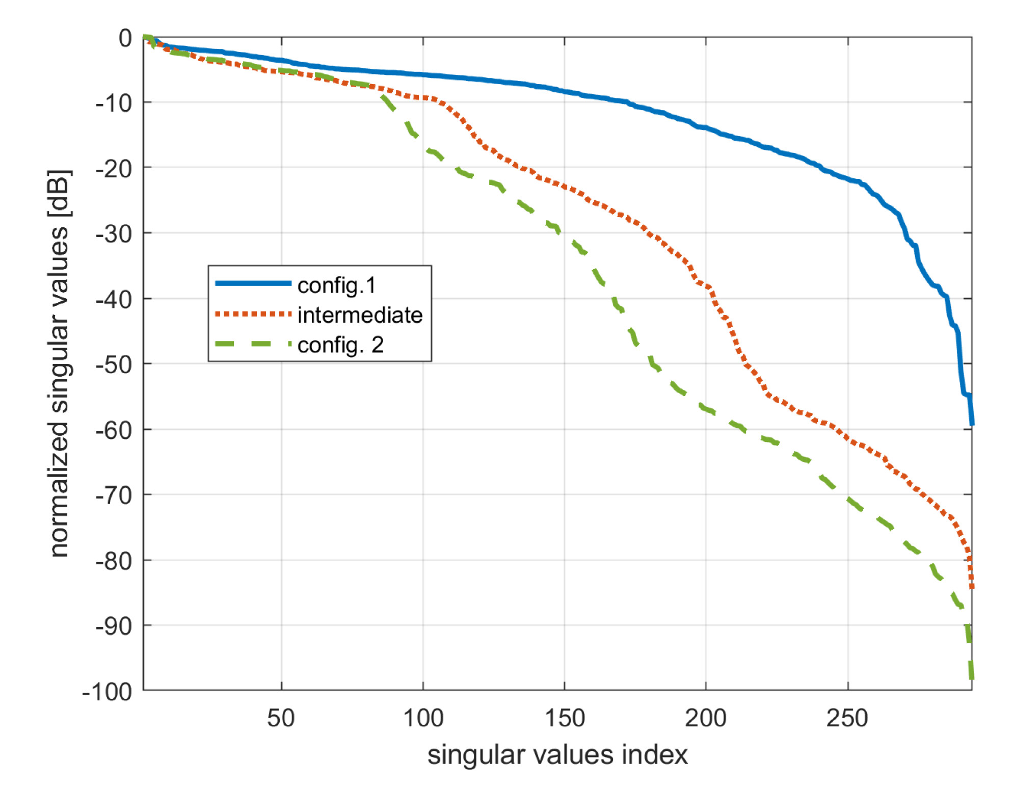
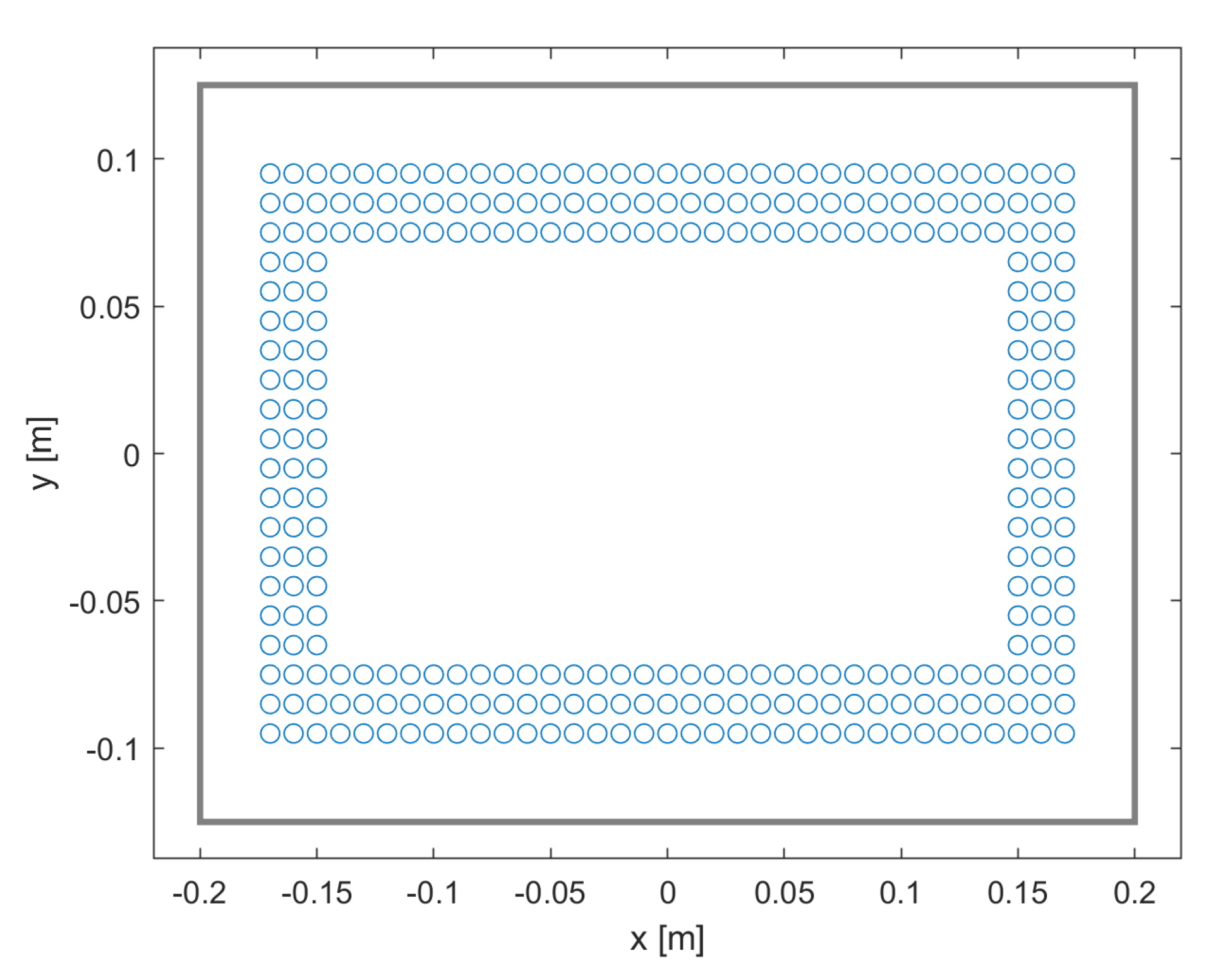
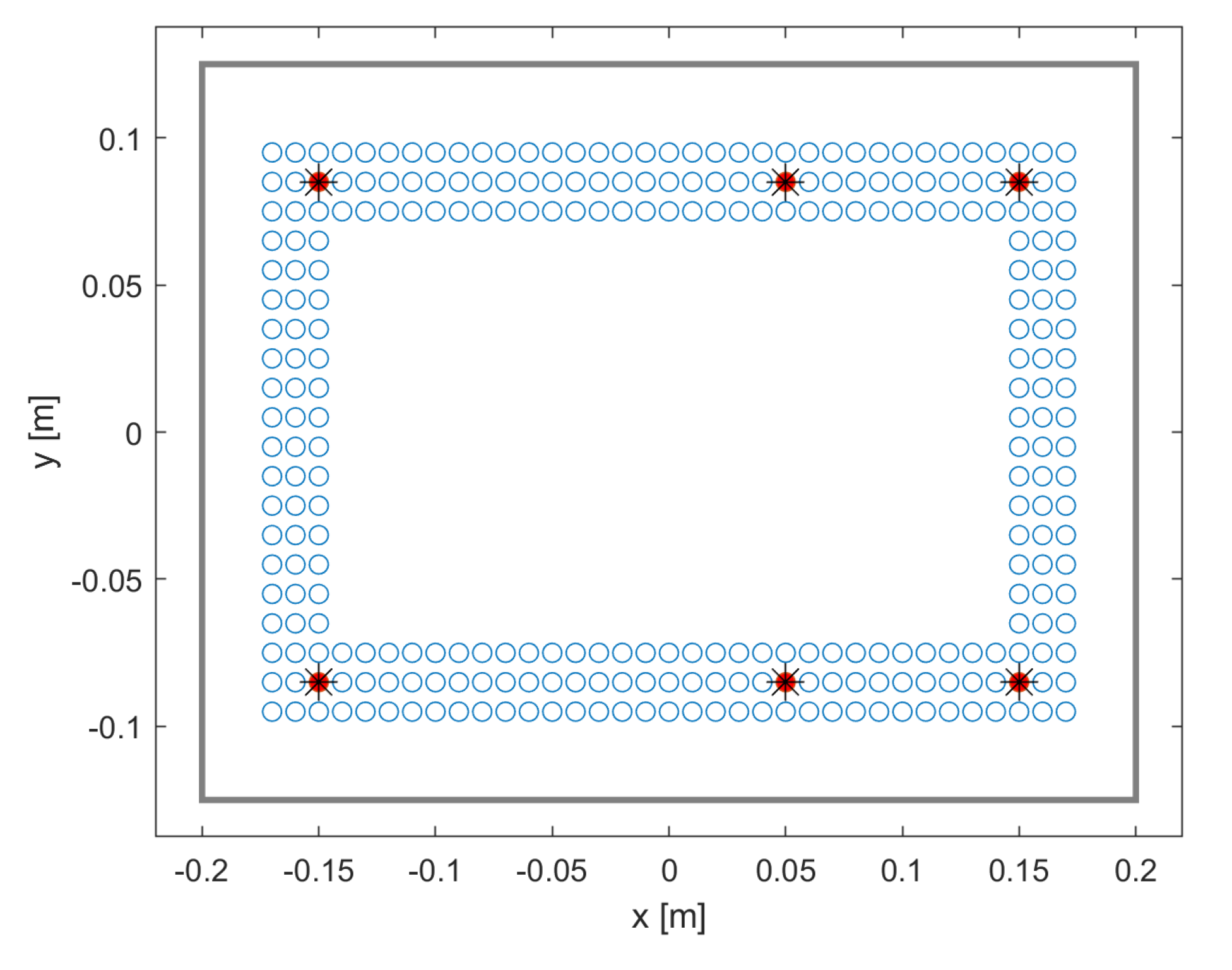
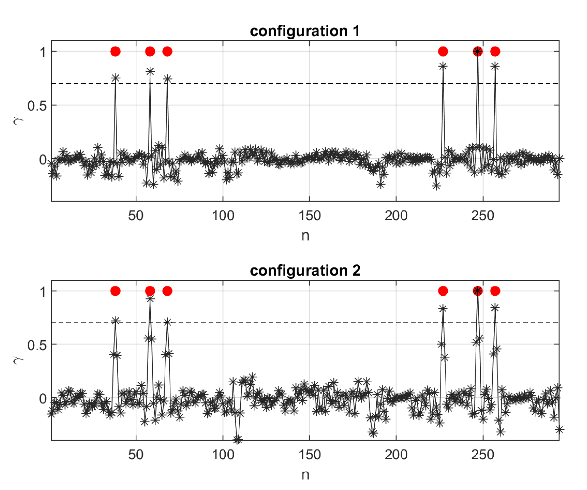
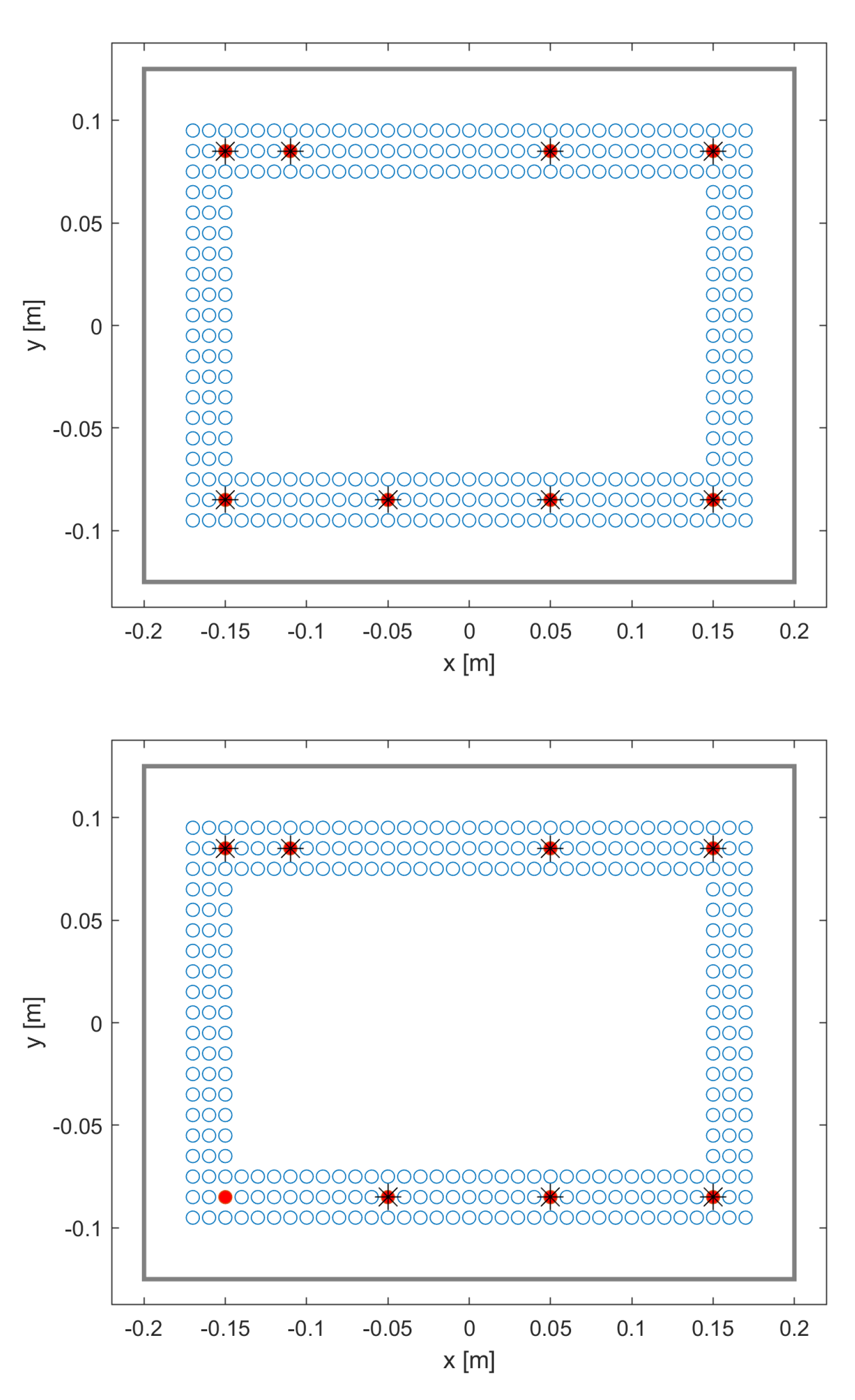
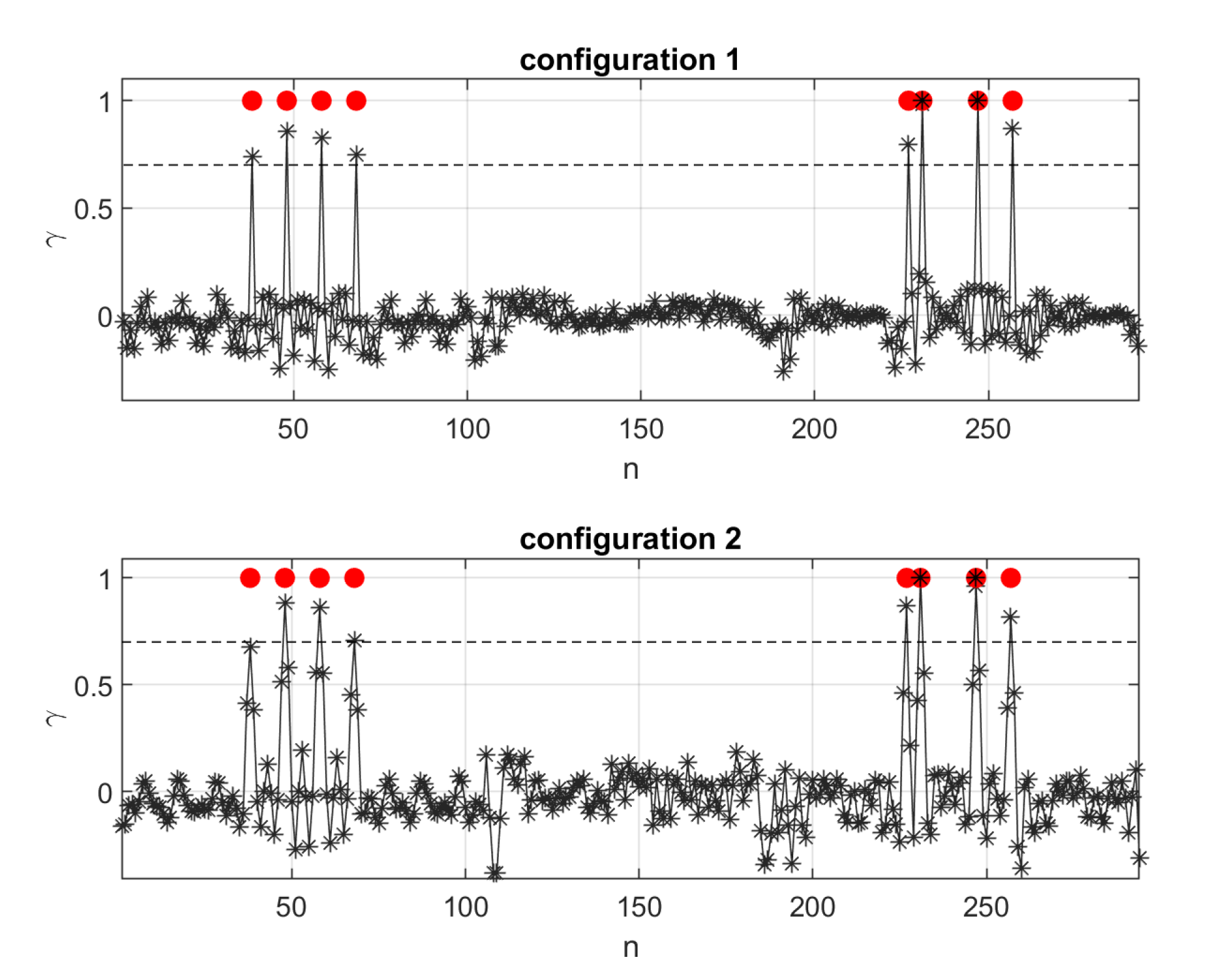
4. Numerical Results

The numerical examples refer to a rectangular investigation domain $\mathsf{\Omega }$, as shown in Figure 1, whose parameters are reported in Table 1 and Table 2. The measurement line is centered with respect to the dielectric rectangle. The data were simulated using the same model developed to perform the inversion and then corrupted by additive Gaussian noise. The signal-to-noise ratio $SNR=20$ dB has been adopted.

First, to appreciate the role of the measurement configuration, the behavior of the singular values for different values of the geometrical and measurement configuration parameters is shown. Two different bandwidths and two different distances between the measurement line and dielectric have been considered. Note that Table 1 refers to the frequency f related to the wavenumber $k=2\pi f/c_0$ where $c_0=3·{10}^8$ m/s. Matrix $\mathbf{G}$ and its TSVD were calculated for the geometry and parameters defined in Table 1 and Table 2. The singular values for the two configurations specified in Table 1 are shown in Figure 3, where the blue line refers to configuration 1, the green line to configuration 2, and the behavior of the singular values obtained when $f_{max}=5$ GHz and $D=0.10$ m is shown by the red line. It can be seen that a wider bandwidth and the enlargement of the angle of view (obtained by moving the measurement line closer to the dielectric while keeping its length fixed) provide better behavior of the singular values, which decay after a larger index. This result is expected and is well known. In fact, in the presence of noise in the data, the truncation of the singular values below $-SNR$ is mandatory to obtain stable inversion [25].

Figure 3. Singular values of $\mathbf{G}$ for different measurement configurations. Intermediate configuration uses same D as config. 1 and maximum frequency as config. 2.

Table 1. Measurement configurations (see Figure 1).

Quantity	Symbol	Config. 1	Config. 2
Measurement line distance from the dielectric	D	10 cm	50 cm
Measurement line extent	L	200 cm	200 cm
Number of observation points	$N_o$	101	101
Minimum frequency (wavenumber)	$f_{min}$ ($k_{min}$)	4 GHz ($83.78$ m${}^{-1}$)	4 GHz ($83.78$ m${}^{-1}$)
Maximum frequency (wavenumber)	$f_{max}$ ($k_{max}$)	7 GHz ($146.61$ m${}^{-1}$)	5 GHz ($104.72$ m${}^{-1}$)
Number of frequencies	$N_k$	101	101

Table 1. Measurement configurations (see Figure 1).

Quantity	Symbol	Config. 1	Config. 2
Measurement line distance from the dielectric	D	10 cm	50 cm
Measurement line extent	L	200 cm	200 cm
Number of observation points	$N_o$	101	101
Minimum frequency (wavenumber)	$f_{min}$ ($k_{min}$)	4 GHz ($83.78$ m${}^{-1}$)	4 GHz ($83.78$ m${}^{-1}$)
Maximum frequency (wavenumber)	$f_{max}$ ($k_{max}$)	7 GHz ($146.61$ m${}^{-1}$)	5 GHz ($104.72$ m${}^{-1}$)
Number of frequencies	$N_k$	101	101

Table 2. Bar and dielectric parameters.

Quantity	Symbol	Value
$\mathsf{\Omega }$ size along x	W	0.40 m
$\mathsf{\Omega }$ size along y	P	0.25 m
Dielectric contrast	$\chi$	3
bars’ conductivity	$\sigma$	${10}^7$ S/m
bars’ radius	a	$8·{10}^{-3}$ m
bars’ candidate number	$N_b$	294 (see Figure 4)

Figure 4. Candidate (blue circles) bar positions inside the dielectric rectangle (grey line). Bars are numbered from bottom left to top right.

Table 2. Bar and dielectric parameters.

Quantity	Symbol	Value
$\mathsf{\Omega }$ size along x	W	0.40 m
$\mathsf{\Omega }$ size along y	P	0.25 m
Dielectric contrast	$\chi$	3
bars’ conductivity	$\sigma$	${10}^7$ S/m
bars’ radius	a	$8·{10}^{-3}$ m
bars’ candidate number	$N_b$	294 (see Figure 4)

To illustrate how the algorithm works, four deployments of the bars have been considered among the $N_b=294$ positions depicted in Figure 4. The different deployments, shown in Figure 5, Figure 6, Figure 7, Figure 8 represent cases in which the bars are regularly spaced and cases in which some bars are out of place or completely lacking. Based on the noise level of the data, a truncation value of $-20$ dB was adopted in the TSVD procedure. Concerning Figure 3, this truncation level corresponds to retaining the first 112 singular values in the “worst” configuration (green line) and the first 241 in the “best” one (blue line). It should be emphasized that the number of singular values above the threshold does not depend on the actual deployment of the bars inside the structure. The corresponding results in terms of detection and localization are shown in Figure 5, Figure 6, Figure 7 and Figure 8. In all figures, the bars are numbered from the bottom left to the top right. Each figure shows a pictorial view of the reconstruction, obtained after thresholding, at the top, and the reconstructed function $\gamma \left(n\right)$ at the bottom. As can be seen, when the number of retained singular values is higher, the bars are successfully detected. In fact, in this case, the recovered function exhibits a very clear behavior, which makes the procedure insensitive to the choice of threshold. In contrast, in the case of a lower number of singular values, some of the bars are not detected, and the choice of the threshold becomes crucial. Moreover, a lower threshold level causes the detection of false bars.

Figure 5. Bars’ detection (top) and reconstructed $\gamma \left(n\right)$ for the two measurement configurations (bottom). Red circles represent actual bars. Black stars represent detected bars. A threshold of $0.7$ has been applied.

Figure 6. Bars’ detection (top) and reconstructed $\gamma \left(n\right)$ for the two measurement configurations (bottom). Red circles represent actual bars (two bars lacking with respect to Figure 5). Black stars represent detected bars. A threshold of $0.7$ has been applied.

Figure 7. Bars’ detection (top) and reconstructed $\gamma \left(n\right)$ (bottom). Red circles represent actual bars (one bar is displaced with respect to Figure 5). Black stars represent detected bars. A threshold of $0.7$ has been applied.

Figure 8. Bars’ detection (configuration 1 and 2 from top) and reconstructed $\gamma \left(n\right)$ (bottom). Red circles represent actual bars. Black stars represent detected bars. A threshold of $0.7$ has been applied. Note the the two lateral bars are not detected in configuration 2.

5. Conclusions

In this study, an approximated model for the scattering from metallic bars embedded into a dielectric is proposed. The model is “quasi” quadratic because it exploits a quadratic approximation of the scattering, which allows the coupling between the bars and the dielectric structure to be taken into account, but it neglects the coupling between the bars. In this way, by exploiting a priori knowledge of the dielectric permittivity and shape, the detection and localization of the bars are reduced to the inversion of a linear operator. The behavior of the singular values of the operator provides indications about the information content of the different measurement configurations. Two examples have been considered. As expected, a wider angle of view (provided in the above examples by bringing the measurement line closer to the dielectric) corresponds to an increased number of singular values above the threshold. The threshold can be fixed according to the expected signal-to-noise ratio of the data, and TSVD guarantees the stability of the inversion algorithm. The proposed model allows for the computation of part of the relevant operator in a closed form so that it reduces the computational burden. The algorithm was validated with numerically simulated data relating to two measurement configurations and different numbers and positionings of the bars inside the dielectric. The results show the feasibility of the approach and encourage a deeper understanding of the model. The application that is considered by the author is reinforced concrete diagnostics. It is worth noting that one of the difficulties in reinforced concrete diagnostics stands in setting up a reliable measurement system, in which the instrumentation’s accurate positioning and the minimization of measurement noise play a crucial role. From this point of view, the availability of simple and stable data processing algorithms is helpful. Experimental validation was not within the scope of this paper. However, a laboratory set-up is in progress in order to obtain the data needed to test the method with experimental measurements performed in a controlled environment.

References

- Pastorino, M.; Randazzo, A. Microwave Imaging Methods and Applications; Artech House: Boston, MA, USA, 2018; ISBN 978-1-63081-348-2. [Google Scholar]
- Daniels, D.J. Ground Penetrating Radar, 2nd ed.; Daniels, D.J., Ed.; IEEE Radar Sonar and Navigation Series; The Institution of Electrical Engineers: London, UK, 2004. [Google Scholar]
- Catapano, I.; Crocco, L.; Napoli, R.D.; Soldovieri, F.; Brancaccio, A.; Pesando, F.; Aiello, A. Microwave tomography enhanced GPR surveys in Centaur’s Domus—Regio VI of Pompeii. J. Geophys. Eng. 2012, 9, 92–99. [Google Scholar] [CrossRef]
- Benedetto, A.; Pajewsky, L. Civil Engineering Applications of Ground Penetrating Radar; Springer: Cham, Switzerland, 2015; ISBN 978-3-319-04813-0. [Google Scholar]
- Catapano, I.; Gennarelli, G.; Ludeno, G.; Noviello, C.; Esposito, G.; Soldovieri, F. Contactless Ground Penetrating Radar Imaging: State of the Art, Challenges, and Microwave Tomography-Based Data Processing. IEEE Geosci. Remote. Sens. Mag. 2021, 10, 251–273. [Google Scholar] [CrossRef]
- Wai-Lok Lai, W.; Dérobert, X.; Annan, P. A review of Ground Penetrating Radar application in civil engineering: A 30-year journey from Locating and Testing to Imaging and Diagnosis. NDT E Int. 2018, 96, 58–78. [Google Scholar] [CrossRef]
- Soldovieri, F.; Brancaccio, A.; Prisco, G.; Leone, G.; Pierri, R. A Kirchhoff-based shape reconstruction algorithm for the multimonostatic configuration: The realistic case of buried pipes. IEEE Trans. Geosci. Remote Sens. 2008, 46, 3031–3038. [Google Scholar] [CrossRef]
- Aboudourib, A.; Serhir, M.; Lesselier, D. A processing framework for tree-root reconstruction Using ground-penetrating radar Under heterogeneous soil conditions. IEEE Trans. Geosci. Remote Sens. 2021, 59, 208–219. [Google Scholar] [CrossRef]
- Brancaccio, A.; Leone, G.; Solimene, R. Fault detection in metallic grid scattering. J. Opt. Soc. Am. A 2011, 28, 2588–2599. [Google Scholar] [CrossRef]
- Brancaccio, A.; Solimene, R. Fault detection in dielectric grid scatterers. Opt. Express 2015, 23, 8200–8215. [Google Scholar] [CrossRef]
- Pichot, C.; Trouillet, P. Diagnosis of reinforced structures: An active microwave imaging system. In Bridge Evaluation, Repair and Rehabilitation; Nowak, A.S., Ed.; NATO ASI Series (Series E: Applied Sciences); Springer: Dordrecht, The Netherlands, 1990; Volume 187, pp. 201–215. [Google Scholar] [CrossRef]
- Leucci, G. Electromagnetic monitoring of concrete structures. In Proceedings of the XIII International Conference on Ground Penetrating Radar, Lecce, Italy, 21–25 June 2010; pp. 1–5. [Google Scholar] [CrossRef]
- Polimeno, M.R.; Roselli, I.; Luprano, V.A.M.; Mongelli, M.; Tatì, A.; Canio, G.D. A non-destructive testing methodology for damage assessment of reinforced concrete buildings after seismic events. Eng. Struct. 2018, 163, 122–136. [Google Scholar] [CrossRef]
- Chun, P.-j.; Hayashi, S. Development of a Concrete Floating and Delamination Detection System Using Infrared Thermography. IEEE/ASME Trans. Mechatron. 2021, 26, 2835–2844. [Google Scholar] [CrossRef]
- Bektaş, Ö.; Kurban, Y.C.; Özboylan, B. Development of magnetic flux leakage device as a non-destructive method for structural reinforcement detection. Mater. Construcción 2022, 72, e273. [Google Scholar] [CrossRef]
- Tamhane, D.; Patil, J.; Banerjee, S.; Tallur, S. Feature Engineering of Time-Domain Signals Based on Principal Component Analysis for Rebar Corrosion Assessment Using Pulse Eddy Current. IEEE Sens. J. 2021, 21, 22086–22093. [Google Scholar] [CrossRef]
- Minutolo, V.; Cerri, E.; Coscetta, A.; Damiano, E.; Cristofaro, M.D.; Gennaro, L.D.; Esposito, L.; Ferla, P.; Mirabile, M.; Olivares, L.; et al. NSHT: New smart hybrid transducer for structural and geotechnical applications. Appl. Sci. 2020, 10, 4498. [Google Scholar] [CrossRef]
- Bernini, R.; Fraldi, M.; Minardo, A.; Minutolo, V.; Carannante, F.; Nunziante, L.; Zeni, L. Identification of defects and strain error estimation for bending steel beams using time domain Brillouin distributed optical fiber sensors. Smart Mater. Struct. 2006, 15, 612–622. [Google Scholar] [CrossRef]
- Karahan, Ş.; Büyüksaraç, A.; Işık, E. The Relationship between Concrete Strengths Obtained by Destructive and Non-destructive Methods. Iran. J. Sci. Technol. Trans. Civ. Eng. 2020, 44, 91–105. [Google Scholar] [CrossRef]
- Marchisotti, D.; Zappa, E. Feasibility Study of Drone-Based 3-D Measurement of Defects in Concrete Structures. IEEE Trans. Instrum. Meas. 2022, 71, 5010711. [Google Scholar] [CrossRef]
- Giannakis, I.; Giannopoulos, A.; Warren, C. A Machine Learning Scheme for Estimating the Diameter of Reinforcing Bars Using Ground Penetrating Radar. IEEE Geosci. Remote Sens. Lett. 2021, 18, 461–465. [Google Scholar] [CrossRef]
- Dinh, K.; Gucunski, N.; Duong, T.H. Migration-based automated rebar picking for condition assessment of concrete bridge decks with ground penetrating radar. NDT E Int. 2018, 98, 45–54. [Google Scholar] [CrossRef]
- Tricomi, F.G. Integral Equations; Interscience Publisher: New York, NY, USA, 1970. [Google Scholar]
- Kantorovich, L.V.; Akilov, G.P. Functional Analysis; Pergamon Press: Oxford, UK, 1982. [Google Scholar]
- Bertero, V.; Boccacci, P. Introduction to Inverse Problems in Imaging; IOP: Bristol, UK, 1998. [Google Scholar]
- Pastorino, M. Microwave Imaging; Wiley Series in Microwave and Optical Engineering; John Wiley and Sons: Hoboken, NJ, USA, 2018; ISBN 9780470602478. Available online: https://books.google.it/books?id=uiObPresrM0C (accessed on 1 March 2022).
- Bevacqua, M.T.; Isernia, T. Quantitative Non-Linear Inverse Scattering: A Wealth of Possibilities Through Smart Rewritings of the Basic Equations. IEEE Open J. Antennas Propag. 2021, 2, 335–348. [Google Scholar] [CrossRef]
- Pierri, R.; Brancaccio, A. Imaging of a rotationally symmetric dielectric cylinder by a quadratic approach. J. Opt. Soc. Am. A 1997, 14, 2777–2785. [Google Scholar] [CrossRef]
- Leone, G.; Brancaccio, A.; Pierri, R. Linear and quadratic inverse scattering for angularly varying circular cylinders. J. Opt. Soc. Am. A 1999, 16, 2887–2895. [Google Scholar] [CrossRef]
- Brancaccio, A. Localization of bars in reinforced concrete by microwaves: A quasi-quadratic inverse scattering approach. In Proceedings of the 2021 XXXIVth General Assembly and Scientific Symposium of the International Union of Radio Science (URSI GASS), Rome, Italy, 28 August–4 September 2021; pp. 1–3. [Google Scholar] [CrossRef]
- Brancaccio, A.; Pascazio, V.; Pierri, R. A quadratic model for inverse profiling: The one-dimensional case. J. Electromagn. Waves Appl. 1995, 9, 673–696. [Google Scholar] [CrossRef]
- Maisto, M.A.; Masoodi, M.; Leone, G.; Solimene, R.; Pierri, R. Scattered Far-Field Sampling in Multi-Static Multi-Frequency Configuration. Sensors 2021, 21, 4724. [Google Scholar] [CrossRef] [PubMed]
- Brancaccio, A.; Leone, G.; Pierri, R. Information content of Born scattered fields: Results in the circular cylindrical case. J. Opt. Soc. Am. A 1998, 15, 1909–1917. [Google Scholar] [CrossRef]
- Abramowitz, M.; Stegun, I.A. Handbook of Mathematical Functions, 9th ed.; U.S. Government Printing Office: Washington, DC, USA, 1970; pp. 358–433.
- Gradshteyn, I.S.; Ryzhik, I.M. Table of Integrals, Series, and Products, 7th ed.; Jeffrey, A., Zwillinger, D., Eds.; Elsevier: Burlington, MA, USA, 2007; pp. 629–630. [Google Scholar]
- Errata for Tables of Integrals, Series, and Products (8th Edition). p. 21, Formula n. 63. Available online: http://www.mathtable.com/errata/gr8_errata.pdf (accessed on 1 March 2022).
Publisher’s Note: MDPI stays neutral with regard to jurisdictional claims in published maps and institutional affiliations. |
© 2022 by the author. Licensee MDPI, Basel, Switzerland. This article is an open access article distributed under the terms and conditions of the Creative Commons Attribution (CC BY) license (https://creativecommons.org/licenses/by/4.0/).