Orientation and Exposure Efficiency of a Solar Tracking Surface in Clear Sky

Abstract

With regard to the problem of current solar irradiation of the tracking surface by the tracker, this can be rationally assessed using a modeled flux with parameters close to the natural direct in accordance with the maximum transparent atmosphere. As part of the experimental research, the values of the air optical mass index in the zenith angle ranging from 0° to 90° were presented for the surface at sea level. The conducted analysis made it possible to confront the experimental research with the models of the optical air transparency mass index. In order to maximize the energy of the controlled beam of the sun’s rays, the angle of their incidence on the tracking surface by the tracker should be minimized. The modeling results show the actual hourly dependencies, which are average values of the intensity of the multi-year measurement. It was found that seasonal dependencies can be considered as theoretically possible and then used to assess the energy efficiency of the tracking surface. Theoretically, they also correspond to the maximum possible energy efficiency of continuous tracking of the Sun with a two-axis rotary tracker. A polar-rotary tracker is a device where the axis of rotation is parallel to the axis of the earth and orients the tracking surface using the simplest synchronous algorithm with a constant angular speed ω = 15 grad/h. The novelty of the article is a method presenting the combination of a normal trajectory with direction towards the sun. Due to the deviation towards the polar axis, the normal touches the horizon, not at six hours after full sun, but earlier and simultaneously. In this way, an uniaxial pole-rotating tracker provides the same irradiation regime as a biaxial one in terms of the deviation of the tracking surface from the axis of rotation, which is equal to the tilt of the sun.

1. Introduction

Among the known renewables, the most commonly explored and widely used is solar energy, which is energy generated from the power of the solar radiation. This is the cleanest method of energy production and the less harmful to our climate [1]. Due to its sustainability and endless resources, it can be called “completely green energy”. Besides its clear advantages, solar energy presents some drawbacks, which are mainly due to its very nature. In different places in the world we can count on various ratios of sunny hours, and even in the hottest places in the world it is difficult to capture enough solar energy to be able to convert it to be used in technological applications. For example, it was found that most solar panels have a relatively low efficiency, which is less than 40% [2]. In order to increase the efficiency of solar panels, technologists and researchers developed the approach of solar tracking.

A solar tracker is a device which ensures maximum intensity of the sun’s rays at the surface of the installed solar panel over time [2]. This system, in order to increase the energy collected from direct irradiance, which is of the highest intensity, moves the photovoltaic panels to orient them perpendicular to the sun’s rays. Over the years, plenty of models have been developed and an intense and continuous increase in interest in solar tracking technology is visible in the literature [3,4,5,6,7].

A team of researchers led by Xinhong [3] claims that generating electricity using solar energy is inefficient. They carried out a project focusing on how to improve the efficiency of solar panels. The researchers found that the solar panel receives the most sunlight when it is perpendicular to the sun’s rays, but that sunlight changes direction regularly with changing seasons and weather. Today, most solar panels are repaired, i.e., the solar panel has a fixed orientation to the sky and does not rotate to follow the sun. To increase the illumination of a unit area by sunlight on solar panels, they are designed to track the production of electricity by the sun. The design mechanism holds the solar panel and enables the panel to perform an approximate three-dimensional (3-D) hemispherical rotation to track the sun’s movement throughout the day and improve overall electricity production. This system can achieve maximum lighting and energy concentration and lower electricity costs by requiring fewer solar panels, so it is of great importance for research and development.

Another research project [4] is for a tracking app for self-tracking 3 kW solar energy off-grid, i.e., a concentrated solar energy system. This sun tracker app uses sunlight in a Stirling system or concentrated PV system by implementing a dynamic mechatronic platform and digital electronic control system to autonomously concentrate solar energy. The solar tracker uses Siemens Solar Library’s Solar function block on Siemens Simatic industrial logic programmable logic TIA microcontroller platform (PLC), remotely monitored by Siemens Simatic iOS S7-1200 application for iPhone/iPad. The project meets the goal of providing a high-precision dynamic solar tracking mobile platform for a concentrated solar power system that is easy to transport, assemble and install over a rural area. Real-time experiments monitored with the Arduino PIC processor show that the implemented solar tracker project performs continuous tracking of sunlight with high optical accuracy.

IoT (Internet of Things) has become a separate research field since the development of internet technology and other communication media [5]. IoT optimizes several tools such as sensor media radio frequency identification, wireless sensor networks and other smart objects that allow humans to easily interact with all devices connected to the internet network. The purpose of this research is to build an IoT-based solar cell tracker which can be controlled through mobile Apps so the data can be read anywhere as long as there is an internet network. The results of this study indicate that the voltage value generated by a dynamic solar cell tracker is greater than that of the static solar cell tracker. Dual axis sun tracker devices that are built using four LDRs produce an average voltage of 19.40 Volt in sunny weather, 18.05 Volt in cloudy weather and 13.60 Volt in rainy weather.

Solar dishes that are formed from a plurality of reflective solar panels are commonly employed for concentrating solar energy and directing this energy to a power conversion unit that converts the solar energy into mechanical and/or electrical energy [6]. A typical power conversion unit has a solar receiver which is positioned relative to the solar dish so as to receive the concentrated solar energy reflected by the solar panels. During the operation of the power conversion unit, it is highly desirable that an even flux be maintained on the receiver so as to increase its service life and ensure efficient operation. Variances in the flux transmitted to the receiver are relatively common and generally result from tracking variation and reflective surface variation. Tracking variation is associated with the positioning of the solar dish and generally results from the control interval that is employed to periodically reposition the solar dish, axis tilts, winds, gravity bending, mirror soiling and track errors. Reflective surface variation is associated with the concentrated light that is reflected by the solar panels and generally results from surface waviness, variation in the radius of curvature and the alignment of the facets (solar panels).

Solar energy is abundant in nature and its sustainable energy resources are present all around the world. The main challenge with the solar field is the lesser amount of solar energy captured by photovoltaic (PV) systems [7]. Great performance of the PV systems can be achieved if the panel is kept perpendicular to the direction of the radiation of the sun. Hence, a solar tracker system is a method to maintain the optimum position of the PV panel always perpendicular to the solar radiation. This paper aims to review various technologies of solar tracking to determine the best PV panel orientation. The various types of technologies for solar tracking systems are discussed, which include a passive solar tracker, active solar tracker and chronological tracker system. The movement degrees of solar tracking systems have also been addressed, consisting of a single-axis solar tracking system and a dual-axis solar tracking system. This paper also overviews tracking techniques, performance, construction, advantages and disadvantages of existing solar tracking systems. The limitations of solar tracking systems are also highlighted for future improvement. Through this research, the most favorable solar tracking system was identified as the active solar tracker with dual axis rotation.

The most important parameters that are crucial for determining optimal position of solar tracking systems are solar irradiance, solar azimuth angle, elevation angle, inclination angle, declination angle and zenith angle, which are used for solar tracking modelling [8]. These systems can be classified into three main categories: passive solar trackers, active solar trackers and chronological solar trackers, based on the techniques that are applied for controlling solar panel movement.

Passive solar tracking systems use non-expensive materials that are thermally active, which means that they can expand with the temperature change, rotating a surface of the panel perpendicularly to the sun. There are available technologies utilizing liquid freon [9], aluminium [10] or other shape memory materials [11,12]. This system is simple in operation and does not rely on any mechanical actuators, what makes it very economic. Nevertheless, due to poor precision in perfectly capturing sun radiation, it is still not sufficiently efficient. Another very important factor is the location of the solar tracker installation in order to attain adequate sunlight for sufficient heating [13].

Active solar trackers follow continuously the position of the sun during the day, using sensors [14]. When the sensor detects change in the solar radiation, it will trigger the motor or actuator to move the position of the panel. Depending on their movement technique, these types of trackers can be further categorized into single-axis or double-axis systems [15]. Although this tracking strategy is much more efficient in terms of solar energy capture, the need to use expensive devices makes it less economic and thus less common.

A chronological solar tracking system is based on the times of the changing position of the sun. A solar panel is moved at a fixed speed and angle during the day [16]. This method of sun tracking is relatively efficient energetically, because there is not too big a tracking error and, thus, low energy losses. Several algorithms for this tracking method have been developed, based also on astronomical equations [17,18,19].

There is still need for improvement in solar tracking performance while maintaining availability and low cost. This article solves the problem of optimizing the use of direct solar flux in terms of solar tracking technology performance. A novelty in the article is the presentation of criteria for assessing the effectiveness of the sun tracking system with the help of orientation and exposure, displaying the basic laws of nature.

2. Materials and Method

The performance of solar trackers is judged against criteria that are difficult to compare. The difficulty arises from the variability of the parameters of the solar surface flux, which depend on the weather, season and territorial specificity. The assessment, presented in the literature [20,21,22,23], usually makes a comparison of the obtained energy, relating to the stationary surface or efficiency of active solar energy installations. Besides weather conditions, the results are additionally influenced by constructive peculiarities and exploitation characteristics of energy installations. Trackers are devices necessary to optimize the use of direct solar flux. Hence, it is more objective to compare initial figures, particularly angle of illumination, irradiation and energy exposure, i.e., the amount of energy arriving at the surface per time unit.

The monograph [23] presents hourly dependencies of irradiation of tracking surfaces, separately for each season of a year—summer and winter solstice and equinox. They are calculated for surface flux of standard intensity at latitude 35° and without specification of standard parameters. In contrast, [24] estimates energy irradiation of the surface of discrete orientation in a flux assumption. Its intensity G_b is described by the convenient equation of Kastrov. Equation (1) is as follows:

$$G_b=\frac{G_{sn}}{1+cm}$$

(1)

Constant c agrees with the results of many years’ pf experiments on the intensity of solar beams in a clear sky. Hence, a daily distribution of intensity, adopted for calculation, in both cases is based on statistical average characteristics of natural fluxes of solar energy. This causes dependency of the results of comparison on applied databases.

Results of immediate measuring of energy efficiency of a flat surface under illumination by a natural flux of solar energy always have diffusion and reflection components. Contribution of these components are hardly considered because of the impact of weather-dependent factors on the space distribution of the diffusion flux intensity and elements of relief and cloudiness on a reflected flux. Thus, current irradiation of the tracking surface is reasonably assessed by a modeled flux, with parameters which are close to the natural direct one, according to the maximum transparent atmosphere.

At the entrance of the atmosphere, density (intensity) of the flux of solar energy during a year variates from the maximum 1415 to minimum 1321 W/m² due to ellipticity of the earth’s orbit. Its average value, which is equal to G_sc = 1367 W/m², is called a solar constant and current values for G_sn for any day in a year have a sequence number n; accuracy, appropriate for comparison, can be calculated by the known Equation [21] (2):

$$G_{sn}=G_{sc}\left(1+0.033 cos\frac{360n}{365}\right)$$

(2)

On 21 June (the day of summer solstice), G_sn =1323 W/m²; on 21 March (equinox), it is equal to 1376 watts per square meter; and on 21 December (the day of winter solstice) it is 1412 W/m². The presented values are very close to the average in the same month and, thus, the accordingly calculated parameters of modeled fluxes can be convenient verified with the appropriate results of actinometrical measuring, first by hourly data of direct solar radiation on the surfaces, which are normal to the beams in a clear sky. The corresponding values are presented in meteorological databases, particularly in [25,26], in Ukraine.

In the CI system of optical energy values, the beam energy, received by the surface, is called energy exposure, marked by the letter H and is measured in watts per hour or joules. This value is an integral characteristic of a flux of solar energy, which is practically divided into hour exposure, marked by letter I, and daily exposure, which is marked by H [23]. Presentation of a flux of energy in the form of hourly data is convenient, as its value in watts per hour is numerically equal to the average energy irradiation of the surface in W/m² and to the density (intensity) of a flux of solar energy, which is measured in the same units. Hence, such practically important calculations and simple equations are satisfactory performed. Equation (3) is as follows:

$$I\approx E\Delta \tau \approx G_b cos\theta \Delta \tau$$

(3)

Thus, daily energy exposure is equal to the hourly total: H = ƩI. A current value cosθ features a momentary (orientation) efficiency of the tracking surface, while energy exposure depicts an integral (energy) efficiency. Hence, accordance of a modeled flux to the natural is convenient to compare with actinometrical data, i.e., hourly solar energy, coming to the surface, which is normal to beams in a clear sky.

Under cloudless weather, intensity of surface direct flux of solar energy ceases due to light interaction with the components of air, having mass M on the beam’s direction in the atmosphere. The vertical direction of the air of mass M₀, which can be calculated by the known barometric equation used in physics, is taken as a unit of comparison. Hence, the mass M of an inclined air column is convenient to be manifested by a relative optical mass m = M/M₀. In actinometry, that integral value is called an optical mass, which serves for calculation of air transparency. However, unequal density and unclear definition of the criterion of an upper boundary of the atmosphere cause the value m to be assessed by approximate correlations, depending on physical interpretation of the interaction process.

The simplest correlation between the air mass and length of the inclined air column is obtained for its hydraulic model, i.e., a flat layer of uncompressed liquid above the height H₀. According to the known equations of hydrostatics (4):

$$H_0=\frac{p_0}{{\rho }_{0}g}=\frac{M_0}{{\rho }_{0}gS}$$

(4)

Under the normal air pressure p₀ = 101.325 kPa and temperature 0 °C, density of air on the Earth’s surface ρ₀ = 1293 kg/m³ height H₀ = 7988 m. In that model, the relative atmospheric mass does not depend on pressure and density of air, and under zenith deflection of a beam by the angle θ_z, correlation of the masses is equal to the correlation of lengths and is manifested by the equation for atmospheric mass (AM) (5):

$$m=\frac{M}{M_0}=\frac{H}{H_0}=\frac{1}{cos{\theta }_z}$$

(5)

According to the equation, the value m asymptotically tends to infinity under the Sun approaching the horizon. To overcome this discrepancy, the atmosphere is modeled as a spherical envelope of a homogeneous density outside the globe. Under its inclined illumination, the value m is calculated by the equation, proven by Lambert [27,28] (6):

$$m=\frac{1}{H_0}\left(\sqrt{R^{2}si{n}^{2}h+2R{H}_0+H_0^2}-R sin h\right)$$

(6)

Under normal conditions at sea level, H₀ = 7994 ≈ 8000 m. Under such a geometric model, at the moments of sunrise or sunset h = 0, the value m is limited and does not exceed the maximum 39.9. This serves as a reference while modifying the Equation (4) for assessment of the integral transparency of real atmosphere with non-homogeneous distribution of pressure, temperature, humidity, extension of the trajectory of beams due to refraction, etc. The present work applies a modified equation of Kasten-Jong [29,30,31], recommended by the European Solar Radiation Atlas (ESRA) [32,33] (7):

$$m=\frac{exp \left(-\frac{z}{8334.5}\right)}{cos{\theta }_z+0.50572{\left(96.07995-{\theta }_z\right)}^{-1.6354}}$$

(7)

where 8334.5 is the coefficient corresponding to the altitude, at which the air pressure reduced e = 2.7193 times.

Table 1. Values of air and optical masses by Equations (3) and (5) (own study).

θz	0	10	20	30	40	50	60	70	80	85	88	90
AM	1	1.015	1.064	1.155	1.305	1.556	2.000	2.924	5.759	11.474	28.65	∞
m at z = 0	1	1.015	1.064	1.154	1.304	1.554	1.994	2.902	5.581	10.306	19.51	37.85

presents values of the optical mass of the air in the intervals of zenith angle from 0° to 90°, calculated by Equations (3) and (5) for the surface at sea level. At a change of the altitude of location by 100 m, the value of air mass is approximately reduced by 1.2% and this should be considered while comparing the modeled fluxes of solar energy with natural.

The appropriate graphic dependencies are demonstrated in Figure 1.

In actinometry, air transparency is quantitatively assessed by these parameters, which are dependent on the optical mass along the beam path under conditions of clear sky. According to the peculiarities of interaction with solar beams, atmosphere is divided into ideal and real. Ideal atmosphere consists only of the main gaseous molecules of air components without carbon dioxide, water vapor and aerosols. In the atmosphere, solar beams become weaker due to interaction of light with the molecules of air by two mechanisms, Rayleigh scattering and selective extinction of the waves of a definite length of the solar spectrum by air molecules and their temporary fluctuations. The total effect is estimated by the integral factor of attenuation δ(m), which depends on the optical mass of air on the beam path. Intensity of the surface flux G_b is conventionally described by the equation, similar to the equation of Lambert for optically homogeneous environments [34] (8):

$$G_b=G_{sn}{e}^{-\delta \left(m\right)m}$$

(8)

Similarly to homogeneous transparent environments, the value δ(m) is also called the optical thickness of the air. Hence, in actinometry, the exponent multiplier is called an integral coefficient of air transparency (9):

$$p=e^{-\delta \left(m\right)}=\sqrt[m]{\frac{G_b}{G_{sn}}}$$

(9)

At average latitudes, the perfect model is best manifested by transparency of highland air, and on the plain under penetration of cold and dry arctic air. Previously, it has been numerically defined by the experimentally adopted pyrheliometric equation of Kasten (10):

$${\delta }_p \left(m\right)=\frac{1}{9.4+0.9m}$$

(10)

3. Results

The studies showed that the values calculated by the Equation (10) were significantly underestimated because they were based on low-resolution spectral data. Consequently, the dependency of Rayleigh scattering on the wavelength was overestimated [35]. Thus, the defined optical thickness is additionally marked by the index symbol δ_R(m) and the specified expression for its calculation by a regression equation (exponential function), as for example in the European Solar Radiation Atlas (ESRA) [32,33] Equations (11) and (12):

$$\frac{\mathbf{1}}{{\mathit{\delta }}_{\mathit{R}} \left(\mathit{m}\right)}\mathbf{=}\mathbf{6.6296}\mathbf{+}\mathbf{1.7513}\mathit{m}\mathbf{-}\mathbf{0}\mathbf{,}\mathbf{1202}{\mathit{m}}^{\mathit{2}}\mathbf{+}\mathbf{0.0065}{\mathit{m}}^{\mathit{3}}\mathbf{-}\mathbf{0.00013}{\mathit{m}}^{\mathit{4}}$$

(11)

at m < 20 and h > 1.9°;

$$\frac{\mathbf{1}}{{\mathit{\delta }}_{\mathit{R}} \left(\mathit{m}\right)}\mathbf{=}\mathbf{10.4}\mathbf{+}\mathbf{0.7518}\mathit{m}$$

(12)

at m > 20 and h < 1.9°.

Values of the optical thickness obtained by Equations (10)–(12) are the initial parameters for calculation of practically important optical characteristics of a real atmosphere, i.e., visibility, turbidity, dustiness, etc. However, in both cases, they depend on the optical air mass. Thus, their values, calculated at m = 2, are considered as standard. Choice of the point for comparison is explained by the fact that, at middle latitudes, the Sun never stays at its zenith. Thus, the closest integer value of air mass is chosen for the sake of convenience (Figure 2).

The correlation between them looks like (13):

$$\frac{{\mathit{\delta }}_{\mathit{P}} \left(\mathbf{2}\right)}{{\mathit{\delta }}_{\mathit{R}} \left(\mathbf{2}\right)}\mathbf{=}\frac{\mathbf{0.0893}}{\mathbf{0.1031}}\mathbf{=}\mathbf{0.8662}$$

(13)

and is used as a ratio of proportionality in the working equations for calculation of a direct flux under fixed transparency or vice versa.

Real atmosphere always contains carbon dioxide, water vapor, drops of fog and aerosols. Their total contribution into attenuation of a flux of solar energy is quantitatively assessed by the turbidity factor T(m), which depends on the optical thickness of air. Quantitatively, it is expressed by a non-dimensional value referring to the contribution of the ideal atmosphere, which is taken as a reference unit. The correlations, proposed in literature for dependency on the optical mass of air, are usually additionally indexed by the last names of the author, i.e., T_L—is the Linke turbidity factor; T_LK—is the Kasten turbidity factor, etc. Thus, considering the described specifications, intensity of the surface flux of solar energy is calculated by Equation (8), which, in the case of T_LK(AM2) use, looks like that presented in the ESRA (14):

$$G_b=G_{sn} exp\left[-0.8662{\delta }_R\left(m\right)·T_{LK}\left(AM2\right)m\right]$$

(14)

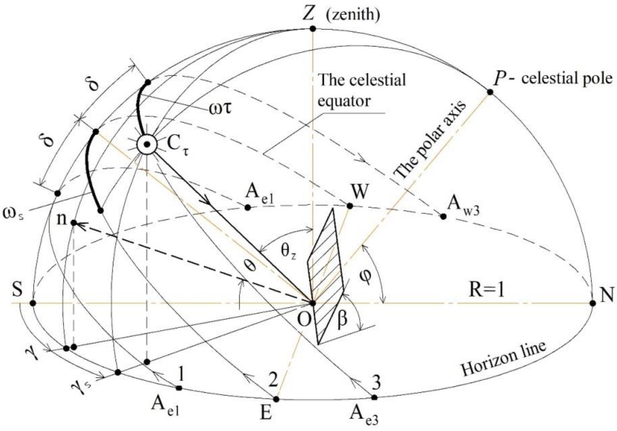
For maximum employment of the energy of controlled flux of solar beams, the angle of their incidence on the tracking surface θ should be minimized. During daylight, the permanent value θ = 0 is secured only by a double-axis rotating device, which is complicated for production and operation. A simpler design is a feature of uniaxial rotating devices that minimize the irradiation angle and only in some cases is this equal to zero. In both variants for optimization of tracking, it is necessary to set analytical correlations between the space-time parameters of a direct flux of solar energy and the receiving surface. The appropriate constructions are performed by the scheme of the Sun irradiation of the surface of a spontaneous orientation, presented in Figure 3, which is based on the concepts and ratios of spherical astronomy [36,37].

The angle space-time parameters of the Sun and of the tracking area are determined in two systems of coordinates, i.e., equatorial, directed along the polar axis OP and horizontal, along the zenith direction OZ. Radius of the conventional globe R is considered as equal to one. Seasonal trajectories of the Sun in the sky are presented for the period of summer and winter solstice and spring equinox. The Sun stays on the surface of a conventional globe and apparently rotates around the polar axis OP, inclined to the surface of horizon at the angle, which is equal to geographical latitude of the area φ. Its day trajectories are marked by three semi-cycles with the centers on the polar axis and correspond to: 1—winter season δ = +23.45°; 2—equinox δ = 0; and 3—summer season δ = −23.45°. The path of equinox coincides with the equinoctial line. Coordinates of the Sun are determined in the equatorial system by the angle δ relating to the equator plane, equal to the seasonal inclination and hour angle ω_s = ω_τ, measured from the southern direction; ω = 15 grad/h is an angle speed of the Earth axial rotation; τ is the hour measured from the moment of full sun. The hour angle is measured along the equinoctial line: on the scheme it is marked by a heavy arc to the cross point with the equatorial vertical, i.e., the arc of a large circle, marked pole of the world, P.

In the horizontal system, the zenith angle θ_z corresponds to the angle of deflection δ, and azimuth of the Sun γ_s corresponds to the hour angle. Graphically, they are defined by the points of intersection of two horizontal verticals (arcs of a large circle, drawn across the zenith) with the line of the horizon. The points of intersection of sun trajectories with the skyline refer to the azimuth of the east A_east and west A_west of the Sun. The tracking surface is placed in the center O of the sky semi-sphere and is inclined at a random angle β to the horizon. Its space orientation is determined by the direction of the normal n and in the horizontal plane by the azimuth deflection γ from the southern direction. The angle of irradiation θ is equal to the angle between the normal and solar beam.

Equatorial and horizontal solar coordinates are interrelated according to the known Equations 15 and 16 of spherical astronomy [36,37], for example:

$$\mathbf{cos}{\mathit{\theta }}_{\mathit{z}}\mathbf{=}\mathit{c}\mathit{o}\mathit{s}\mathit{\phi }\mathit{·}\mathit{c}\mathit{o}\mathit{s}\mathit{\delta }\mathit{·}\mathit{c}\mathit{o}\mathit{s}\mathit{\omega }\mathit{\tau }\mathit{+}\mathit{s}\mathit{i}\mathit{n}\mathit{\phi }\mathit{·}\mathit{s}\mathit{i}\mathit{n}\mathit{\delta }$$

(15)

$$\left|\mathit{c}\mathit{o}\mathit{s}{\mathit{\gamma }}_{\mathit{S}}\right|\mathit{=}\frac{\mathit{c}\mathit{o}\mathit{s}{\mathit{\theta }}_{\mathit{z}}\mathit{·}\mathit{s}\mathit{i}\mathit{n}\mathit{\phi }\mathit{-}\mathit{s}\mathit{i}\mathit{n}\mathit{\delta }}{\mathit{s}\mathit{i}\mathit{n}{\mathit{\theta }}_{\mathit{z}}\mathit{·}\mathit{c}\mathit{o}\mathit{s}\mathit{\phi }} \mathrm{or} \left|\mathit{s}\mathit{i}\mathit{n}{\mathit{\gamma }}_{\mathit{S}}\right|\mathit{=}\frac{\mathit{c}\mathit{o}\mathit{s}\mathit{\delta }\mathit{·}\mathit{s}\mathit{i}\mathit{n}\mathit{\omega }\mathit{\tau }}{\mathit{s}\mathit{i}\mathit{n}{\mathit{\theta }}_{\mathit{z}}}$$

(16)

Moments and directions (azimuths) of the east and west of the Sun are equal in absolute value and opposite by the sign and are measured by Equation (1) at θ_z = 90° as follows (17) and (18):

$$\left|{\mathit{A}}_{\mathit{c}\mathit{x}}\right|\mathit{=}\left|{\mathit{A}}_{\mathit{\epsilon }\mathit{x}}\right|\mathit{=}\mathit{a}\mathit{r}\mathit{c}\mathit{c}\mathit{o}\mathit{s}\frac{\mathit{s}\mathit{i}\mathit{n}\mathit{\delta }}{\mathit{s}\mathit{i}\mathit{n}\mathit{\phi }}$$

(17)

$$\left|{\mathit{\tau }}_{\mathit{c}\mathit{x}}\right|\mathit{=}\left|{\mathit{\tau }}_{\mathit{\epsilon }\mathit{x}}\right|\mathit{=}\frac{\mathbf{1}}{\mathit{\omega }}\mathit{a}\mathit{r}\mathit{c}\mathit{c}\mathit{o}\mathit{s}\left(\mathit{-}\mathit{t}\mathit{g}\mathit{\phi }\mathit{·}\mathit{t}\mathit{g}\mathit{\delta }\right)$$

(18)

The parallel shift of the plane or its normal within the globe almost does not change the angle correlations, due to the much larger radius of the Earth’s orbit. Hence, the angle of irradiation of the surface of spontaneous orientation is calculated by angular dimensions of the Sun, and planes by the known Equation (19):

$$\mathbf{cos}\mathit{\theta }\mathit{=}\mathit{c}\mathit{o}\mathit{s}{\mathit{\theta }}_{\mathit{z}}\mathit{·}\mathit{c}\mathit{o}\mathit{s}\mathit{\beta }\mathit{+}\mathbf{sin}{\mathit{\theta }}_{\mathit{z}}\mathit{·}\mathit{s}\mathit{i}\mathit{n}\mathit{\beta }\mathit{·}\mathit{c}\mathit{o}\mathit{s}\left({\mathit{\gamma }}_{\mathit{s}}\mathit{-}\mathit{\gamma }\right)$$

(19)

In Ukraine, to compare the modeled flux with the natural one, it is convenient to choose coordinates of meteorological stations, which make hourly registration of the flux of solar energy. For instance, at the latitude close to 50°^, there are such stations as “Boryspil”: 50.35° northern latitude and 30.97° eastern longitude and “Kovel”: 51.22° northern latitude and 24.68° eastern longitude, placed at the altitude z = 124 and 172 m above sea level, respectively. Actinometrical observations at the stations are consolidated in two meteorological reference books of 1966 [25] and 1990 [26]. The corresponding orientation values and parameters of a direct surface flux of solar energy at the latitude 50° in clear sky are presented in

Table 2. Angular dimensions of a direct flux of solar energy for the latitude φ = 50°; (own research).

Summer Solstice: δ = 23.45°; τeast/west = ±8.075 h
τ, hour	|ωτ|, grad	θz, grad	cosθz	sinθz	h, grad	sin h	γs, grad	cos γs	sinγs
0	0	26.56	0.8945	0.4471	63.44	0.8945	0	1	0
1	15	29.03	0.8744	0.4852	60.97	0.8744	29.29	0.8721	0.4893
2	30	36.36	0.8155	0.5788	54.64	0.8155	52.42	0.6099	0.7925
3	45	43.80	0.7218	0.6921	46.20	0.7218	69.60	0.3485	0.9373
4	60	53.15	0.5997	0.8002	36.85	0.5997	83.12	0.1198	0.9928
5	75	62.78	0.4574	0.8893	27.22	0.4574	94.77	−0.0832	0.9965
6	90	72.25	0.3048	0.9524	17.75	0.3048	105.6	−0.2686	0.9632
7	105	81.25	0.1522	0.9883	8.75	0.1522	116.4	−0.4446	0.8957
8	120	89.93	0.0100	0.9999	0.0007	0.0010	128.1	−0.6170	0.7869
8.075	121.13	90.00	0.0000	1.0000	0.0000	0.0000	128.25	−0.6198	0.7848
Equinox: δ = 0; τeast/west = ±6.00 h
τ, hour	|ωτ|, grad	θz, grad	cosθz	sinθz	h, grad	sin h	γs, grad	cos γs	sinγs
0	0	50.00	0.6428	0.7660	40.00	0.6428	0	1	0
1	15	51.62	0.6209	0.7839	38.38	0.6209	19.28	0.9439	0.3302
2	30	56.17	0.5567	0.8307	33.83	0.5567	37.00	0.7986	0.6019
3	45	62.97	0.4545	0.8907	27.03	0.4545	52.55	0.6081	0.7939
4	60	71.25	0.3214	0.9469	18.75	0.3414	66.14	0.4045	0.9145
5	75	80.42	0.1664	0.9861	9.58	0.1664	78.40	0.2011	0.9790
6	90	90.00	0.0000	1.0000	0.0000	0.0000	90.00	0.0000	1.0000
Winter solstice: δ = −23.45; τeast/west = ±3.92 h
τ, hour	|ωτ|, grad	θz, grad	cosθz	sinθz	h, grad	sin h	γs, grad	cos γs	sinγs
0	0	73.45	0.2849	0.9586	16.55	0.2849	0	1	0
1	15	74.64	0.2648	0.9643	15.36	0.2648	14.27	0.9692	0.2464
2	30	78.12	0.2059	0.9786	11.88	0.2059	27.81	0.8845	0.4665
3	45	83.56	0.1122	0.9936	6.44	0.1122	40.75	0.7576	0.9373
3.92	58.87	90.000	0	1.0000	0	0	51.75	0.6190	0.7854

and

Table 3. Intensity of direct flux G_b at the latitude 50°; (own research).

τ, Hour	0	1	2	3	4	5	6	7	8	8.075	Σ
Gb(TLK)	Summer solstice Gsn = 1323 W/m2
θz	26.56	29.03	36.36	43.80	53.15	62.78	72.25	81.25	89.93	90	–
cosθz	0.8945	0.8744	0.8155	0.7218	0.5997	0.4574	0.3048	0.1522	0.0100	0	–
z = 124 m	1.1008	1.1126	1.2072	1.3732	1.6399	2.1463	3.2024	6.2218	27.420	37.291	–
δR (m) z = 124 m	0.1188	0.1185	0.1165	0.1133	0.1086	0.1010	0.0892	0.0702	0.0332	0.0269	–
Gb (TLK = 2)	1056	1054	1038	1012	973	910	809	623	275	233	15,244
Gb (TLK = 3)	942	939	918	883	833	753	630	425	124	98	12,778
Gb (TLK = 3.5)	890	887	864	825	771	686	556	352	84	63	11,751
Gb (TLK = 4)	841	838	813	772	714	624	492	291	56	41	10,829
Equinox Gsn = 1376 W/m2
θz	50.00	51.62	56.17	62.97	71.25	80.42	0	–	–	–	–
cosθz	0.6428	0.6209	0.5577	0.4545	0.3214	0.1664	0	–	–	–	–
z = 124 m	1.5302	1.5939	1.7623	2.1590	3.0367	5.6807	19.421	–	–	–	–
δR (m) z =124 m	0.1105	0.1094	0.1066	0.1009	0.0908	0.0788	0.0409	–	–	–	–
Gb (TLK = 2)	1026	1017	994	943	853	634	348	–	–	–	11,282
Gb (TLK = 3)	887	875	844	781	672	430	175	–	–	–	9153
Gb (TLK = 3.5)	824	811	779	711	666	354	124	–	–	–	8414
Gb (TLK = 4)	766	752	718	646	529	292	88	–	–	–	7494
Winter solstice Gsn = 1412 W/m2
θz	73.45	74.64	78.12	83.56	90.00	–	–	–	–	–	–
cosθz	0.2849	0.2648	0.2059	0.1122	0.0000	–	–	–	–	–	–
z = 124 m	3.4151	3.6659	4.6615	8.0113	19.42	–	–	–	–	–	–
δR (m) z = 124 m	0.0873	0.0852	0.0783	0.0635	0.0409	–	–	–	–	–	–
Gb (TL = 2)	842	822	750	585	357	–	–	–	–	–	5846
Gb (TL = 3)	651	627	547	376	179	–	–	–	–	–	4281
Gb(TL = 3.5)	569	548	467	302	127	–	–	–	–	–	3667

Note: the values by Italic type refer to the moment of rise/set of the Sun, which is equal to 3.92 h after full sun in the day of winter solstice.

, respectively.

Table 3 additionally measures daily energy exposure of the surface, standard to the direction of solar beams.

Numerical integration of hourly values is performed by the trapezoidal method with application of the modified equation, for consideration of a symmetric set of data and a time interval for the threshold values less than 1 h.

$$\mathit{H}\mathit{\approx }{\mathit{G}}_{\mathit{n}}{\mathbf{\Delta }}_{\mathit{n}}\mathit{\tau }\mathit{+}{\mathit{G}}_{\mathit{n}\mathit{-}\mathbf{1}}\mathit{+}\mathbf{2}\left({\mathit{G}}_{\mathbf{0}}\mathit{+}{\mathit{G}}_{\mathbf{1}}\mathit{+}\mathit{\cdots }\mathit{+}{\mathit{G}}_{\mathit{n}\mathit{-}\mathbf{2}}\right)\mathbf{\Delta }\mathit{\tau }$$

(20)

where Δτ = 1 h, Δ_nτ = 0.075 h during the summer solstice; Δ_nτ = 0.92winter solstice.

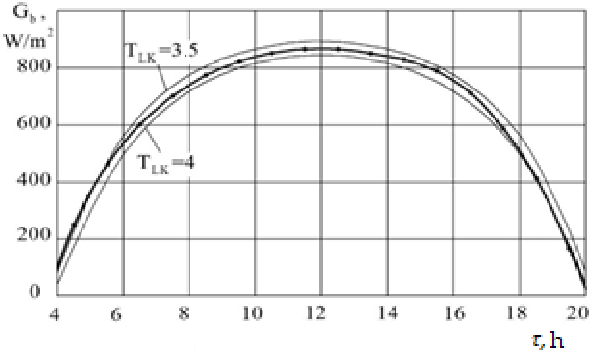
Figure 4 demonstrates hourly data of the energy, registered at the meteorological station “Kovel” in clear sky in June, and presented in watt-hours per square meter. They are depicted by a column diagram and numerically equal values of the flux intensity, in watts per meter square in the form of a continuous dependency, are represented by a thin bypass line. The heavy curve refers to a modeled flux under air turbidity T_LK = 4.

The same comparison of modeled hourly dependencies and those registered at the meteorological station “Boryspil” are demonstrated in Figure 5.

In both cases, results of the modeling satisfactory demonstrate real hourly dependencies, which are average values of the intensity of many years of measurements. It is obvious that small deviations can be explained by local factors of impact on air transparency and random actinometrical criteria when assessing results of measuring and referring to the conditions of clear sky. Hence, energy efficiency of the tracking surface is reasonably calculated at a minimum level of air turbidity T_LK = 2, which meets the requirement of maximum liquidation of the impact of diffusive fluxes on the measuring results. Thus, the seasonal dependencies, presented in Figure 6, can be considered as close as theoretically possible and can be used later for assessment of energy efficiency of the tracking surface. Theoretically, they also correspond to the maximum possible energy efficiency of a continuous tracking of the Sun by means of a double-axis rotating tracker.

Comparison of the daily data of solar energy registered at the meteorological stations “Kovel” and “Boryspil” for the fluxes at different levels of air turbidity are presented in

Table 4. Daily energy exposure of a direct flux on the surface, normal to solar beams (own research).

Databases	Daily Exposure H, W/m2
	Summer Solstice	Spring Equinox	Winter Solstice	Note
Extra-atmospheric flow Gsn	21,366	16,512	11,070	H = Gsn∙τoc (21)
“Kovel” Registered	10,161	8001	4312
“Boryspil” Registered Calculated at:	10,572	8223	3987
TLK = 2	15,244	11,282	5846
TLK = 3	12,778	9153	4281
TLK = 3.5	11,751	8414	3667
TLK = 4	10,829	7494	-

. The values in bold type present the most appropriate values of seasonal natural energy exposures, meeting the conditions of a clear-sky model. Hence, daily solar energy can be considered as the additional integral characteristics of the efficiency of the tracking surface, along with hourly ones. It is clear that hourly and daily energy data, which correspond to the maximum transparency of air T_LK = 2 when one can ignore the diffusive impact on first approaching, are the most reliable and precise characteristics of the energy efficiency of the tracking surface.

4. Discussion

Daily distribution of the intensity of a modeled flux and its integral amount at minimum turbidity of the air should be taken as a theoretically maximum for a double-axis tracker. One-axis rotating trackers, which are less effective, but simpler in production and operation, are classified by orientation of the rotation axis, signified by the name and the short title [23]:

-

a device with a horizontal rotation axis, oriented in the direction “east–west” (horizontal E–W axis tracker—HEW axis tracker);

-

a device with a horizontal rotation axis, oriented in the direction “north–south” (horizontal N–S axis tracker—HNS axis tracker);

-

a device with a vertical rotation axis (vertical axis tracker)—VAT;

-

a device with a polar rotation axis (polar axis tracker)—PAT.

The last two devices expect seasonal optimization of the angle of irradiation by deflection of the tracking surface from the rotation axis, which should be considered while quantitatively assessing their efficiency.

A horizontal rotating device with the rotation axis in the direction “east–west” (HEW) only follows the change in the Sun’s height over the horizon by the scheme presented in Figure 7. The rotating axis is in line with the parallel of the horizontal latitude. Thus, the device should be titled as latitude-rotating. The current maximum of irradiation is achieved under the evident condition that the receiving surface is perpendicular to the plane, drawn across the rotation axis and the Sun, and which contains the triangle BOC.

According to the structure:

$$\mathit{A}\mathit{B}\mathit{=}\mathbf{cos}\mathit{h}\mathit{=}\mathbf{cos}{\mathit{\theta }}_{\mathit{z}}$$

(21)

$$\mathit{O}\mathit{B}\mathit{=}\mathit{A}\mathit{B}\mathit{·}\mathit{s}\mathit{i}\mathit{n} {\mathit{\gamma }}_{\mathit{s}}\mathit{=}\mathit{s}\mathit{i}\mathit{n} {\mathit{\theta }}_{\mathit{s}}\mathit{·}\mathit{s}\mathit{i}\mathit{n} {\mathit{\gamma }}_{\mathit{s}}$$

(22)

$$\mathit{s}\mathit{i}\mathit{n}\mathit{\theta }\mathit{=}\mathit{O}\mathit{B}\mathit{/}\mathit{R}\mathit{=}\mathit{s}\mathit{i}\mathit{n} {\mathit{\theta }}_{\mathit{z}}\mathit{·}\mathit{s}\mathit{i}\mathit{n} {\mathit{\gamma }}_{\mathit{s}}$$

(23)

$$\mathit{c}\mathit{o}\mathit{s}\mathit{\theta }\mathit{=}{\left(\mathbf{1}\mathit{-}\mathit{s}\mathit{i}{\mathit{n}}^{\mathit{2}}\mathit{\theta }\right)}^{\mathbf{0.5}}\mathit{=}{\left(\mathbf{1}\mathit{-}\mathit{s}\mathit{i}{\mathit{n}}^{\mathit{2}}{\mathit{\theta }}_{\mathit{z}}\mathit{·}\mathit{s}\mathit{i}{\mathit{n}}^{\mathbf{2}}{\mathit{\gamma }}_{\mathit{z}}\right)}^{\mathbf{0.5}}$$

(24)

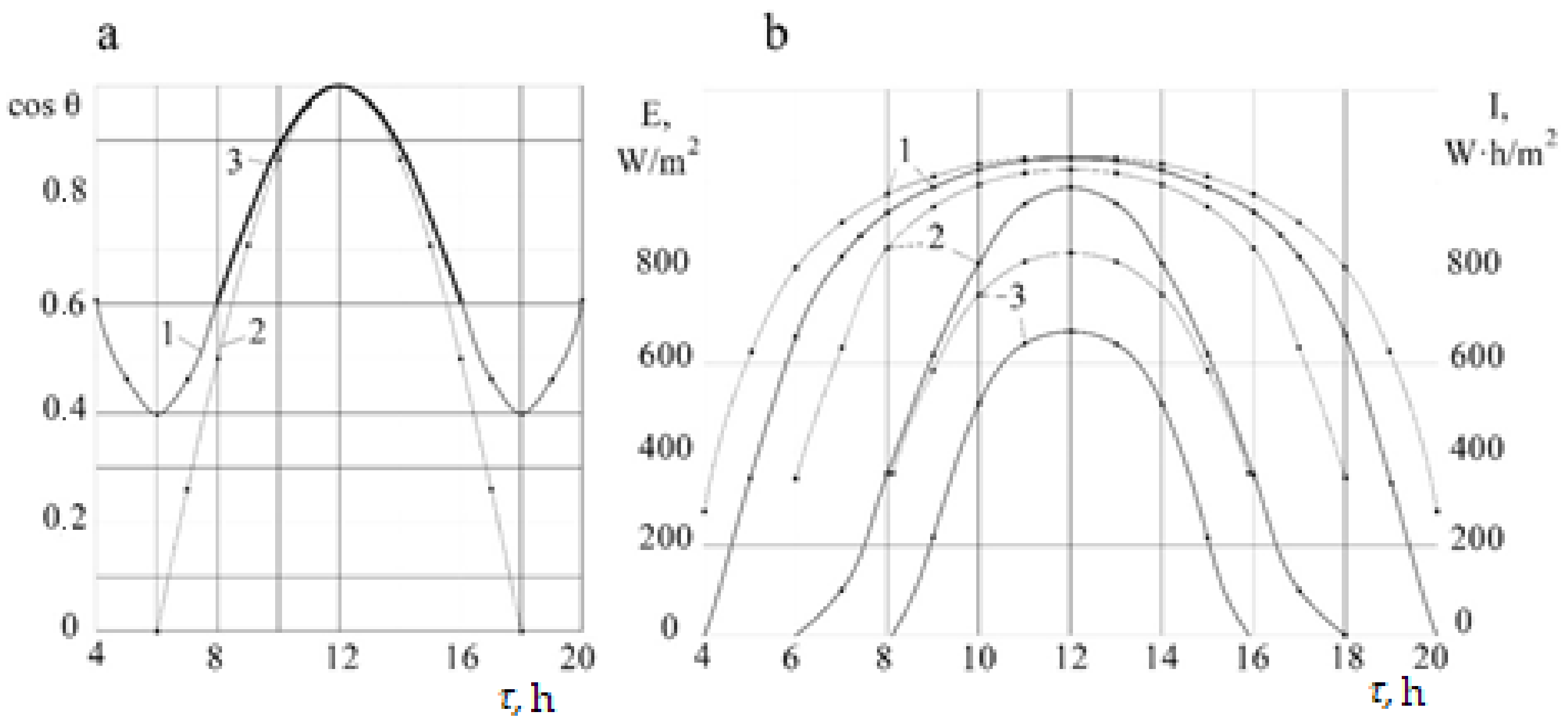
The hourly values cosθ, calculated for the tracking surface by the equation, are presented in

Table 5. Orientation and exposure efficiency of the tracking surface of horizontal axis trackers (own research).

τ, Hour	Summer Solstice Hmax = 15,244 W/d				Spring Equinox Hmax = 11,282 W/d				Winter Solstice Hmax = 5846 W/d
	HWE		HNS		HWE		HNS		HWE		HNS
	cosθ	E, W/m2	cosθ	E, W/m2	cosθ	E, W/m2	cosθ	E, W/m2	cosθ	E, W/m2	cosθ	E, W/m2
0	1	1056	0.8945	945	1	1026	0.6428	660	1	842	0.2849	240
1	0.9714	1024	0.9061	955	0.9659	982	0.6727	684	0.9714	818	0.3557	292
2	0.8886	922	0.9356	971	0.8660	861	0.7483	744	0.8886	666	0.5027	377
3	0.7611	770	0.9705	982	0.7071	667	0.8406	793	0.7071	414	0.6583	385
3.92	–	–	–	–	–	–	–	–	0.5170	185	0.7847	280
4	0.6073	591	0.9954	968	0.5000	427	0.9237	788	–	–	–	–
4.58	0.5190	487	1.0000	939	–	–	–	–	–	–	–	–
5	0.4634	422	0.9972	908	0.2588	164	0.9802	621	–	–	–	–
6	0.3980	322	0.9667	782	0	0	1.0000	348	–	–	–	–
7	0.4634	289	0.8991	560	–	–	–	–	–	–	–	–
8	0.6073	167	0.7945	218	–	–	–	–	–	–	–	–
8.075	0.6191	144	0.5170	120	–	–	1.0000	–	–	–	–	–
H, W∙hours	–	10,971 72.0%	–	14,373 94.3%	–	8254 73.2%	–	8928 79.1%	–	5441 93.1%	–	2509 42.9%

(column HWE) and the corresponding graphical dependencies for cosθ of summer and winter solstice and periods of equinox are demonstrated by Figure 8a. In the period between the spring and autumn equinox, the Sun stays in the northern part of the semi-sphere after the sunrise and before the sunset. To employ the flux of morning and evening periods, it is necessary to change orientation of the receiving surface from southern to northern. Theoretically, this means that twice a day from the moment of transition of the Sun azimuth across the line “east–west”, the azimuth of the tracking surface changes to the opposite one, and on the graphical dependency the decay cosθ is changed into growth.

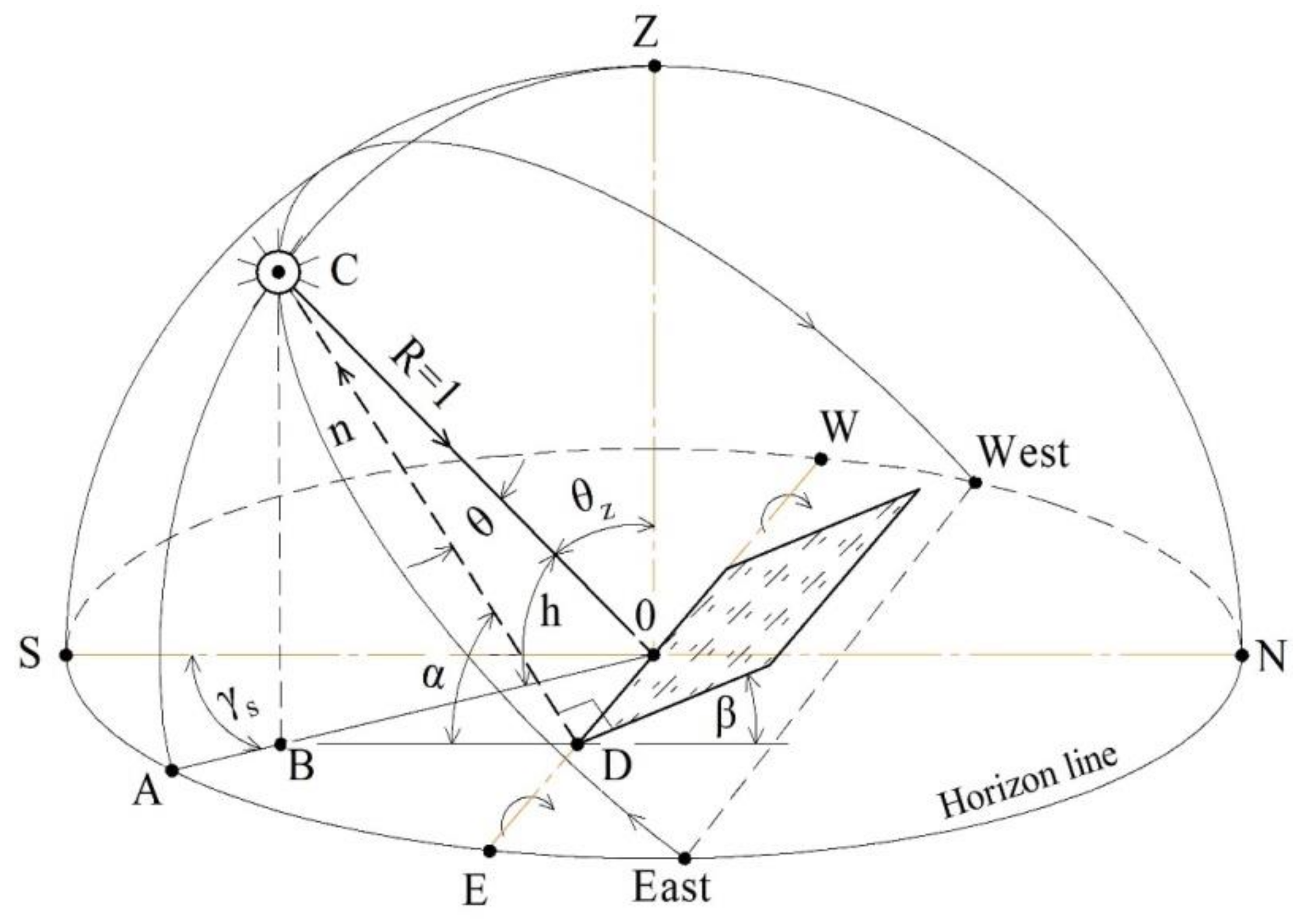
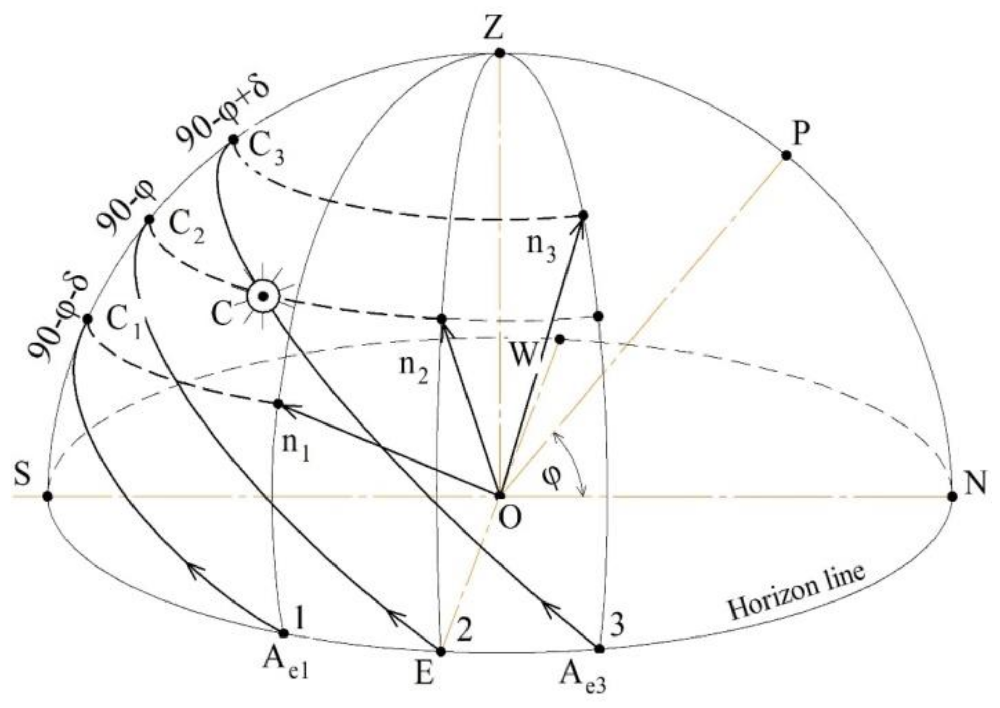
A tracker with a horizontal axis of rotation in the direction “north–south” (HNS axis tracker) follows a daily azimuth path of the Sun from the east to west. The current maximum of irradiation is achieved under the evident condition that the receiving surface is perpendicular to the plane, drawn across the rotation axis, the Sun normal and the surface. The appropriate scheme of irradiation and construction for measuring of the dependency of the angle of inclination and orientation efficiency of the receiving surface for the first half of a day is presented in Figure 9.

According to the construction, the following correlations are performed; particularly a parallel shift of the normal of the tracking surface—the vector $\overrightarrow{n}$—does not change the angular correlations. The current angle of irradiation is determined from the following equations for a right triangle ODC, where D is a right angle:

$$\mathbf{cos}\mathit{\theta }\mathit{=}\frac{\mathit{D}\mathit{C}}{\mathit{R}}\mathit{=}\mathit{D}\mathit{C}$$

(25)

$$\mathit{D}{\mathit{C}}^{\mathit{2}}\mathit{=}\mathit{B}{\mathit{D}}^{\mathit{2}}\mathit{+}\mathit{B}{\mathit{C}}^{\mathit{2}}$$

(26)

$$\frac{\mathit{B}\mathit{C}}{\mathit{R}}\mathit{=}\mathit{s}\mathit{i}\mathit{n} \mathit{h}\mathit{=}\mathbf{cos}{\mathit{\theta }}_{\mathit{z}}$$

(27)

$$\frac{\mathit{O}\mathit{B}}{\mathit{R}}\mathit{=}\mathit{c}\mathit{o}\mathit{s}\mathit{h}\mathit{=}\mathit{sin}{\mathit{\theta }}_{\mathit{z}}$$

(28)

$$\mathit{B}\mathit{D}\mathit{=}\mathit{O}\mathit{B} \mathit{s}\mathit{i}\mathit{n}{\mathit{\gamma }}_{\mathit{s}}\mathit{=}\mathit{s}\mathit{i}\mathit{n} {\mathit{\theta }}_{\mathit{2}}\mathit{s}\mathit{i}\mathit{n}{\mathit{\gamma }}_{\mathit{s}}$$

(29)

hence:

$$\mathbf{cos}\mathit{q}\mathit{=}\sqrt{\mathit{c}\mathit{o}{\mathit{s}}^{\mathit{2}}{\mathit{q}}_{\mathit{z}}\mathit{+}\mathit{s}\mathit{i}{\mathit{n}}^{\mathit{2}}{\mathit{q}}_{\mathit{z}}\mathit{·}\mathit{s}\mathit{i}{\mathit{n}}^{\mathit{2}}{\mathit{\gamma }}_{\mathit{S}}}$$

(30)

or:

$$\mathbf{cos}\mathit{q}\mathit{=}\sqrt{\mathit{c}\mathit{o}{\mathit{s}}^{\mathit{2}}{\mathit{q}}_{\mathit{z}}\mathit{+}\mathit{c}\mathit{o}{\mathit{s}}^{\mathit{2}}{\mathit{q}}_{\mathit{z}}\mathit{·}\mathit{\delta }\mathit{s}\mathit{i}{\mathit{n}}^{\mathit{2}}\mathit{\omega }\mathit{\tau }}$$

(31)

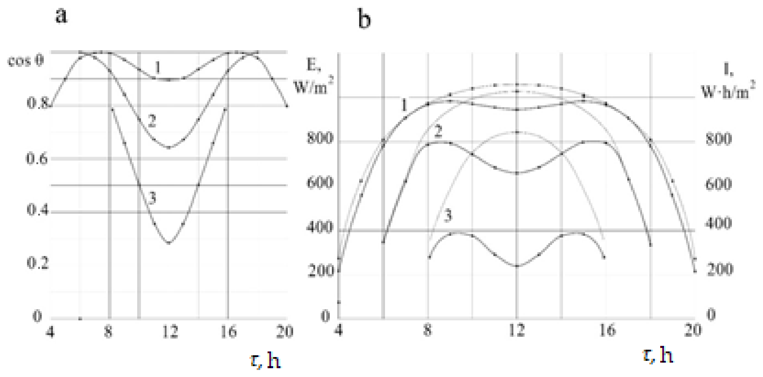
The calculated values cosθ are presented in the column HNS of Table 5 and the corresponding graphical dependencies are demonstrated in Figure 10a.

In the bottom line of Table 5, there are absolute values of daily energy exposures of the tracking surface of both types of horizontal-axis trackers. Percentage efficiency is calculated referring to maximum data of the energy in clear sky, presented in Table 3. In line with the above, it is convenient to estimate the hourly or seasonal efficiency of each period and, if necessary, compare them with the energy efficiency of a stationary space. A vertical-axis rotating tracker secures compensation of the azimuth constituent of a daily path of the Sun in the sky. Its path is demonstrated at Figure 11 and is marked by continuous lines of a standard width.

In contrast, normal of the tracking surface of the permanent inclination outlines the path of the same height over the horizon. On the scheme, they are demonstrated by dash lines and meet the condition of the maximum irradiation at the sunny midday with the inclination angles:

-

in summer:

$$\mathit{\beta }\mathit{=}\mathit{\phi }\mathit{-}{\mathit{23.45}}^{\mathit{o}}\mathit{=}{\mathit{26.55}}^{\mathit{o}}$$

(32)

-

in winter:

$$\mathit{\beta }\mathit{=}\mathit{\phi }\mathit{-}{\mathit{23.45}}^{\mathit{o}}\mathit{=}{\mathit{73.45}}^{\mathit{o}}$$

(33)

-

at equinox:

$$\mathit{\beta }\mathit{=}{\mathit{50}}^{\mathit{o}}$$

(34)

The rest of the day, the minimum angle of irradiation is marked under conditions of equal azimuth angles of the Sun and the rotating surface γ = γ_s. Making its substitution in the Equation (8), one can obtain the following equation for the initial angle of irradiation:

$$\mathbf{c}\mathbf{o}\mathbf{s} \mathit{\theta }\mathit{=}\mathit{c}\mathit{o}\mathit{s}{\mathit{\theta }}_{\mathit{z}}\mathit{c}\mathit{o}\mathit{s}\mathit{\beta }\mathit{+}\mathit{s}\mathit{i}\mathit{n}{\mathit{\theta }}_{\mathit{z}}\mathit{s}\mathit{i}\mathit{n}\mathit{\beta }\mathit{=}\mathit{c}\mathit{o}\mathit{s}\left({\mathit{\theta }}_{\mathit{z}}\mathit{-}\mathit{\beta }\right)$$

(35)

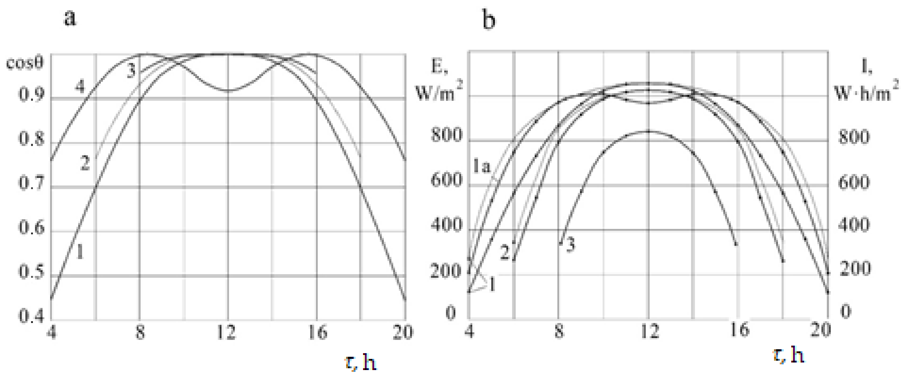
Current values for the above-presented angles of inclination are demonstrated in

Table 6. Orientation and exposure efficiency of the tracking surface while rotating around the vertical axis (own research).

τ, Hour	Summer Solstice				Spring Equinox β = 50°		Winter solst#ice β = φ
	β = φ–δ		β = 50°
	cosθ	E, W∙m2	cosθ	E, W∙m2	cosθ	E, W∙m2	cosθ	E, W∙m2
0	1.0000	1056	0.9175	969	1.0000	1026	1.0000	842
1	0.9991	1053	0.9338	983	0.9996	1017	0.9998	822
2	0.9854	1023	0.9718	1009	0.9942	988	0.9967	748
3	0.9551	966	0.9942	1006	0.9745	919	0.9845	576
3.67	–	–	1.0000	987	–	–	–	–
3.92	–	–	–		–	–	0.9588	342
4	0.8942	870	0.9985	972	0.9320	795	–	–
5	0.8068	734	0.9752	887	0.8623	547	–	–
6	0.6985	565	0.9255	749	0.7660	267	–	–
7	0.5780	360	0.8549	533	–	–	–	–
8	0.4482	123	0.7668	211	–	–	–	–
8.075	0.4471	104	0.7660	178	–	–	–	–
H, W∙hours	–	13,384 87.8%	–	14,440 94.7%	–	10,851 96.2%	–	5715 97.8%

, which have the appropriate graphical dependencies 1, 2, and 3 in Figure 12.

At less angles of inclination, the full sun is characterized by a local minimum of irradiation with two symmetric maximums aside (curve 1b) and increased values cosθ in the rest of the daylight. For instance, at the angle of inclination of the tracking surface β = φ = 50° during summer solstice, trajectory of the “spring” normal n₂ crosses the solar one at 3.67 h: in Figure 12, the point of intersection is marked by a symbol of the Sun.

A polar-rotating tracker is a device, in which the rotating axis is parallel to the earth axis and orients the tracking surface by the simplest synchronic algorithm with a permanent angle speed ω = 15 grad/hour. In the literature, scientists only consider the variant of construction, in which the tracking surface is combined with the rotating axis β = φ. Figure 13 presents the scheme of tracking, which corresponds to the period of equinox, when the end of the normal of a tracking surface traces a common path with the Sun. In its turn, it coincides with the equinoctial line.

In the case of coinciding of the normal with the direction to the Sun, their azimuth angles are equal γ(τ) = γ_s(τ), and orientation efficiency of the surface during a day is permanent and equal to one. The current angle of inclination of the receiving surface is measured by evident equations:

$$\mathbf{A}\mathbf{B} \mathbf{┴}\mathbf{O}\mathbf{B} \mathbf{┴}\mathbf{D}\mathbf{B}$$

(36)

$$\mathit{O}\mathit{A}\mathit{B}\mathit{=}\mathit{\gamma }$$

(37)

$$\mathit{t}\mathit{g}\mathit{\beta }\mathit{=}\frac{\mathit{A}\mathit{D}}{\mathit{A}\mathit{B}}$$

(38)

$$\mathit{A}\mathit{D}\mathit{=}\mathit{A}\mathit{O}\mathit{·}\mathit{t}\mathit{g}\mathit{\phi }$$

(39)

$$\mathit{A}\mathit{B}\mathit{=}\mathit{A}\mathit{O}\mathit{·}\mathit{c}\mathit{o}\mathit{s}{\mathit{\gamma }}_{\mathit{s}}$$

(40)

hence:

$$\mathit{t}\mathit{g}\mathit{\beta } \left(\mathit{\tau }\right)\mathit{=}\frac{\mathit{t}\mathit{g}\mathit{\phi }}{\mathit{c}\mathit{o}\mathit{s}{\mathit{\gamma }}_{\mathit{s}} \left(\mathit{\tau }\right)}$$

(41)

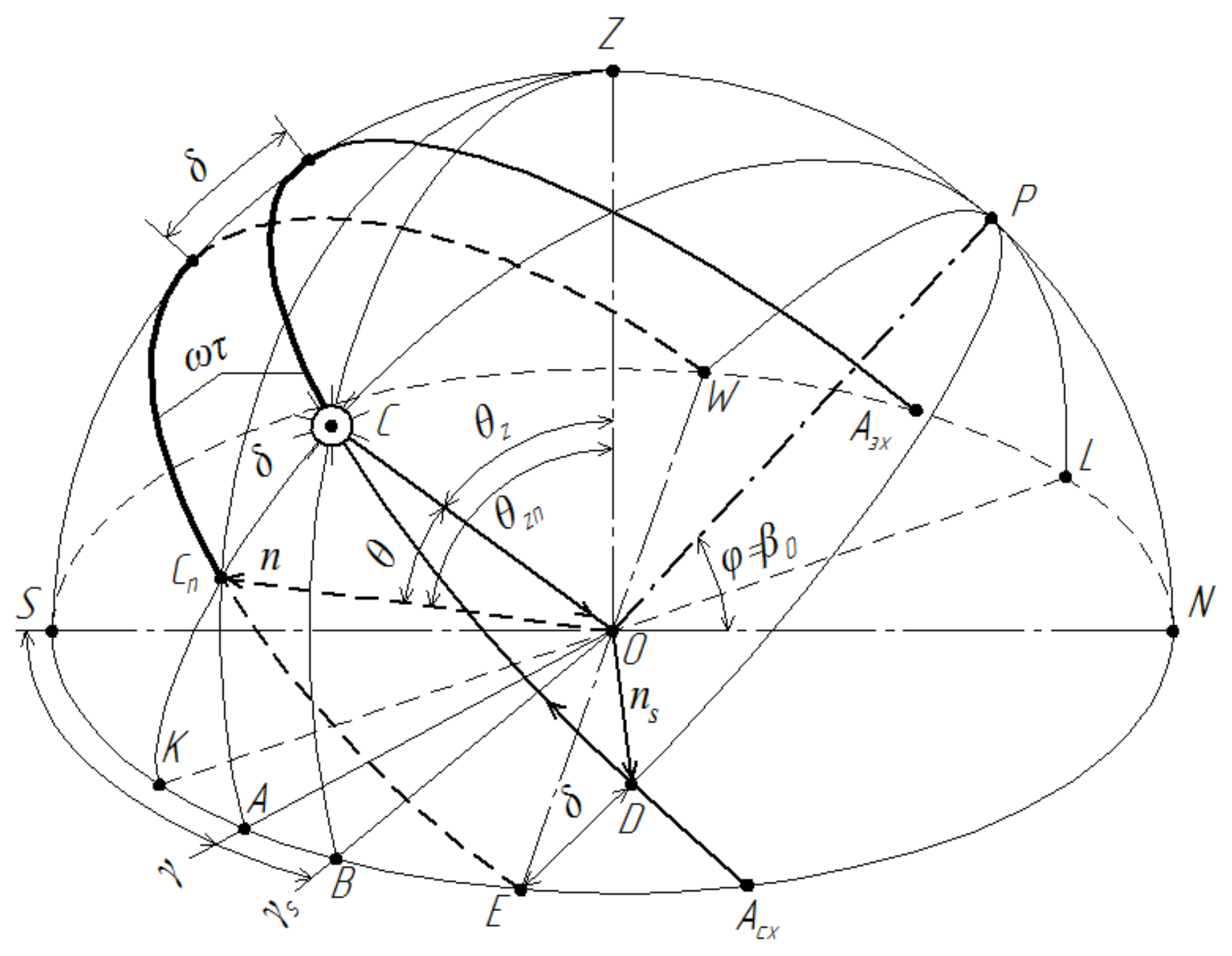
In other days of a year, pathways of the Sun and the normal of the tracking surface, combined with the rotating axis, do not coincide and conditions of irradiation are described by the general scheme, presented in Figure 14. The normal n of the tracking surface is demonstrated, not the very tracking surface. Daily path of the Sun along the skyline is marked by a continuous line of a standard width and the ends of the normal by a dash line, which coincides with the equinoctial line. Both trajectories stay in parallel planes, because their rotating centers are placed on a common polar axis OP.

In the equatorial system of sky coordinates, the synchronic tracking corresponds to the hourly angle ωτ, which is the same for the Sun and for the normal and is marked on the scheme by heavy parcels of both trajectories, limited by the arc of an equatorial vertical KC_nCP,, supported on the diameter KL. In the horizontal system of coordinates, different values of azimuth deflections of the normal γ and the Sun γ_s correspond to the same hour angles. The scheme demonstrates that they are limited by the points A and B of the intersection of the surface of the horizon with the surfaces of two horizontal verticals AC_nZ and BCZ.

Calculation of γ can also be performed for Equation (42) in case the zenith angle of the end of the normal is marked as θ_zn in a period of a year with a conventional deflection δ_n. Thus, under equality of hour angles of the Sun and the normal, the following equation is performed:

$$\mathit{s}\mathit{i}\mathit{n} \mathit{\omega }\mathit{\tau }\mathit{=}\frac{\mathit{s}\mathit{i}\mathit{n}{\mathit{\theta }}_{\mathit{z}\mathit{n}}\mathit{·}\mathit{s}\mathit{i}\mathit{n}\mathit{\gamma }}{\mathit{c}\mathit{o}\mathit{s}{\mathit{\delta }}_{\mathit{n}}}\mathit{=}\frac{\mathit{s}\mathit{i}\mathit{n}{\mathit{\theta }}_{\mathit{z}}\mathit{·}\mathit{s}\mathit{i}\mathit{n}{\mathit{\gamma }}_{\mathit{s}}}{\mathit{c}\mathit{o}\mathit{s} \mathit{\delta }}$$

(42)

hence,

$$\mathit{s}\mathit{i}\mathit{n} \mathit{\gamma }\mathit{=}\frac{\mathit{s}\mathit{i}\mathit{n}{\mathit{\theta }}_{\mathit{z}}\mathit{·}\mathit{s}\mathit{i}\mathit{n}{\mathit{\gamma }}_{\mathit{s}}\mathit{·}\mathit{c}\mathit{o}\mathit{s}{\mathit{\delta }}_{\mathit{n}}}{\mathit{s}\mathit{i}\mathit{n}{\mathit{\theta }}_{\mathit{z}\mathit{n}}\mathit{·}\mathbf{cos}\mathit{\delta }}$$

(43)

Current values of the azimuths of the Sun and tracking surface of orientation and energy efficiency are presented for the period of summer solstice in

Table 7. Orientation efficiency of the tracking surface while rotating around the polar axis, cosθ (own research).

τ, Hour	Summer Solstice						Spring Equinox		Winter Solstice
	γs	γ at β0 = φ	β0 = φ		β0 = φ − δ		β0 = φ		β0 = φ
			cosθ	E, W/m2	cosθ	E, W/m2	cosθ	E, W/m2	cosθ	E, W/m2
0	0	0	0.9174	969	1.0	1056	1.0	1026	0.9174	772
1	29.29	19.27	0.9174	967	1.0	1054	1.0	1017	0.9174	754
2	52.42	37.01	0.9174	952	1.0	1038	1.0	994	0.9174	688
3	69.60	52.55	0.9174	928	1.0	1012	1.0	943	0.9174	537
3.92	–	–		–	–	–	–	–	0.9174	328
4	83.12	66.14	0.9174	893	1.0	973	1.0	853	–	–
5	94.77	78.40	0.9174	835	1.0	910	1.0	634	–	–
6	105.6	90.00	0.9174	742	1.0	809	1.0	348	–	–
7	116.4	101.9	0.8861	552	1.0	623	–	–	–	–
8	128.1	114.2	0.7944	218	1.0	275	–	–	–	–
8.075	128.2	114.9	0.7852	183	1.0	233	–	–	–	–
H, W∙hours	–	–	–	13,907 91.2%	–	15,242 100%	–	11,282 100%	–	5267 90.1%

.

In case of combination of the tracking surface with the rotation axis, its normal $\overrightarrow{n}$ crosses the line of the horizon at the point E six hours after the full sun, while the Sun stays at the point D at the crossing of the sun’s trajectory with the arc of the equatorial vertical EPW. Since that moment and until the set (rise) of the Sun, a polar-rotating tracker is switched to passive tracking, with irradiation changes similar to the stationary, focused on the east (west) of the vertical surface, according to Equation (7) at:

$$\mathit{\gamma }\mathit{=}\mathit{\beta }\mathit{=}{\mathit{90}}^{\mathit{0}}$$

(44)

$$\mathbf{cos}\mathit{\theta }\mathit{=}\mathbf{sin}\mathit{\omega }\mathit{\tau }\mathit{·}\mathbf{cos}\mathit{\delta }$$

(45)

Duration of the passive regime on the day of a summer solstice can be measured by the evident equation:

$$\mathit{\tau }\mathit{=}{\mathit{\tau }}_{\mathit{c}\mathit{x}}\mathit{-}\mathit{6}$$

(46)

where 6 is hours, constituting 2.075 h for the latitude 50°. Hour values of the orientation and exposure efficiency are presented in Table 7 in the columns for the angle of initial (at full sun) inclination:

$${\mathit{\beta }}_{\mathit{0}}\mathit{=}\mathit{\phi }$$

(47)

A polar-rotating tracker also secures performance of seasonal optimization of the tracking surface efficiency by its deflection from the axis of rotation at the value of a current inclination:

-

in summer:

$${\mathit{\beta }}_{\mathit{0}}\mathit{=}\mathit{\phi }\mathit{-}\mathit{\delta }$$

(48)

-

in winter:

$${\mathit{\beta }}_{\mathit{0}}\mathit{=}\mathit{\phi }\mathit{-}\mathit{\delta }$$

(49)

Figure 15 demonstrates this as a combination of the trajectories of the normal $\overrightarrow{n}$ with direction to the Sun. Moreover, due to deflection towards the polar axis, the normal touches the line of the horizon, not six hours after the full sun, but earlier and simultaneously with the Sun. Thus, the one-axis polar-rotating tracker secures the same regime of irradiation as the double-axis one at the angle of deflection of the tracking surface from the axis of rotation, which is equal to the sun’s inclination.

The energy-saving double-axis tracker is constructively reasonable to be made in the structure of polar and horizontal axes. A drive unit of the polar axis can operate continuously in the mode of permanent angle speed 15 grad/hour, or be switched at equal time periods, e.g., hourly. In contrast, rotation around the horizontal axis is done much more seldom, with the average speed 2δ₀/183 = 46.9°/183 ≈ 0.26 grad/day. Correcting the inclination twice a month, the average deflection from the optimal direction to the Sun does not exceed 4°. In the majority of practical installations, such deflections are neglected, because they reduce irradiation of the tracking surface only by 0.23%. Hence, a double-axis tracker with the polar and horizontal axes can efficiently track the Sun according to the simplest synchronic algorithm of control. Thus, it can be easily composed by the simplest means of electronics without application of photosensitive sensors. In contrast, to operate non-sensor mirror concentrators, in which small deflections considerably influence the energy irradiation of the receivers, researchers employ more precise correlations between the angular dimensions, set by the model of the geocentric system of coordinates [38,39].

5. Conclusions

Issues of diurnal intensity distribution are based on the statistically averaged characteristics of the natural solar energy fluxes, which were considered in the description category for the actinometric optical mass index used to calculate the air transparency according to the models. For the standard model, the relative atmospheric mass is taken into account, the model does not depend on air pressure and density and, at the zenith of the beam deflection, the mass correlation is equal to the length correlation. In the Lambert model, the atmosphere is modeled as a spherical shell with a homogeneous density beyond the globe. However, for the geometric model according to Kasten-Jong, integral transparency of the real atmosphere is characterized by non-uniform distribution of pressure, temperature and humidity.

The optical thickness values are the starting parameters for calculating the practically important optical characteristics of the real atmosphere, i.e., visibility, turbidity, dust, etc. However, in both cases they depend on the optical mass of the air.

A novelty in the research is the use of the model in actinometry for air transparency. Values are quantified using parameters that depend on the optical mass along the beam path under clear sky conditions. In the atmosphere, the sun’s rays weaken due to the interaction of light with air molecules by two mechanisms, i.e., Rayleigh scattering and selective extinction of waves of a specific length of the solar spectrum by air molecules and their momentary fluctuations.

The use of the proprietary model enables a universal approach to the research, which showed that the values calculated according to Kasten were significantly underestimated because they were based on low-resolution spectral data.

In view of the above, the main conclusions are:

(1)

The final evaluation criteria for the performance of a solar tracking system can be obtained from complete data on both its components, i.e., orientation and exposure. Both are independent of weather conditions and are very precisely calculated from reconstructed values representing the basic laws of nature. Their defined time dependencies provide a specific specification of instantaneous (current) and total (integral) values within an hour of a day in a year.

(2)

The irradiation pattern and calculation methods can be easily adapted to the seasonal changes in the geographical coordinates of the area.

(3)

The tabular and graphical presentation of the results is convenient for quantifying the performance of rotary trackers, differing in their design and tracking algorithm.

(4)

The innovation of the work is based on the concept of a pole-rotating tracker, which ensures seasonal optimization of the tracking surface performance by deviating from the axis of rotation at the value of the current slope.