Reconstruction of Motion Images from Single Two-Dimensional Motion-Blurred Computed Tomographic Image of Aortic Valves Using In Silico Deep Learning: Proof of Concept

Abstract

The visualization of motion is important in the diagnosis and treatment of aortic valve disease. It is difficult to perform using computed tomography (CT) because of motion blur. Existing research focuses on suppressing or removing motion blur. The purpose of this study is to prove the feasibility of inferring motion images using motion information from a motion-blurred CT image. An in silico learning method is proposed, to infer 60 motion images from a two-dimensional (2D) motion-blurred CT image, to verify the concept. A dataset of motion-blurred CT images and motion images was generated using motion and CT simulators to train a deep neural network. The trained model was evaluated using two image similarity evaluation metrics, a structural similarity index measure (0.97 ± 0.01), and a peak signal-to-noise ratio (36.0 ± 1.3 dB), as well as three motion feature evaluation metrics, maximum opening distance error between endpoints (0.7 ± 0.6 mm), maximum-swept area velocity error between adjacent images (393.3 ± 423.3 mm²/s), and opening time error (5.5 ± 5.5 ms). According to the results, the trained model can successfully infer 60 motion images from a motion-blurred CT image. This study demonstrates the feasibility of inferring motion images from a motion-blurred CT image under simulated conditions.

1. Introduction

Aortic valve disease is the most common type of heart disease and a leading cause of cardiovascular morbidity and mortality [1]. It is a condition in which the valve between the left ventricle and the aorta does not open or close properly, thereby reducing or blocking blood flow and causing it to flow back. Aortic valve disease can be treated with two types of surgery: aortic valve repair surgery and aortic valve replacement surgery. Repair surgery is used to repair the aortic valve without removing the damaged valve, whereas replacement surgery is used to remove the damaged valve and replace it with an artificial aortic valve. Compared to replacement surgery, repair surgery usually preserves a large amount of original tissue and has a lower complication rate [2]. However, several difficulties remain in repair surgery. The feasibility of repair surgery primarily depends on the ability to reconstruct diseased valves. The success of repair surgeries depends on the degree of leaflet damage [3,4]. Additionally, universal application of repair surgeries has yet to be achieved, because of the lack of surgical expertise and experience [5]. To promote the application of repair surgeries, a more detailed understanding of anatomic structure and dynamic function of aortic valves is required, to accurately determine the degree of leaflet damage, appropriately select the surgical procedure, and make better surgical planning. Since the anatomic structure and dynamic function are closely related to motion, evaluating the motion of aortic valves is critical to achieving this goal.

Three main types of imaging techniques are available to assess aortic valves: echocardiography, cardiac magnetic resonance imaging (MRI), and cardiac computed tomography (CT). However, no matter which method is used, dynamic imaging of the aortic valve is still difficult because of its rapid movement [6]. Echocardiography is limited by its low spatial resolution and low frame rate (<20 fps) [7]. MRI and CT have a higher spatial resolution than echocardiography. Even with ECG-gated technology, MRI (<25 fps) and CT (<38 fps) [8] cannot meet the needs of dynamic imaging of aortic valves (>100 fps). Among these three imaging techniques, CT has emerged as a routinely used tool in the diagnosis of aortic valve diseases because of its high spatial resolution [9]. The temporal resolution of CT is limited by the scan time and angular range required for reconstruction. Therefore, when conducting cardiac CT, the rapid movements of aortic valves can cause motion blur. Due to the motion blur, the current CT diagnosis of aortic valves is limited to the analysis of the structure in the diastolic phase and does not use motion information. Motion blur remains a major challenge in cardiac CT diagnosis [10].

Many studies have been conducted to determine how to improve the quality of motion-blurred CT images. These techniques involve three main types: (1) physical methods, (2) image processing methods, and (3) machine learning methods. Physical methods are based on understanding the physics of motion blur and improving image quality using physical theory, such as decreasing the motion, increasing the number of X-rays, and ECG-gating [11]. These methods can slightly improve image quality, but they are limited by physical conditions and cannot handle fast motions. Image processing methods include image denoising and motion compensation [12]. Image denoising uses spatial or frequency domain filtering to remove noise, such as linear filters, nonlinear filters [13], total variation methods [14], and wavelet-based thresholding [15]. Motion compensation uses knowledge of motion to achieve image reconstruction [16], such as an anatomy-guided registration algorithm [17] and a second pass approach for aortic valve motion compensation [18]. Image processing methods perform better than physical methods, but they are not suitable for situations where the feature of motion blur is not obvious in the spatial or frequency domains or where the motion cannot be estimated in advance. Machine learning methods are data-driven approaches for removing or suppressing motion blur, such as using a neural style-transfer method to suppress artifacts [19] or using a motion vector prediction convolution neural network to compensate for motion blur [20]. These methods depend less on prior knowledge of motions and can reconstruct images more accurately. Although many methods have been proposed to improve the image quality of motion-blurred CT images, it is still difficult to analyze the rapid motion of aortic valves using the above-mentioned methods. These methods are limited, in that they only improve the image quality of a single blur image and do not provide motion images for motion analysis. To realize motion analysis with CT imaging, it is necessary to solve the ill-posed problem of inferring motion images from a single motion-blurred CT image.

Machine learning is famous for its ability to solve ill-posed problems. For example, a deep learning neural network (DNN) in optical imaging has successfully extracted a video sequence comprising seven frames from a single motion-blurred image [21]. However, there is currently no relevant research on inferring motion images from motion blur in CT imaging. It is considered that the projection data for reconstructing a CT cross-section image corresponds to the valve motion information when each projection datum is obtained. Our central hypothesis is that information about dynamic valve motion, including opening time and maximum opening distance of the valve leaflets, can be retrieved from a single motion-blurred CT image. Since the relationship between the motion information embedded in the projection data and the resultant motion-blurred CT image is complex, we assume that a DNN can relate the motion-blurred CT image information to the corresponding time series of the valve motion information.

This study aims to prove that motion images can be inferred from motion blur in CT images of aortic valves. In this case, motion blur is no longer considered an undesirable phenomenon to be removed, but a valuable source of information on the dynamics of aortic valves. The in silico learning method [22] was used to prove the proposed concept, because it allows for discovering and demonstrating new concepts with a combination of the in silico dataset and deep learning. In our hypothesis, the motion information in motion-blurred CT images’ is critical for achieving the goal. Therefore, to test the hypothesis, we have employed simple numerical simulation experiments with a 2D CT simulator and valve models, where a CT image was reconstructed with multiple projection data captured at different instant motion images. When a 2D CT scan is performed from the direction perpendicular to the aortic annulus, the motion of aortic valves can be approximated to 2D motion. Furthermore, to show the ability of motion blur in inferring motion images, only the motion blur in the CT images was considered in the simulation. With these simplifications, we proposed an in silico learning scheme that combined a simulation dataset and deep learning to infer 60 motion images from a single motion-blurred CT image to prove the proposed concept. To the best of our knowledge, this is the first time that this problem has been proposed and studied in the CT imaging field.

2. Methods

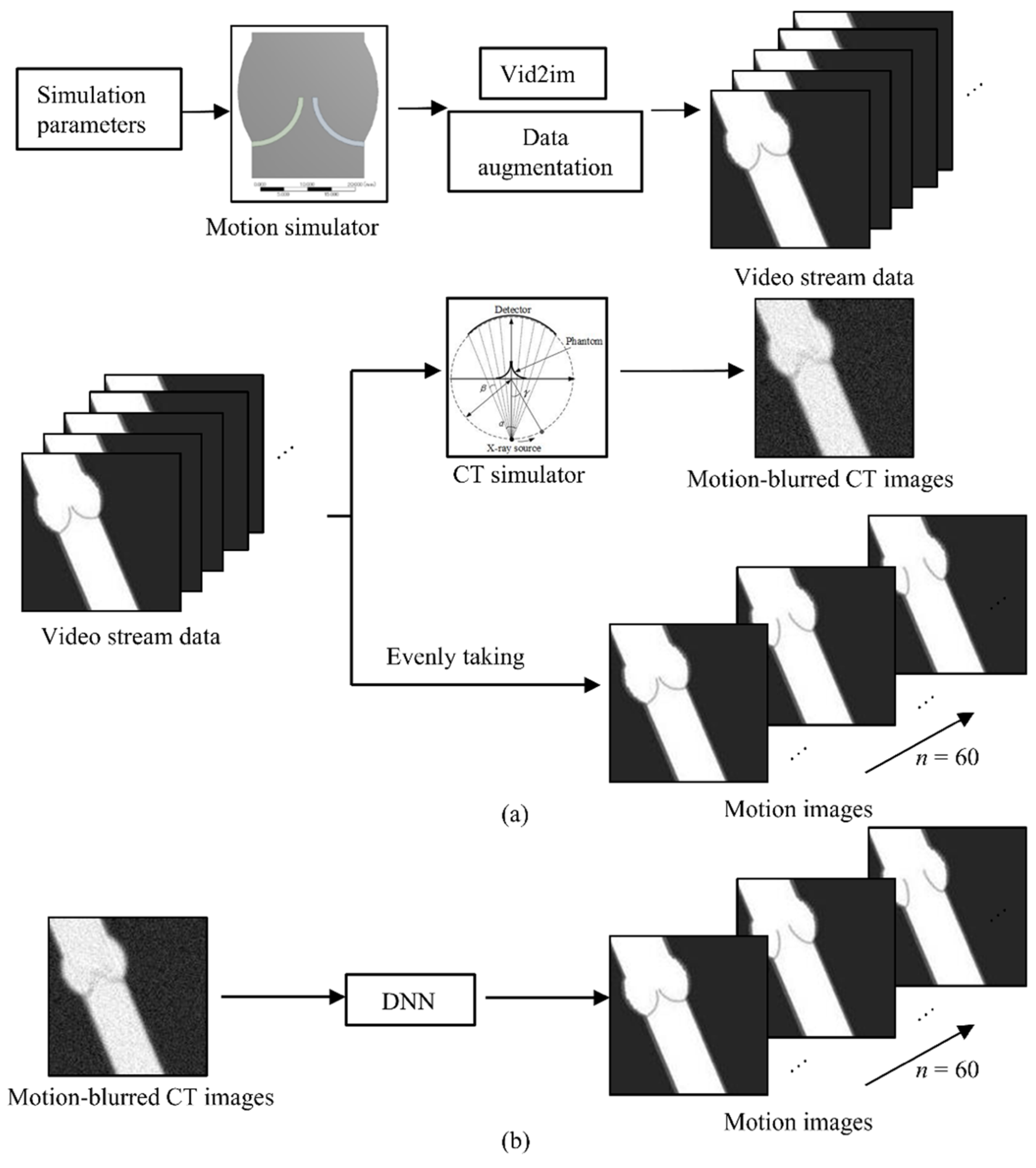
To demonstrate the concept that motion information can be obtained from motion blur in the CT imaging field, we proposed an in silico learning scheme to infer 60 motion images from a single motion-blurred CT image. The overview of the proposed in silico learning scheme is shown in Figure 1. The proposed method consists of two parts: (a) data generation process and (b) DNN training process. The dataset generation process is shown in Figure 1a. First, various simulation parameters were input into the motion simulator to generate different motion videos. The generated motions differed in motion features, such as velocity and maximum opening distance of aortic valves by varying the geometric parameters and material properties of aortic valves. In the Vid2im module, we converted motion videos to images, painted background tissues to these images, assigned grayscale values to each component, and finally converted these images to a specified spatial resolution to make video stream data. After data augmentation such as translation and rotation, the number of the video stream data was increased. Finally, video stream data was input into the CT simulator, which simulated the projection process and reconstruction process. The CT simulator generated motion-blurred CT images from the video stream data. Then, 60 motion images to be inferred were selected at equal time intervals from video stream data used in CT imaging. A dataset, containing pairs of motion-blurred CT and motion images, was generated in this manner. The DNN training process is shown in Figure 1b. A DNN was trained on the generated dataset. The input and output of the DNN are a single motion-blurred CT image and 60 motion images, respectively. The details of the components are described below.

2.1. Data Generation Process

To generate a dataset with a reasonable movement of aortic valves in the motion images and rational motion blur patterns in the motion-blurred CT images, 2D motion and 2D CT simulators were used. Since the movement of aortic valves is a two-way fluid structure interaction theory (2-way FSI) problem, the motion simulator was designed on the ANSYS (2021R1, ANSYS) platform based on 2-way FSI [23]. In 2-way FSI, blood flow is affected by valve displacement, and the valve is affected by the force generated by blood flow. 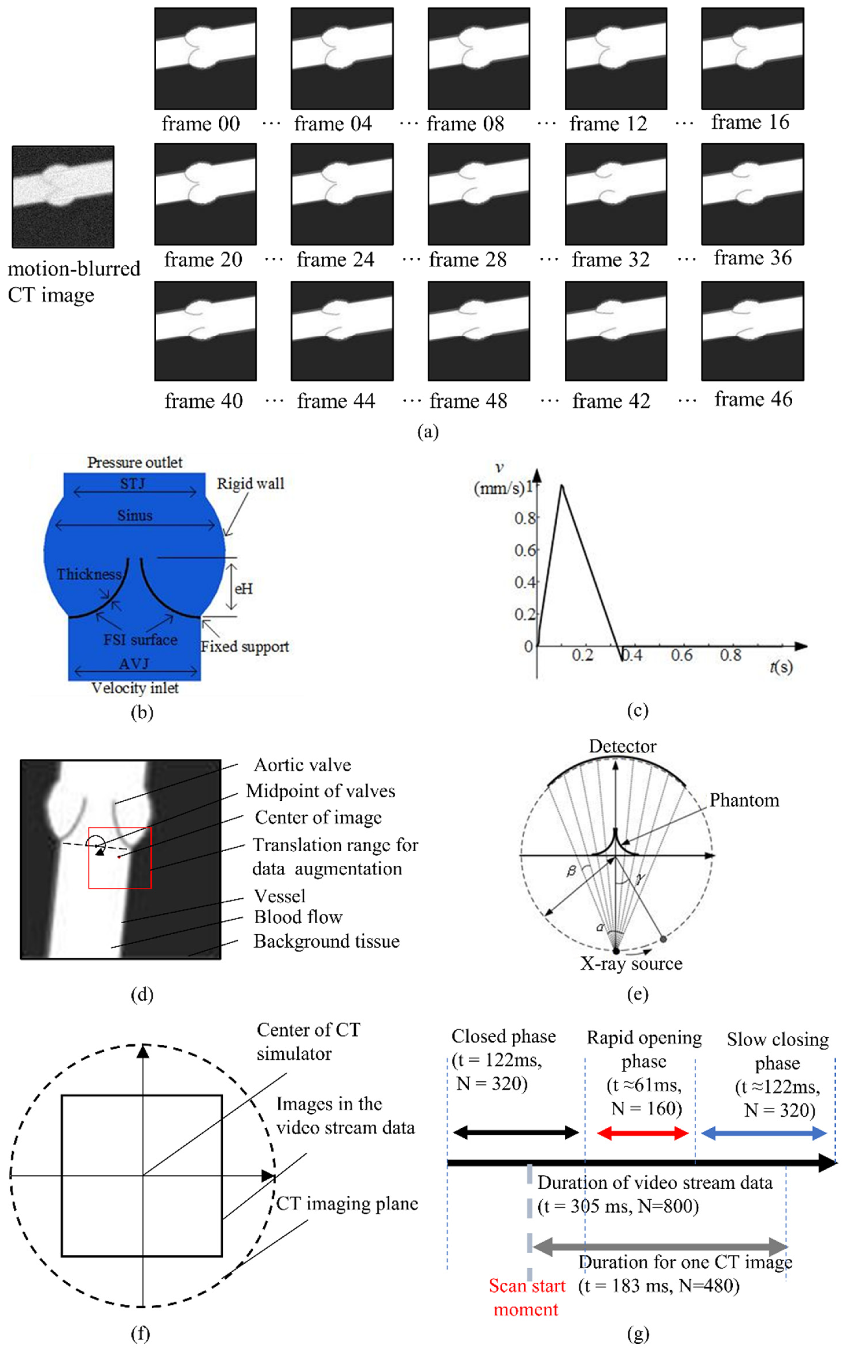The CT simulator was designed based on a ray-driven simulation method [24] on the MATLAB (R2022a, MathWorks) platform. A sample of the data is shown in Figure 2a. The detailed data generation process is presented below.

2.1.1. Motion Simulator

To generate a reasonable movement of aortic valves, a 2D motion simulator was designed on ANSYS Workbench platform based on 2-way FSI theory. ANSYS FLUENT and ANSYS MECHANICAL APDL were used to solve the fluid and structure fields, respectively. These two fields were coupled using the system coupling module. Although the motion simulator cannot perfectly simulate the real physical process, it can reproduce the complex motion variation depending on FSI.

The geometries of the numerical model were developed using the geometry study of aortic valves [25,26]. The geometry of aortic valves is shown in Figure 2b, and the geometric parameters are shown in

Table 1. Geometric parameters of aortic valves (mean ± std).

Parameters	Size (mm)
Thickness	0.42 ± 0.12
eH (Effective height)	9.5 ± 1.4
Ad (Aorto-ventricular diameter)	21.0 ± 2.8
Sd (Sinus Valsalva diameter)	28.5 ± 3.5
STJ (Sinotubular junction)	25.0 ± 3.7

. These geometric parameters were sampled according to the normal distribution with the known mean and standard deviation of each parameter in Table 1.

In the structure field, the material properties of aortic valves were defined. For simplicity, a linear elastic material model was used. The values of these parameters were selected using FSI studies in this area. The detailed parameters are shown in

Table 2. Material properties of aortic valves.

Parameters	Range for Random Selection
Density (kg/m3)	1000, 1020, 1056, 1060, 1100, 1250
Young’s modulus (Mpa)	2–8
Poisson ratio	0.49, 0.4, 0.3, 0.45

. These material parameters were sampled according to the random distribution, with the known range of each parameter, in Table 2.

In the fluid field, the parameters of blood flow were defined. For simplicity, the blood flow was assumed to be incompressible Newtonian with constant blood density of 1060 kg/m³, constant viscosity of 0.0035 J/s. For turbulence modeling, the k-ε model was used [27]. The inlet was defined as the velocity inlet. Based on the measurement of Doppler [28], a patient specified inlet velocity was used (Figure 2c).

The main causes of aortic valve diseases are changes in geometry and material properties [29]. By varying the geometric parameters and material properties, 80 motion videos with different velocities and deformations were generated. With the generated videos, we extracted image frame by frame from motion videos to generate video stream data in the Vid2im module. The images in the video stream data are grayscale images with a size of 512 × 512 and a spatial resolution of 0.5 mm/pixel. An image in the video stream data is shown in Figure 2d. Background tissue was painted in the video stream data in the Vid2im module to make the data more realistic. The pixel values of each component are determined using the CT value (

Table 3. CT values and normalized pixel value of each component in the motion image.

Components	CT Value (HU)	Pixel Values
Vessels and aortic valve	118	92
Blood flow	330	255
Background tissue	52	38

). The proportion of each component was used to determine the pixels of the contact area among the aortic valve, blood, and background tissue. The midpoint of the aortic valves was defined as the midpoint of the aortic annulus (Figure 2d). In the data augmentation process, we translated the midpoint of aortic valves in the range of −5–5 mm from the center of the images and rotated the aortic valve in the range of 0°–360° around the midpoint of aortic valves, to augment the number of the video stream data. Finally, 8000 video stream data were generated from 80 motion videos, and each motion video corresponds to 100 video stream data. The duration of the video stream data is 305 ms (Figure 2g). Each video stream data contains 320 images of the closed phase, 160 images of the rapid opening phase, and 320 images of the slow closing phase. Here, we did not include motions of the rapid closing phase [30] and only used part of the motion to demonstrate the proposed concept that motion images of aortic valves can be inferred from motion-blurred CT images.

2.1.2. CT Simulator

A 2D equiangular fan-beam CT simulator was used to generate rational motion blur patterns in the motion-blurred CT images. It is a complex physical process, in which X-rays from the source pass through an object and are collected by the detector. In this study, we only focused on the motion blur caused by the motion of the aortic valves. Therefore, the complex physical process can be well-approximated by taking collections of line integrals and combining them in appropriate ways [31]. The geometry of the 2D equiangular fan-beam CT is shown in Figure 2e. The X-ray source was rotated from −90° of the imaging plane. The parameters of the CT simulator are shown in

Table 4. Parameters of the fan-beam CT simulator.

Parameters	Value
Fan angle	60°
Rotation angle increment	0.5°
Fan-beam spacing	0.25°
Time required for one image	183 ms
Spatial resolution	0.5 mm/pixel

.

We used a ray-driven CT simulation method. The ray-driven method connects a line from the focal point through the image to the center of the detector cell of interest of the X-ray. CT values along the X-ray were calculated by interpolation of adjacent pixels. In the projection process of the CT simulator, the projection data is given by the following:

$$p\left(r\right)=\int \mu \left(x,y\right)ds$$

(1)

where $\mu \left(x,y\right)$ is the attenuation coefficient at the point (x, y), s is the ray from the source to the detector, and the projection data $p\left(r\right)$ is the line integral along with the X-ray. In the reconstruction process, the filtered back projection (FBP) [32] and half scan reconstruction [33] algorithms were used to reconstruct motion-blurred CT images from projection data. The back-projection data is given by the following:

$$b\left(x,y\right)=\int p\left(s,\theta \right)d\theta$$

(2)

where $b\left(x,y\right)$ is the back-projection data at the point (x, y), θ is the rotation angle of X-rays.

A single motion-blurred CT image requires about 183 ms of video stream data (Figure 2g). Considering that the CT scan cannot start at the precise moment the aortic valve starts to open in the real world, we randomly selected the scan start moment to generate motion-blurred CT images. The time range for random scan start is during the closed phase of aortic valves, because motion images in the rapid opening phase are relatively important to understanding the dynamics of aortic valves. Images from the video stream data were set in the CT imaging plane in the simulator, and the center of images in the video stream data was kept the same as the center of the CT simulator (Figure 2f). After inputting the video stream data to the CT simulator, we can acquire motion-blurred CT images. Additionally, motion images were evenly taken from the video stream data used in CT imaging. Finally, we selected a 128 × 128 region around the center of the images to make the dataset. In this way, a dataset (N = 8000) containing motion-blurred CT and their corresponding 60 motion images was generated. The dataset was further divided into a training dataset (N = 6400), validation dataset (N = 800), and test dataset (N = 800).

2.2. DNN Training Process

2.2.1. Network Architecture

As explained, we assume that DNN can relate the motion-blurred CT image information to the corresponding time series of the valve motion information. In fact, several different architectures were used to confirm the feasibility of this idea. These data show that DNN can represent the relationship between a motion-blurred CT image to the corresponding valve motion information embedded in the projection data used (the comparison study of 4 different models can be seen in Supplementary Materials). We used the proposed architecture in the paper because of its better performance. 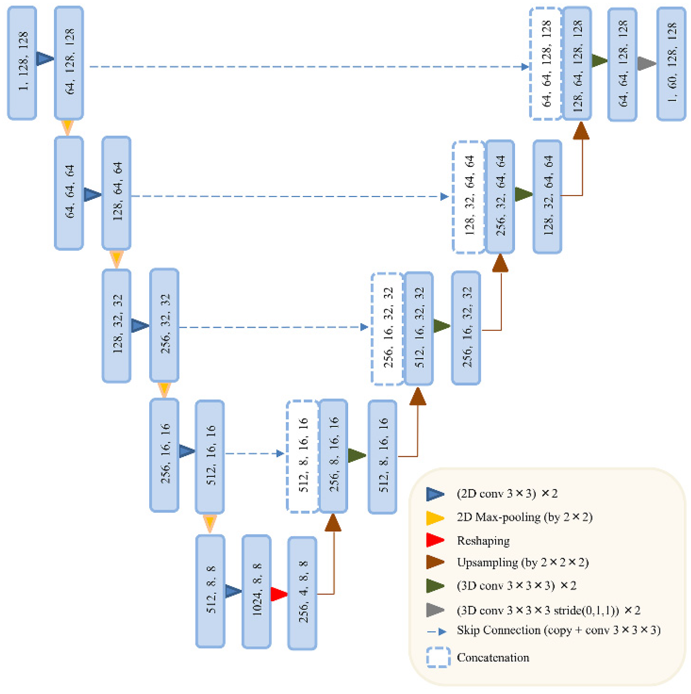Figure 3 shows the detailed network architecture of our proposed model. The model was built on a 2D U-Net [34]. It is a powerful technique to locate objects or boundaries in images on a per-pixel level and encode the input image into feature representations at multiple different levels. Moreover, it has advantages of its concise architecture design, fast convergence in training, and high representation power. Although it enables to fully extract the features of motion-blurred CT images, 2D convolution limits its ability to extract temporal features. Several modifications were made to meet the requirements. Although the 2D U-Net was designed for segmentation problems, we can use it for our problem by changing the activation function to a sigmoid function and employing mean square error (MSE) loss function. Additionally, we modified the decoder of the 2D U-Net with the decoder of the three-dimensional (3D) U-Net [35]. This 5-layer 3D decoder can learn temporal features from spatial features and enable the information changes between temporal and spatial features. Moreover, a special skip connection module was used to enable the information changes between the 2D encoder and 3D decoder. In the skip connection module, 2D features extracted in the encoder part were copied to the size of the 3D features in the 3D decoder. Then, a 3D convolution operation was performed to select useful features in each dimension. Based on these changes, the proposed model can infer 60 motion images from one motion-blurred CT image. The input to the network is one motion-blurred CT image with size 1 × 128 × 128 (channel × width × height), whereas the output of the network is 60 motion images with size 1 × 60 × 128 × 128 (channel × depth × width × height), in which the time series was treated as the depth dimension.

2.2.2. Loss Function

The MSE is the most commonly used regression loss function, which is defined as the following:

$$\mathrm{MSE}=\frac{1}{mn}{{\displaystyle \sum }}_{i=1}^m{{\displaystyle \sum }}_{j=1}^n{\left(Y_{ij}-Y_{ij}^p\right)}^2$$

(3)

where m is the number of training data, n is the number of motion images for each training data (n is equal to 60 in this study), $Y_{ij}$ is the ground truth motion image, and $Y_{ij}^p$ is the predicted motion image.

2.2.3. Implementation Detail

The network was trained in Pytorch using three GTX 2080 Ti GPUs (NVIDIA). The batch size is six. We use Adam optimizer for its good convergence and fast running time, with a learning rate as 10⁻⁴; the hyperparameters β₁ and β₂ were 0.9 and 0.999, respectively, and the weight decay was 10⁻⁶. The learning rate was determined by a trial-and-error method, and the value that demonstrated the best loss without compromising the speed of training is selected. We tried exponential values: 10⁻², 10⁻³, and 10⁻⁴. The final validation losses are 5.6 × 10⁻⁴, 3.2 × 10⁻⁴, and 2.3 × 10⁻⁴, respectively. The learning rate 10⁻⁴ was determined because of the lowest validation loss.

2.3. Evaluation Metric

To better evaluate the performance of our model, we used not only image similarity evaluation metrics but also motion feature evaluation metrics. In terms of image similarity metrics, the structural similarity index measure (SSIM) and peak signal-to-noise ratio (PSNR) were used. In terms of motion feature evaluation metrics, the maximum opening distance error between endpoints (MDE), the maximum-swept area velocity error between adjacent images (MVE), and the opening time error (OTE) was introduced. MDE and MVE can evaluate the intensity of the motion, whereas OTE can evaluate the temporal order of the motion.

2.3.1. Image Similarity Evaluation Metrics

The SSIM metric is a perception-based metric for measuring the similarity between two images that considers image degradation as a perceived change in structural information and incorporates important perceptual phenomena, such as luminance and contrast. SSIM is defined as the following:

$$\mathrm{SSIM}\left(x,y\right)=\frac{\left(2{\mu }_x{\mu }_y+c_1\right)\left(2{\sigma }_{xy}+c_2\right)}{\left({\mu }_x^2+{\mu }_y^2+c_1\right)\left({\sigma }_x^2+{\sigma }_y^2+c_2\right)}$$

(4)

where ${\mu }_x, {\mu }_y$ is the mean of x, y, respectively; ${\sigma }_x^2, {\sigma }_y^2$ is the variance of x, y, respectively; ${\sigma }_{xy}$ is the covariance of x and y; and c₁, c₂ are two variables to stabilize the division with weak denominator.

The PSNR is the most widely used objective image quality metrics for evaluating the similarity between two images. The PSNR is defined as the following:

$$\mathrm{PSNR}=10·{\log }_{10}\left(\frac{MA{X}_I^2}{\mathrm{PSNR}}\right)$$

(5)

where $MA{X}_I^2$ is the maximum possible pixel value of images.

2.3.2. Motion Feature Evaluation Metrics

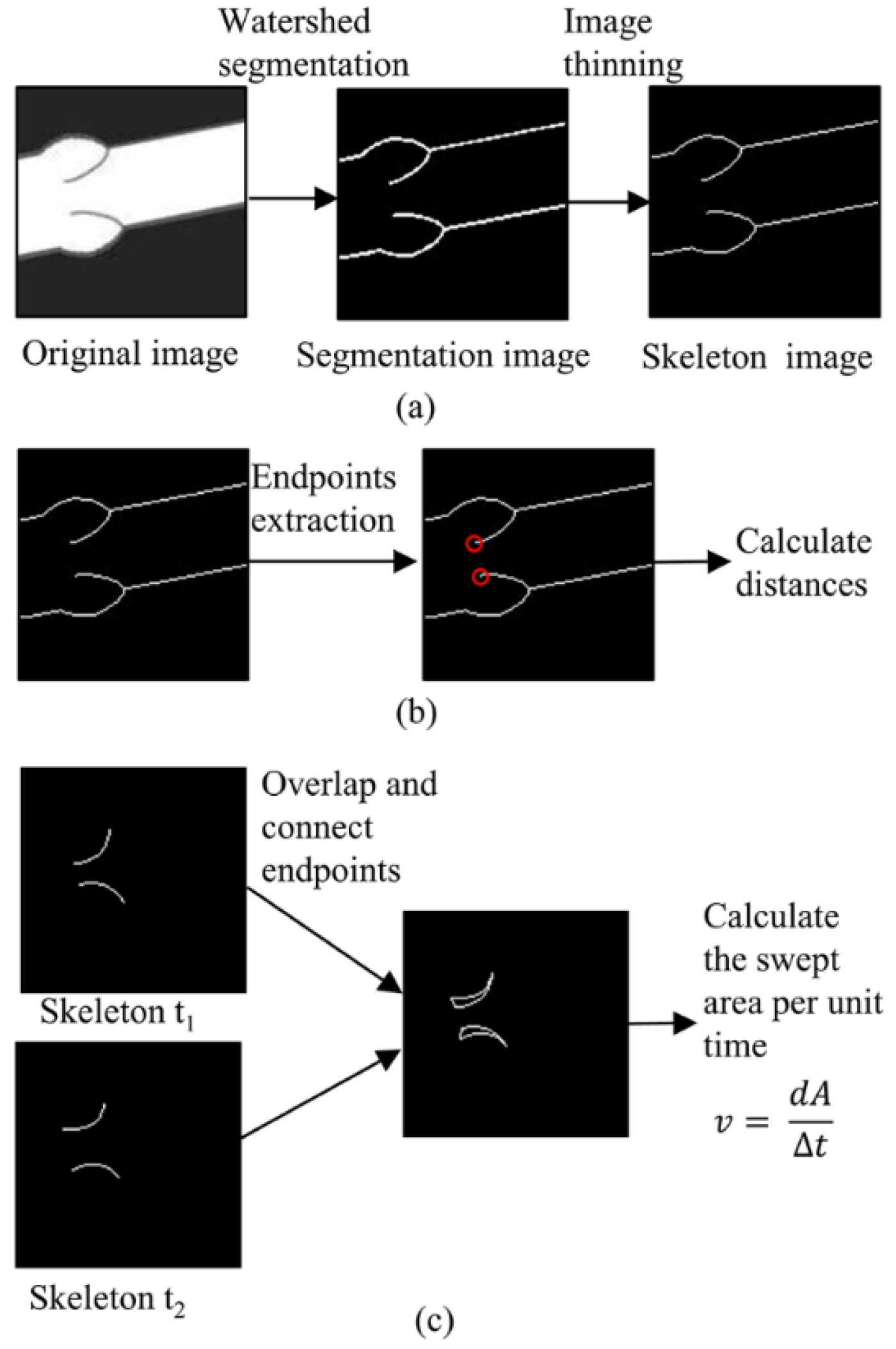
To evaluate the MDE, MVE, and OTE of the motion, we used skeleton images to avoid the influence of the aortic valve thickness on calculating opening distance and swept area velocity. The original image is segmented based on the marker-based segmentation method [36], and the segmentation image is skeletonized using the image thinning method [37] (Figure 4a). We manually extracted the skeleton images for the failed cases.

The MDE is used to evaluate the maximum opening distance of endpoints between ground truth motion and predicted motion images. The opening distance between endpoints was calculated using the coordinates from endpoints extraction (Figure 4b). Then, the maximum opening distance is determined from the distances of all motion images. The MDE is defined as the following:

$${\epsilon }_{\mathrm{MDE}}=\frac{1}{N}{{\displaystyle \sum }}_N\left|d_{o\_pre}-d_{o\_g}\right|$$

(6)

where $d_{o\_pre}$ is the maximum opening distance of the endpoints of the predicted motion images, $d_{o\_g}$ is the maximum opening distance of the endpoints of ground truth motion images.

The MVE is used to evaluate the area swept velocity by the aortic valve between ground truth and prediction. The swept area velocity between adjacent images is defined as the area swept out by the skeleton of the aortic valve per unit time (Figure 4c)

$$v_A=\frac{dA}{dt}$$

(7)

where dA is the area swept out by the skeleton of aortic valve during the time of dt. The MVE is defined as the following:

$${\epsilon }_{\mathrm{MVE}}=\frac{1}{N}{{\displaystyle \sum }}_N\left|v_{m\_pre}-v_{m\_g}\right|$$

(8)

where $v_{m\_pre}$ is the maximum-swept area velocity of predicted motion images, $v_{m\_g}$ is the maximum-swept area velocity of ground truth motion images.

The OTE is used to evaluate the opening time between the ground truth and predicted motion images. The aortic valve opening time was defined as the point at which the endpoint distance was 1 mm larger than the initial state. Since the spatial resolution of the CT image is 0.5 mm/pixel, 1 mm is an approximate distance change value when the endpoints of aortic valves move one pixel away from the initial location. The OTE is defined as the following:

$${\epsilon }_{\mathrm{OTE}}=\frac{1}{N}{{\displaystyle \sum }}_N\left|t_{o\_pre}-t_{o\_g}\right|$$

(9)

where N is the number of test dataset, N = 800. $t_{o\_pre}$ is the opening time of the predicted motion images, and $t_{o\_g}$ is the opening time of the ground truth motion images.

3. Results

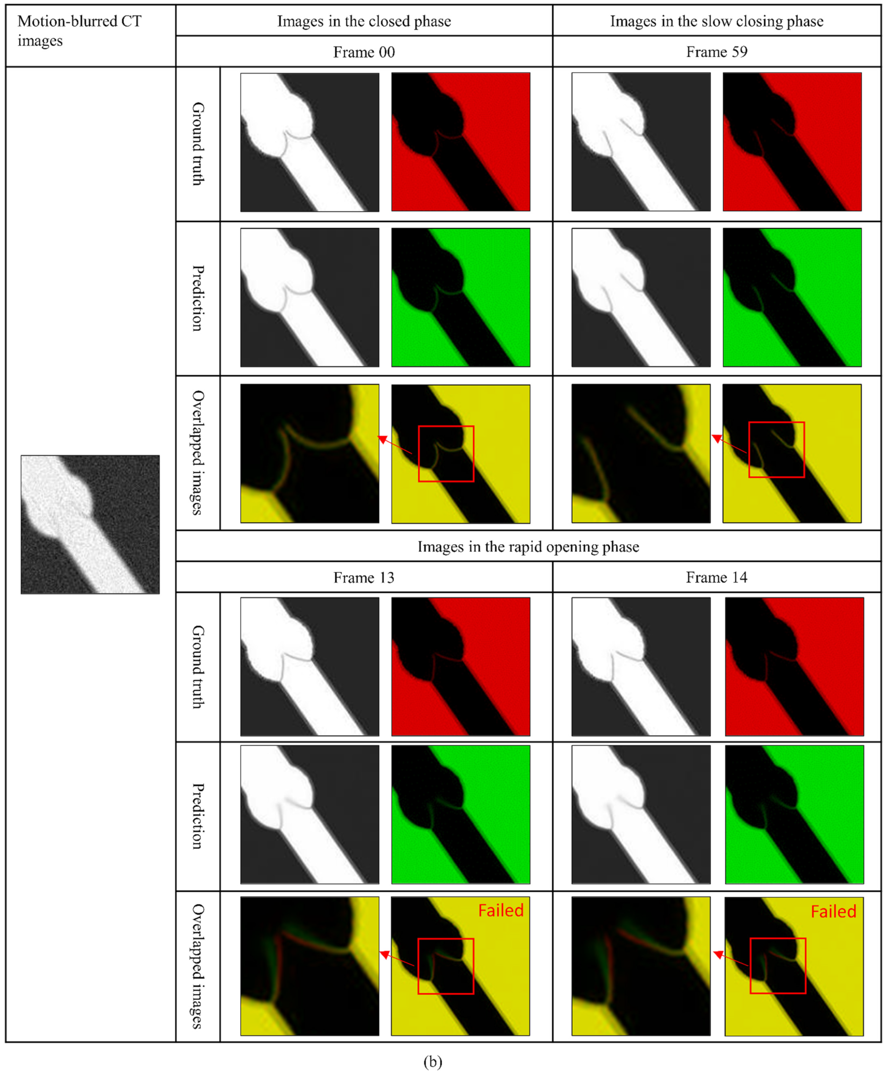
To evaluate the trained model, a test dataset containing 800 pairs of motion-blurred CT images and their corresponding 60 motion images was used. It was generated from eight different motion videos that were excluded from the training dataset. Two examples of the performance of the trained model are shown in Figure 5. We only selected several images as the representative of each phase to qualitatively analyze the performance of our model. Overlapped images were used to demonstrate the structural similarity between the prediction and ground truth. They were produced by overlapping color images that were converted from the ground truth and predicted images. In the overlapped images, correctly predicted pixels will turn yellow or remain black, whereas mispredicted pixels will remain green and red. A typical example with good performance is shown in Figure 5a. There are few green and red pixels in the overlapped images (Figure 5a), indicating that the structures of predicted images are close to the ground truth images. A typical example with bad performance is shown in Figure 5b. Predicted images in the closed phase and predicted images in the slow closing phase are close to the ground truth images (Figure 5b). However, predicted images during the rapid opening phase differ from the ground truth images. There are significant branches with green and red pixels in the overlapped images of these images. To further learn the distribution of correct and failed predictions, 50 pairs of motion-blurred CT images and their corresponding 60 motion images were randomly selected from the test dataset. Then, we checked overlapped images. Correctly predicted motion images were treated as correct predictions, while mispredicted motion images were treated as failed predictions (

Table 5. The distribution of correct predictions and failed predictions.

Probability	Images in the Closed Phase (N = 989)	Images in the Rapid Opening Phase (N = 1000)	Images in the Slow Closing Phase (N = 1011)
Correct prediction	92.3%	68.6%	83.3%
Failed prediction	7.7%	31.4%	16.7%

). A considerable performance drop can be seen in the rapid opening phase.

To evaluate the trained model quantitatively, we used two image similarity evaluation metrics and three motion features evaluation metrics. The details are presented below.

3.1. Results of Standard Image Quality Metrics

Table 6. Evaluation results of SSIM and PSNR (N: the number of images, mean ± std).

Images in Different Phases	SSIM	PSNR (dB)
All images (N = 48,000)	0.97 ± 0.01	36.0 ± 1.3
Images in the closed phase (N = 15,983)	0.98 ± 0.01	36.4 ± 1.1
Images in the rapid opening phase (N = 16,000)	0.97 ± 0.01	35.5 ± 1.5
Images in the slow closing phase (N = 16,017)	0.97 ± 0.01	35.9 ± 1.1

shows the SSIM and PSNR of the trained model. There are 48,000 motion images in total. Additionally, we recorded the number of images in the different phases in advance. The number of images in the closed phase is 15,983, the number of images in the rapid opening phase is 16,000, and the number of images in the slow closing phase is 16,017. We evaluated the accuracy of all images, images in the closed phase, images in the rapid opening phase, and images in the slow closing phase of aortic valves (Table 6). The SSIM and PSNR of all images and images of different phases are close, as shown in the table. Moreover, images in the closed phase have the highest accuracy, images in the slow closing phase have the second-highest accuracy, and images in the rapid opening phase have the worst accuracy.

3.2. Results of Motion Feature Evaluation Metrics

Table 7. Evaluation results of MDE, MVE, and OTE (N: the number of motion images, mean ± std).

Evaluation Metrics	Values
MDE (N = 800)	0.7 ± 0.6 (mm)
MVE (N = 800)	393.3 ± 423.3 (mm2/s)
OTE (N = 800)	5.5 ± 5.5 (ms)

shows the results of motion feature metrics: MDE, MVE, and OTE. The geometric parameters and material properties of aortic valves with eight different motions in the test dataset are shown in

Table 8. Geometric parameters of aortic valves with eight motions in the test dataset.

Motion No.	Thickness (mm)	eH (mm)	Ad (mm)	STJ (mm)	Sd (mm)
1	0.39	8.4	17.7	20.6	26.7
2	0.54	9.5	20.2	24.6	29.7
3	0.24	9.2	19.4	26.3	29.6
4	0.54	9.8	21.3	25.1	30.3
5	0.39	10.1	21.4	24.5	29.8
6	0.60	9.8	21.2	24.6	29.9
7	0.46	8.6	18.7	19.4	25.9
8	0.35	8.7	18.4	25.5	29.9

and

Table 9. Material properties of aortic valves with eight motions in test dataset.

Motion No.	Density (kg/m3)	Young’s Modulus (Mpa)	Poisson Ratio
1	1250	4.0	0.40
2	1100	3.8	0.45
3	1020	5.4	0.49
4	1250	6.8	0.45
5	1000	4.4	0.49
6	1000	6.1	0.49
7	1000	7.5	0.49
8	1060	2.7	0.45

, respectively. The maximum opening distance and maximum-swept area velocity of the aortic valves with eight different motions are shown in

Table 10. Maximum opening distance and maximum-swept area velocity of aortic valves with eight motions (dmax: maximum opening distance of ground truth, dmax_p: maximum opening distance of prediction, Vmax: maximum-swept area velocity of ground truth, Vmax_p: maximum-swept area velocity of prediction) (mean ± std).

Motion No.	dmax (mm)	dmax_p (mm)	Vmax (103 mm2/s)	Vmax_p (103 mm2/s)
1	10.9	10.6 ± 0.6	1.6	1.4 ± 0.3
2	12.0	11.7 ± 0.5	1.8	1.7 ± 0.2
3	15.2	13.9 ± 0.8	2.4	1.9 ± 0.4
4	12.2	11.8 ± 0.5	1.8	1.8 ± 0.2
5	13.9	13.5 ± 0.6	2.4	2.1 ± 0.4
6	11.8	11.3 ± 0.7	1.7	1.7 ± 0.3
7	10.0	9.6 ± 0.7	1.3	1.2 ± 0.3
8	13.1	12.6 ± 0.7	2.1	1.7 ± 0.3

. Since the CT scan starts moments differ, the maximum opening distance and maximum-swept area velocity differ slightly in each pair of motion images of a single motion. For simplicity, we used the mean maximum opening distance and the mean maximum-swept area velocity as the ground truth.

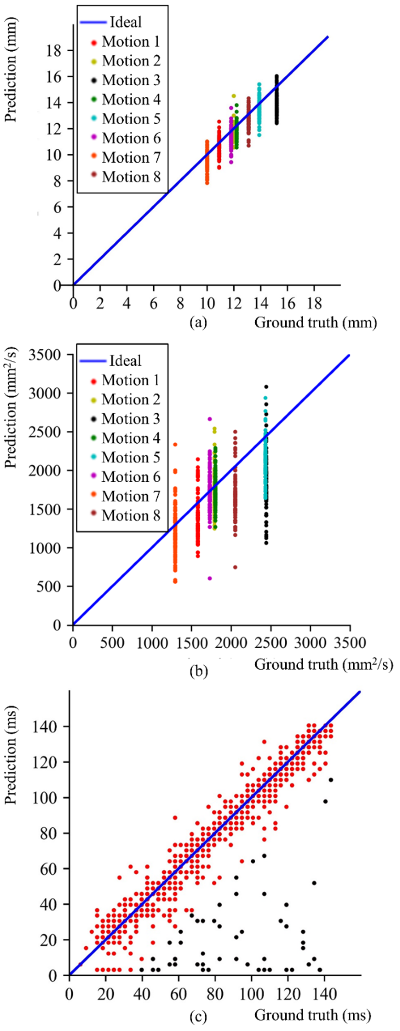
To visualize the performance of our trained model, the data distribution map of maximum opening distance, maximum-swept area velocity, and opening time are shown. Ideally, these points should be distributed on the blue line. The data distribution of maximum opening distance is shown in Figure 6a. The data distribution of maximum-swept area velocity is shown in Figure 6b. The data distribution of opening time is shown in Figure 6c. The black points are outliers that differ significantly from the ground truth, and they account for approximately 6.6% of the total.

4. Discussion

In this study, the proposed concept of inferring aortic valve motion images from a single motion-blurred CT image was demonstrated using in silico learning under certain conditions. After training with the simulated dataset, the performance of the trained model was evaluated using two image similarity evaluation metrics and three motion feature evaluation metrics. The results of two image similarity evaluation metrics (SSIM, PSNR) are shown in Table 6. By analyzing and comparing these results, we found that the trained model can learn motion images from motion blur. The accuracy of different phases was different; additionally, a correlation between velocity and accuracy was observed: the higher the velocity, the lower the accuracy. We further explored the velocity limitation of the trained model, which works under the condition of the swept area velocity below 1400 mm²/s. The results of three special evaluation metrics (MDE, MVE, and OTE) are shown in Table 7. After analyzing the results of these metrics, we found that the trained model can infer opening time with a high accuracy and also had some ability in predicting maximum opening distance and maximum-swept area velocity. Furthermore, these motion features may be used to roughly determine the material properties of aortic valves.

Despite the velocity limitation, this study shows that the trained DNN has learned the motion images from a single motion-blurred CT image of aortic valves. The main difference between the proposed and traditional methods is the way to deal with motion blur. In the proposed method, the motion information hidden in the motion blur is learned via DNN to infer motion images, whereas traditional methods primarily use the spatial or transform domain distribution of the motion blur to suppress or remove motion blur. For example, a wavelet-based thresholding method [16] removed noise by finding some thresholds in the wavelet transform domain. In some motion compensation methods, additional information is used, but this information is only used to separate targets from motion blur, while the motion information in blur is not used. For example, an anatomy-guided registration algorithm [17] used anatomy structure to compensate for regions of interest and remove extra noise. This difference in method leads to differences in results. Our method can reconstruct the entire time series representing the valve motion from a single motion-blurred CT image. However, the conventional method recovers an image without temporal information from a single motion-blurred CT image. Motion images can provide far more information than a single image, such as motion features. Moreover, the amount of information in results between the proposed and traditional methods is different, indicating that the proposed method is considerably different from the traditional methods.

4.1. Interpretation of Image Similarity Evaluation Metrics

To understand the improvement in the image quality between the motion-blurred CT and predicted images, we compared the SSIM and PSNR of motion-blurred CT and predicted images, respectively. The SSIM and PSNR differences between motion-blurred CT images and ground truth motion images are 0.41 ± 0.02 and 21.6 ± 0.9 dB, respectively. The SSIM and PSNR differences between the predicted motion images and ground truth motion images are 0.97 ± 0.01 and 36.0 ± 1.3 dB, respectively (Table 6). From the above-mentioned values, we can conclude that the image quality of predicted motion images is much higher than that of motion-blurred images. The improvement in image quality indicates that the trained DNN has learned motion information from the motion blur.

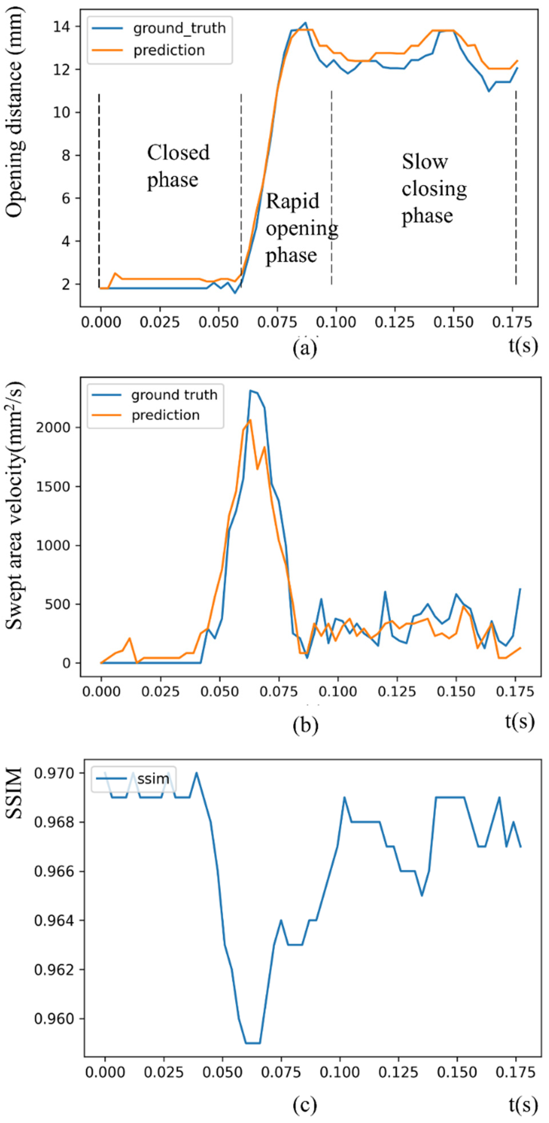
Furthermore, by comparing the results of image similarity metrics in different phases, we found that the accuracy varied depending on the phases. The most significant difference among phases is velocity: aortic valves in the rapid opening phase move faster than those in other phases. Therefore, velocity may affect the accuracy. The opening distance profile, the swept area velocity profile, and its corresponding SSIM accuracy profile are shown as an example of predicted motion and ground truth in Figure 7. In the figure, we can find that the predicted swept area velocity profile can roughly fit the ground truth. Furthermore, by combining these images, we found that the SSIM accuracy tends to decrease as the swept area velocity increases.

The reasons for these phenomena can be traced back to the CT imaging process. The higher the velocity is, the less significant the blur left by the motion image at that moment in the motion-blurred CT image. Motion-blurred CT images are reconstructed by projection data of different motion images from different projection angles at different times. The pixels in the motion-blurred CT image are related to the corresponding pixels in the motion images. Due to the motion of aortic valves, these pixels in the motion images switch between the material of blood and aortic valves, resulting in a blur in the motion-blurred CT images. To make a pixel more like the aortic valve, there must be multiple motion images in which the corresponding pixel is an aortic valve. When a motion image has high velocity, there are fewer shared pixels with adjacent motion images. Therefore, it is difficult to determine whether these pixels in motion-blurred CT images are aortic valves. Therefore, the blur left by the fast-moving motion image is insignificant.

Since velocity influences the accuracy, we further explored the velocity limitation of the trained model. We quantitatively evaluated the relationship between the swept area velocity and SSIM (

Table 11. The swept area velocity and SSIM.

Swept Area Velocity (mm2/s)	SSIM	Swept Area Velocity (mm2/s)	SSIM
0–200	0.974	1200–1400	0.965
200–400	0.972	1400–1600	0.963
400–600	0.971	1600–1800	0.962
600–800	0.970	1800–2000	0.962
800–1000	0.968	2000–2200	0.962
1000–1200	0.966	2200–2400	0.962

). We found that predicted images with the SSIM above 0.964 were very close to the ground truth images using empirical judgment. Therefore, our trained model can handle area swept velocity below 1400 mm²/s.

4.2. Interpretation of Motion Feature Evaluation Metrics

To evaluate the ability of the trained model to predict motion features, we must know that the average maximum opening distance of the test dataset is 12.4 mm, the average maximum-swept area velocity of the test dataset is approximately 1888.5 mm²/s, and the time for the CT simulator to generate one CT image is 183.3 ms. Based on the results in Table 7, the MDE is approximately 5.7% of the average max opening distance, the MVE is approximately 20.8% of the average maximum-swept area velocity, and the OTE is approximately 3.0% of the time for the CT simulator to generate one CT image. From the results, it was found that the trained DNN can infer opening time with a high accuracy. The high accuracy in inferring opening time confirmed that motion blur in CT images had temporal information of motion. Furthermore, we found that the trained DNN had some ability in inferring opening distance and maximum swept area velocity. The reasons for poor accuracy in terms of maximum swept area velocity is because of the relationship between velocity and accuracy and the velocity limitation of the trained DNN. Although there are still errors, considering the elusive motion information in the motion blur and the difficulty of dynamic imaging, these results are acceptable and a significant improvement over the results of traditional methods, which only extracted one sharp image from a motion-blurred CT image. In addition, we found that the trained model has some ability to distinguish different motions by analyzing the data distribution of maximum opening distance and maximum-swept area velocity. The average maximum opening distance and maximum-swept area velocity of prediction were close to the ground truth (Table 10). We can tell the difference between these eight motions based on their mean values. However, a large deviation in the data distribution is shown in Figure 6a,b. These data shows that the trained model required the mean value of multiple samples to distinguish different motions.

Our trained model had some ability to acquire accurate maximum opening distance, maximum-swept area velocity, and even the swept area velocity profile. Since the motions were varied by changing the geometric parameters and material properties, we further explored the relationship between these parameters and motion features. Geometric parameters affect the turbulence around aortic valves, whereas the material properties affect the bending stiffness and ductility of aortic valves. The geometric parameters can be easily measured from CT images of aortic valves in the closed phase, but it is difficult to evaluate the material properties of aortic valves. However, the detailed motion features obtained based on the proposed method can provide a new possibility for the evaluation of the material properties of aortic valves, inferring material properties from detailed motion features. There is a definite physical relationship between motion and material properties. Inferring material properties from detailed motion features can be considered an ill-posed problem with solutions, such as deep learning. Similar studies have been performed in other fields. Davis A, et al. [38] proposed a method to infer material properties from small motion in video and Schmidt F, et al. [39] integrated shape, motion, and optical cues to infer stiffness of unfamiliar objects. With the above studies, we conclude that the material properties of aortic valves can be evaluated using the detailed motion features obtained from the proposed method.

4.3. Model Generalization Evaluation

The trained model was evaluated using a test dataset. However, the accuracy of the trained model depends on the test dataset, making the results unreliable. Therefore, the generalizability of the DNN model should be evaluated. K-fold cross-validation [40] solves this problem by dividing the dataset into k numbers of subsets and ensuring that each subset is used as a test dataset at different folds, which ensures that our model does not depend on training and test datasets.

The dataset was split into four folds (Figure 8). In the first iteration, the first fold was used to test the model, and the rest were used to train the model. In the second iteration, the second fold was used as the testing dataset, while the rest served as the training dataset. This process was repeated until each fold of the four folds was used as a test set.

After k-fold cross-validation, SSIM and PSNR were calculated. As shown in

Table 12. Results of four-fold cross-validation.

	SSIM	PSNR
Fold 1	0.988 ± 0.005	36.534 ± 1.464
Fold 2	0.990 ± 0.004	37.267 ± 1.396
Fold 3	0.989 ± 0.003	36.921 ± 1.286
Fold 4	0.990 ± 0.003	37.486 ± 1.219
Average	0.989 ± 0.004	37.052 ± 1.341

, the accuracy is similar in all four folds, indicating the generalizability of the proposed DNN architecture. It also means that our algorithm is consistent, and we can be confident that by training it on the dataset generated with other simulation parameters can lead to similar performance.

4.4. Failure Cases

Figure 5b shows that the model failed to predict images in the rapid opening phase for some cases. The probability distribution of the failed cases is shown in Table 5. After analyzing the predicted motion images, we found that the failed cases were concentrated in the data generated from motion 3 and in the rapid opening phase of the aortic valve. In motion 3, the aortic valve thickness is 0.24 mm, and the velocity is fast because of the thin thickness. The intensity of the motion blur is related to the thickness of the aortic valve. Since the spatial resolution of the CT image is 0.5 mm/pixel, thin thickness indicates a low intensity of motion blur in the CT images. Therefore, the low intensity of motion blur could be the cause of this failure. Furthermore, in the failed cases in the rapid opening phase, the velocity of the rapid opening phase is higher than other phases. As previously stated, the higher the velocity is, the lower the accuracy. Therefore, one possible reason for this failure is the complexity of inferring motion images in the rapid opening phase. To improve the performance, it is necessary to increase the number of training data and use a more complex DNN architecture.

4.5. Study Limitations

Our study has proven the feasibility of the proposed concept in 2D under simulation conditions. However, it has potential limitations. Firstly, our study is limited to 2D. The 3D case will be more complicated because of the spatial motion as well as the arrangement of CT volume. It may be difficult to determine whether the motion blur is caused by the spatial motion or planar motion, and the arrangement of CT volume increased the complexity of the imaging process. Secondly, our study is conducted under simulation conditions. There is no real data involved. In our simulation, only motion blur generated by a specific reconstruction algorithm was considered. However, real data comprise several noise types, such as beam hardening and hardware-based noises. These noises may add useful information or affect the recognition of motion blur. Furthermore, there are many CT reconstruction algorithms, such as iterative and DNN reconstruction algorithms, and different reconstruction algorithms will make the motion blur pattern a little different. In the simulation, it is difficult to perfectly represent real physical processes. Simulation comes with simplified simulation models, such as the direction of CT imaging, linear elastic material properties of aortic valves, and incompressible Newtonian fluid of blood flow. In addition, the DNN model and the loss function we used are not optimized, so further improvements are required in future study.

Despite these limitations, we thought the simple simulation condition was sufficient to prove the proposed concept. Although it cannot perfectly reproduce the complex real-world situation, our study included the necessary variables and complexity of actual problems. Even in this simple in silico experimental setting, the motion simulator included the projection and reconstruction process of CT imaging, and the motion simulator included two-way fluid structure interaction. To verify how the proposed method can deal with varieties of valve motion, the material and geometric properties of aortic valves were varied in the motion simulator, and the CT imaging start times were varied in the CT simulator. Therefore, we considered the generated dataset sufficient to prove the proposed concept.

5. Conclusions

In this study, we have validated a concept that motion images can be inferred from motion blur in CT images of aortic valves under simulated conditions. The proposed method differs from previous methods for suppressing or removing motion blur. It will aid in the accurate diagnosis of aortic valves and the appropriate use of motion blur in the CT imaging field. Sixty motion images have been successfully inferred from a single motion-blurred CT image in 2D. The predicted images were evaluated with two image similarity evaluation metrics, SSIM (0.97 ± 0.01) and PSNR (36.0 ± 1.3 dB), and three motion feature evaluation strategies, the MDE between endpoints (0.7 ± 0.6 mm), the MVE between adjacent images (393.3 ± 423.3 mm²/s), and the OTE (5.5 ± 5.5 ms). The preliminary in silico learning results show a promising future for using deep learning techniques to learn motion information from motion-blurred CT images. Moreover, we found that the higher the velocity is, the lower the accuracy, so the predicted motion images may be useful in estimating the material properties of aortic valves.