Abstract
Orthogonal transformations, proper decomposition, and the Moore–Penrose inverse are traditional methods of obtaining the output layer weights for an extreme learning machine autoencoder. However, an increase in the number of hidden neurons causes higher convergence times and computational complexity, whereas the generalization capability is low when the number of neurons is small. One way to address this issue is to use the fast iterative shrinkage-thresholding algorithm (FISTA) to minimize the output weights of the extreme learning machine. In this work, we aim to improve the convergence speed of FISTA by using two fast algorithms of the shrinkage-thresholding class, called greedy FISTA (G-FISTA) and linearly convergent FISTA (LC-FISTA). Our method is an exciting proposal for decision-making involving the resolution of many application problems, especially those requiring longer computational times. In our experiments, we adopt six public datasets that are frequently used in machine learning: MNIST, NORB, CIFAR10, UMist, Caltech256, and Stanford Cars. We apply several metrics to evaluate the performance of our method, and the object of comparison is the FISTA algorithm due to its popularity for neural network training. The experimental results show that G-FISTA and LC-FISTA achieve higher convergence speeds in the autoencoder training process; for example, in the Stanford Cars dataset, G-FISTA and LC-FISTA are faster than FISTA by 48.42% and 47.32%, respectively. Overall, all three algorithms maintain good values of the performance metrics on all databases.
1. Introduction
In pattern recognition systems, efficient methods of feature selection and extraction can reduce the dimensionality problem, thus reducing both the computation time and the memory requirements of the training algorithms [1]. An autoencoder is a feed-forward neural network that builds a compact representation of the input data, and is mainly used for unsupervised learning [2]. It is composed of an encoder and a decoder: the encoder reads the input data and maps them to a lower-dimensionality space, while the decoder reads the compact representation and reconstructs the neural network input. In the same way as for all supervised learning neural networks [3,4], the core aspect of the training of an autoencoder is the backpropagation algorithm. This algorithm iteratively tunes the weights and biases of the neural network by applying the gradient descent method. Autoencoder networks are in great demand in multiple applications in modern society, for example, for dimensionality reduction, image retrieval, denoising, and data augmentation [2].
Several works in the literature have developed feature extraction methods using autoencoders and backpropagation. A comparative study between the performance of a traditional autoencoder and a denoising sparse autoencoder is presented in [5]. Another widely used architecture is the stacked autoencoder, which includes the stacked denoising sparse autoencoder [6] and the symmetric stacked autoencoder with shared weights [7]. Semi-supervised learning algorithms have also been used as autoencoder training algorithms [8,9]. However, the backpropagation training technique limits the generalization ability of the autoencoder, which results in low computational efficiency and the presence of local optima.
An extreme learning machine (ELM) is an emerging training paradigm for neural networks which includes supervised [10], semi-supervised [11], and unsupervised training [12]. The fundamental principle of this architecture is the random assignment of weights and biases in the hidden layer and the analytical determination of the weights of the output layer, in which the least squares method is applied to a system of linear equations [13,14]. The simplicity of the model, the lower numbers of training parameters, the low convergence speed, and its high generalization capacity mean that ELM neural networks have advantages for classification, regression, and clustering problems. Variants such as the kernel-ELM (K-ELM) [15], due to the significant reduction in the number of parameters and the increase in the training speed, and the online sequential ELM [16], due to its capacity to process batches of data, can even deal efficiently with problems involving large volumes of data. In the field of rolling element fault diagnosis, ELM can also solve the problem of weak signals caused by long transmission paths [17]; for example, the novel method presented in [18] can help in frame feature selection for ELM. In computer vision, the researchers of [19] proposed a visual object tracking scheme with promising results.
On the other hand, to handle the problems that local minima can cause, some studies have used heuristic optimization techniques to estimate the network parameters, such as differential evolution, particle swarming (PSO), and genetic algorithms [20]. These heuristic algorithms always search for the global minimum of the objective function and are efficient in several research fields, as is the case for the PSO algorithm that adjusts the parameters of an underactuated surface search model [21]. An improved scheme of this method integrates the PSO with global optimization capability, a 3-Opt algorithm with local search capability, and a fuzzy system with fuzzy reasoning ability [22]. The probabilistic ant colony algorithm is another optimization technique integrated into the architecture of an ELM network [23]. The K-ELM method improves the hyperspectral image classification capacity by coupling the principal component analysis, local binary pattern, and gray wolf optimization algorithm with global search capability [24].
Due to the advantages of ELM over backpropagation, the authors of [25] proposed to train autoencoder networks using an extreme learning machine (ELM-AE). A sparse ELM-AE was presented in [26] by adding the -norm in the quadratic term to give a more significant representation of data. Another approach for unlabeled feature extraction consisted of a generalized ELM-AE in which a manifold regularization factor was added to the objective function of the ELM-AE [27]. An unsupervised learning ELM-AE was proposed in [28], inspired by the use of embedding graphs to capture the structure of the input patterns, and was constructed using local Fisher discrimination analysis. A dense connection autoencoder was introduced into multi-layer learning, in which the output features of the previous layers were used by the following layers [29]. A double random hidden layer ELM autoencoder can achieve efficient extraction of features with dimension reduction capability for deep learning [30]. The -norm regularization has been used for the ELM-AE optimization problem, creating a new unsupervised learning framework that included a disperse representation despite the influence of atypical values and noisy data [31]. In addition, the correntropy-based ELM autoencoder presented in [32] was developed to extract features from noisy input patterns. To lower the number of parameters to be tuned and for the efficient calculation of the pseudo-inverse matrix, an ELM-AE with a kernel function was proposed in [33,34]. From a different perspective, the need for unsupervised batch learning means that an online sequential ELM-AE [35,36] is an exciting approach to solving large-scale applications.
From the works described above, we see that the backpropagation method and the Moore–Penrose inverse are two classical methods of estimating the weights of an autoencoder network. However, using these methods may cause overfitting when the number of unknown variables is larger than the number of training data. In addition, the accuracy is low when the number of hidden neurons is small, and the training time increases significantly when solving higher-dimensional applications. To overcome these drawbacks, researchers have proposed the use of sparse regularization techniques [37], with FISTA being the most widely used algorithm [38]. Although its origin dates back to 2009, this algorithm is still under study, thanks to its convergence speed, accuracy, and straightforward implementation. Several state-of-the-art studies have demonstrated the successful use of this optimization tool in machine learning. For example, in multilayer network design, the minimization problem defined in the autoencoder uses shrinkage-thresholding optimization techniques for dimension reduction and sparse feature representation [26,32,39]. For noisy image and video processing, a mixed scheme was presented in [40], in which sparse coding was adopted with deep learning to solve supervised and unsupervised tasks. A visual dictionary classification scheme was addressed in [41] using a simple (deep) convolutional autoencoder, for which the source of inspiration was sparse optimization and the iterative shrinkage-thresholding algorithm [38]. More recent studies [42,43] have demonstrated this algorithm’s development, continuity, and importance for solving convex minimization problems. In particular, they estimated the output weights of ELM and validated their results on classification problems.
Due to the importance of sparse regularization in the mathematical modeling of many real situations and the ability of shrinkage-thresholding algorithms to minimize these optimization problems, our work aims to study these optimization techniques in the architecture of an ELM-AE since there are few studies in the literature. Specifically, this paper proposes the use of fast algorithms from the shrinkage-thresholding family to improve the convergence speed achieved by FISTA during the training of an ELM-AE. In particular, two representative models of this class are considered: G-FISTA [44] and LC-FISTA [45,46]. To evaluate the efficiency of our scheme, six datasets that are widely used in the validation of ELM algorithms are adopted: MNIST, NORB, CIFAR10, UMist, Caltech256, and Stanford Cars. The main contributions of our article are as follows:
- We present a novel method for computing the output layer weights of the ELM-AE network that avoids the need for the Moore–Penrose inverse. Instead of solving the linear system analytically, we use first-order iterative algorithms from the class of shrinkage-thresholding algorithms to minimize the output weights of the ELM-AE.
- We demonstrate experimentally that the proposed method can effectively improve the computational time of the FISTA algorithm while maintaining its generalization capability. According to the theory presented in [47], the ELM-AE experiences a better performance when it achieves the lowest training error.
- Compared to FISTA, the G-FISTA, and LC-FISTA algorithms show a considerable improvement in the training time of the ELM-AE, for all of the databases, and a very competitive reconstruction capability. Thus, applying this mathematical tool in other contexts would constitute a significant scientific contribution.
The rest of this work is structured as follows: in Section 2, we briefly explain the ELM-AE, FISTA, G-FISTA, and LC-FISTA algorithms. Section 3 describes the method proposed to train the ELM-AEs. The datasets and the results are presented in Section 4. The discussion of results is presented in Section 5. Finally, Section 6 gives the conclusions of this work.
2. ELM-AE and Shrinkage-Thresholding Algorithms
2.1. Extreme Learning Machine Autoencoder
The ELM-AE [25] is trained with an ELM algorithm [10] in an unsupervised manner. It corresponds to a single hidden layer feedforward neural network, in which the outputs match the inputs. The ELM-AE has both a high training speed and a strong generalization ability due to the pseudo-random creation of neurons in the hidden layer and the application of a pseudoinverse matrix to calculate the weights of the output layer. To improve the performance of this method, the authors of [25] assigned random orthogonal weights and biases to the hidden layer. This approach was shown to have good generalization, and to minimize and the square norm of the coefficients . Given a set of N training samples , where are both the input and output data, the output with L hidden neurons can be expressed as follows:
where and represent the pseudorandom weights and biases of the hidden layer, g is an activation function, and represents the weights of the output layer. The previous overdetermined linear system can be compactly described as follows:
where is the hidden layer output matrix, is the output layer weight matrix, and is the input data matrix.
Indeed, is the standard solution to the overdetermined problem in (2), where is the Moore–Penrose inverse of matrix . To improve the performance of an ELM-AE, the authors of [25] determined the output weights by means of the equation , which is the result of solving the following regularized optimization problem:
where is a tuning regularization parameter.
2.2. The Shrinkage-Thresholding Class of Optimization Algorithms
A large number of applications can be formulated as a convex optimization problem [48], as shown by the following expression:
where are two convex functions, is -Lipschitz continuous and is a non-differentiable function that cannot be easily minimized in several machine learning applications. The solution to can be evaluated using the proximal operator [48], as shown in the following equation:
where is the stepsize and is the initial estimate of the solution. As a consequence, the optimization of the function h uses a two-phase method: (i) performance of a forward gradient descent step on the smooth function f; and (ii) performance of the proximal operator or a backward gradient descent step on the non-smooth function .
In the following, a brief description of the FISTA, G-FISTA, and LC-FISTA algorithms is presented. These algorithms can be used to train ELM-AEs.
2.2.1. Fast Iterative Shrinkage Thresholding Algorithm
FISTA [38] is characterized by its convergence speed and high level of efficiency. When minimizing the convex problem in (4), the algorithm has a convergence rate on the order of . The sequence of steps of the FISTA algorithm is as follows:
- (1)
- Update: .
- (2)
- Execute the intermediate step: .
- (3)
- Update: .
The term represents the step size, and represents the impulse factor. FISTA’s convergence rate depends mainly on its proximal operator and the use of a weighted step , which is expressed as a combination of both and . In addition, the configuration of the Lipschitz constant of the gradient f plays an essential part in the convergence of the algorithm.
2.2.2. Greedy FISTA
In general terms, G-FISTA [44] is a variant of FISTA that is characterized by a higher speed. Given the conditions imposed by G-FISTA, its architecture can restart the FISTA algorithm with the fixed impulse factor . This algorithm updates the solution to the optimization problem in (4), setting , and until the maximum number of iterations is reached. The updating scheme is as follows:
- (1)
- Update: .
- (2)
- Update: .
- (3)
- Restart: if , then .
- (4)
- Safeguard: if , then .
The G-FISTA algorithm improves the convergence rate and the reconstruction capability of FISTA, which uses a self-adaptive restart and adjustment scheme to obtain an additional acceleration and alleviate the oscillation problem in the reconstruction process. Based on the results discussed in [44,49], G-FISTA has efficient performance when . For this reason, all experiments performed in this work were configured with , , and .
2.2.3. Linearly Convergent FISTA
LC-FISTA is an accelerated version of FISTA derived from the research in [45,46]. Under specific error conditions, LC-FISTA works with global linear convergence for a large group of real applications, which minimizes the formulation of the convex problem of the equation in (4). The iterative steps of the algorithm are as follows:
- (1)
- Set both , and , , y .
- (2)
- Update: .
- (3)
- Update: .
- (4)
- Update: .
With a mathematical analysis analogous to that presented in [45,46], the sequence generated by the LC-FISTA scheme exhibits a linear convergence rate, for fixed values of and . The practical use of LC-FISTA requires tuning parameters such as the strong convexity parameter for the differentiable function f. In addition, we need to set to obtain convergence rates similar to the accelerated variant of FISTA presented in [50]. It is common to set , since the location of the global minimum of the objective function h is not known.
Remark 1.
The proximal operator is the step that is common to FISTA, G-FISTA, and LCFISTA. This value is closer to the global minimum of h compared with the maximum descent step . Since causes oscillations in the FISTA scheme when it has a value of one, G-FISTA shortens the interval between two restarts by setting , which is an essential condition for G-FISTA to converge with fewer iterations. In LC-FISTA, the θ and α momentum terms incorporated in the two additional equations (see (1) and (3) for LC-FISTA) improve both the accuracy of the gradient and the speed of convergence of LC-FISTA via the proximal operator.
3. Proposed Method of Training ELM-AEs Based on G-FISTA and LC-FISTA
ELM-AE has an extremely fast training speed, and good pattern reconstruction capability that is better than backpropagation-based learning. The formulation of this model can be expressed as a convex optimization problem which involves minimizing the weights of the output layer, as shown in the following equation:
where , and is a control parameter between the training error and the generalization ability.
Several methods exist for computing the solution to (6), such as the Moore–Penrose inverse, orthogonal projection, and proper decomposition [51]. However, in a real situation, the number of independent variables L in the linear system is much larger than the number of data points N, which may cause overfitting. On the other hand, the reconstruction capacity is low whenever the number of hidden neurons L is small. As the training dataset increases, the computational cost of the inverse matrix increases significantly. Several regularization methods have been introduced in the literature to address the above problems. The two most commonly used classical techniques are ridge regression [52] and sparse regularization [37]. The sparse regularization plays an important role in feature selection, which has shown successful results in machine learning. This study presents an unsupervised feature selection framework, which integrates sparse optimization and signal reconstruction for pattern recognition models. The minimization problem takes the following form:
which is a special case of (4), in which we set and .
From the description given above, we see that the estimation of and the time required are the main challenges for training the ELM-AE. Our study proposes two novel iterative schemes for autoencoder training, G-FISTA, and LC-FISTA, which reduce the computational time of FISTA maintaining its accuracy, where FISTA is the classical algorithm for training neural networks. This optimization approach is also interesting because it can be extended to other regularization terms, which control the variables selection by calculating a derivative in the weakest sense through convex envelopes. In addition, the closed form of the proximal operator of is computed by the shrinkage operator [38], whose i-th element is calculated as follows:
where is the initial estimation of the weight of the output layer.
The speed that can be achieved by the use of G-FISTA and LC-FISTA in the training of the ELM-AE is significantly higher than that obtained using FISTA. In addition, for poorly conditioned matrices, the two algorithms have the same ability as FISTA to reconstruct the input signals. This is realized by the omission of several steps of the gradient descent, and correction of the solution by means of the proximal gradient. Although the iterative scheme used by G-FISTA and LC-FISTA effectively has additional terms compared to FISTA, the computational cost can be similar, since they converge with fewer iterations. The following algorithm presents the steps that are followed in the training of the ELM-AE, where the parameters to be configured are the number of iterations I, the number of neurons L, the stopping criterion P and the regularization parameter . The variables represent features associated with the pixels of the images, ordered according to the columns of the matrix . In the reconstruction and variable selection process, the input data, expected target, network weights, and biases are matrix arrays that facilitate the computation of many vector operations.
4. Experimental Evaluation
This section presents the databases and evaluation metrics selected to evaluate the performance of the proposed method.
4.1. Hardware, Software and Databases
For this work, a server from the cluster of the Laboratory of Technological Research in Pattern Recognition (LITRP) of the Universidad Católica del Maule was used. The server was equipped with two CPUs, an Intel Xeon Gold 6238 252 CPU @ 2.20–4.00 GHz (56 physical cores), 126 GB RAM and a GPU NVIDIA Titan RTX. The algorithms were implemented in the MATLAB R2020a programming language.
To examine the performance of Algorithm 1, we used the CIFAR10, UMist, MNIST, NORB, Stanford Cars and Caltech256 databases, which were obtained from different free online repositories. These datasets are briefly described below.
- (1)
- MNIST. This dataset contains 70,000 images of handwritten digits from zero to nine. These are grayscale images of size pixels which generate a vector of 784 components.
- (2)
- NORB. This consists of 48,600 grayscale stereo images of 50 toys from five generic classes: cars, four-legged animals, human figures, airplanes, and trucks. The size of the images is pixels, and the output is a vector of = 18,432 components.
- (3)
- CIFAR10. This dataset consists of 60,000 color images distributed into 10 classes: airplanes, birds, automobiles, cats, dogs, frogs, deer, ships, horses, and trucks. The number of images per class is 6000, with 5000 used for training and the remainder for testing. In this experiment, the color images were converted to grayscale and had a size of pixels.
- (4)
- UMist. This contains 575 grayscale images of 20 people, showing individuals in different positions. The images are rectangular, with a size of pixels.
- (5)
- Caltech256. This dataset contains 30,607 color images grouped into 257 categories, each of which contain at least 80 images. For the purposes of this study, the images were converted to grayscale and had a size of pixels.
- (6)
- Stanford Cars (SCars). The Stanford Cars dataset contains 16,185 images of 196 categories of automobiles. For training, the color images were converted to grayscale images of size pixels.
| Algorithm 1 Training of the ELM-AE with FISTA, G-FISTA, and LC-FISTA. |
| Require: training set , maximum number of iterations I, stopping criterion P, number of neurons L, regularization parameter . 1: Random and orthogonal assignment of weights and biases in the hidden layer. 2: Calculation of the matrix evaluating g in the terms . 3: while P does not occur do 4: Calculate the optimal value of (4) using the G-FISTA or LC-FISTA algorithms for and . 5: end while |
Table 1 shows the numbers of training and test data, the numbers of categories, and the sizes of the input vectors for CIFAR10, UMist, MNIST, NORB, Stanford Cars, and Caltech256.

Table 1.
Information from the databases to train the ELM-AE.
4.2. Selection of Evaluation Metrics
To analyze the performance of the proposed algorithm, we used the root mean square error (RMSE), mean absolute error (MAE), score, index of agreement (AI), Theil inequality coefficient (TIC), minimum error (MIN), and maximum error (MAX), as defined in Table 2 [53]. We used the RMSE and MAE metrics to represent the average error between the estimated and actual values. The lower the values of these measures, the higher the efficiency of the autoencoder.
Table 2.
Seven evaluation criteria to evaluate the performance of the proposed method.
The score is a statistical measure that is defined on the domain , where a value of one indicates perfect prediction and zero an inefficient model [54]. In contrast, the TIC metric indicates the accuracy capability of the proposed system, with a value between zero and one. The closer the value is to zero, the higher the predictive efficiency of the ELM-AE method. Likewise, the IA prediction index can provide external statistical information on the predictive ability of the model. To verify the efficiency of the ELM-AE, each experiment was repeated 10 times, and the average values of the training times and the evaluation criteria represented in Table 2 were recorded.
4.3. Experimental Setup
In each experiment, the training and test data were standardized to the range using the following equation:
where is the actual value to be standardized, and are the minimum and maximum of the actual values. In the hidden layer, the weights and biases are random values generated by means of a uniform distribution in the ranges and , and the sigmoid was used as the activation function. We chose this activation function due to its universal approximation capability in ELM networks.
The algorithm presented in Section 3 has the following parameters that need to be configured: the number of neurons L, the stopping criterion P, the maximum number of iterations I, and the regularization term . In the first scenario of the proposed method, the regularization parameter set to , the stopping criterion P is expressed as and the maximum number of iterations is . The threshold is a user-specified value that is applied to interrupt the iteration of the algorithm. For the UMist, CIFAR10, MNIST, NORB, SCars, and Caltech256 databases, we set and , respectively. Moreover, the practical application of the FISTA, G-FISTA, and LC-FISTA algorithms for training of the ELM-AE requires tuning of the Lipschitz constant, and the strong convexity constant must be tuned for the LC-FISTA algorithm. For the convex function , we chose values of and , where and are the minimum and maximum proper values of . The additional control parameters in G-FISTA were described in Section 2.2.2.
In a second scenario, we evaluated the sensitivity of the regularization parameter on the performance of our method for the UMist, NORB, Stanford Cars, and Caltech256 datasets. This tuning term was chosen using cross-validation for each algorithm and database. Table 3 shows the optimal value of selected of , obtained by comparing the RMSE between the generated models, chosen as the that gives a lower RMSE. The experiment only considered the case for the selected databases. The other parameters of the FISTA, G-FISTA, and LC-FISTA algorithms follow the same selection criteria of the first scenario. For example, the steplength for FISTA and LC-FISTA has been , but for G-FISTA, , , and . The Lipschitz constant and the strong convexity parameter of f are taken as the maximum and minimum eigenvalue of the matrix . The mathematical analysis and numerical experiments presented in [42,43,44,45,49] motivated the choice of our parameters.
Table 3.
Choice of for each algorithm and selected database.
To avoid the problem of overfitting when the number of neurons is increased, we applied a 10-fold cross-validation technique. This control tool allowed us to restrict the training to a certain number of neurons. We then used the test set specified in Table 1 and the metrics defined in Table 2 to evaluate the performance of each algorithm. Figure 1 shows the values of the RMSE for the training, validation, and test sets for the G-FISTA algorithm. A graphical view is not shown for FISTA and LC-FISTA since all three algorithms had a comparable level of accuracy. According to the above analysis, and were the maximum neuron thresholds that could be assigned in ELM-AE for the MNIST and CIFAR10 databases.
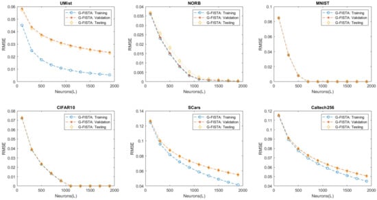
Figure 1.
G-FISTA Algorithm: plot of RMSE for training, validation, and testing sets versus the number of neurons.
4.4. Representation of Features with Different Numbers of Neurons
The computational complexity and execution time of the proposed method are explored in this section. For this purpose, several cases are considered with varying numbers of neurons in the hidden layer of the ELM-AE. In this phase of the experiments, we selected the measures of training time, RMSE, MAE, , IA, TIC, MIN, and MAX for comparison on the test set. These evaluation indicators were obtained as a result of training the ELM-AE with the shrinkage-thresholding class of algorithms introduced in Section 2.2.
Table 4 presents the training times and values of RMSE for the ELM-AE on each of the six datasets, for increasing numbers of neurons in the hidden layer. These experimental results show that the training speeds achieved by G-FISTA and LC-FISTA were lower than that obtained by FISTA. For example, for the CIFAR10 set, with 100 neurons in the hidden layer, the computation time fo rthe ELM trained by FISTA was 21.92 s, while the G-FISTA and LC-FISTA algorithms achieved average values of 12.31 s and 12.91 s. Likewise, when we increased the number of hidden neurons , the training time obtained by G-FISTA and LC-FISTA was approximately half that required by FISTA. At the test stage, the RMSE metric achieved by the G-FISTA and LC-FISTA algorithms proposed in this paper indicated a similar level of error as the current FISTA algorithm. This evaluation metric became smaller as the parameter L was increased. For MNIST and CIFAR10, we obtained evaluation metrics of up to and , respectively.
Table 4.
Training times and RMSE values achieved by FISTA, G-FISTA, and LC-FISTA for training of the ELM-AE.
For each dataset, we show the execution time of the proposed method in Figure 2. A bar chart represents this evaluation measure as a function of the number of neurons. The blue, red, and orange bars indicate the training times obtained by FISTA, G-FISTA, and LC-FISTA, respectively. From the results illustrated in Figure 2, we infer that the proposed G-FISTA and LC-FISTA algorithms are faster than FISTA for training the ELM-AE.
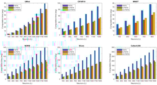
Figure 2.
Bar graph representing the average training times required by FISTA, G-FISTA, and LC-FISTA for the ELM-AE.
In the following, we demonstrate the efficiency of the proposed method using four evaluation criteria: the MAE, score, IA, and TIC. A summary of the MAE and values is given in Table 5. The closer the value of MAE to zero, and the closer the value of to one, the better the performance of the autoencoder. From the values of the metrics given in Table 5, we can see that the order of magnitude is similar, and there is no significant difference between the shrinkage-thresholding methods, meaning that the proposed method maintains the same level of accuracy as the FISTA algorithm. Taking the UMist database as an example, we see that when , the average MAE values obtained by FISTA, G-FISTA, and LC-FISTA are 0.0172, 0.0181, and 0.0178, while their scores are 0.9861, 0.9846, and 0.9851, respectively. The IA and TIA metrics are also important for evaluating the capability of the proposed learning system. These fit metrics are described in Table 6. As the average values of the IA and TIA approach one and zero, respectively, the feature representation improves.
Table 5.
MAE and score values achieved by FISTA, G-FISTA and LC-FISTA for training of the ELM-AE.
Table 6.
IA and TIA values achieved by FISTA, G-FISTA and LC-FISTA for training of the ELM-AE.
Table 7 shows the MIN and MAX statistical indices for the proposed model on all the selected databases. This table indicates the minimum and maximum absolute errors for the ELM-AE in the testing stage. From the results of this experimental analysis, we can conclude that the FISTA algorithm has a similar generalization capability as G-FISTA and LC-FISTA.
Table 7.
MIN and MAX values achieved by FISTA, G-FISTA and LC-FISTA for training of the ELM-AE.
The best tuning of the parameter in ELM-AE usually influences its generalization capacity. With the in Table 3 chosen using cross-validation, we show in Table 8 the performance of our method for the particular case . The values of RMSE and the training time are the two indicators selected to compare the efficiency of FISTA, G-FISTA, and LC-FISTA in ELM-AE. The time shown in Table 8 is the execution time required to select the parameter . Note that G-FISTA and LC-FISTA maintain the reconstruction capability of FISTA but perform better in terms of computational time. In addition, the values of RMSE in Table 4 and Table 8 for the first and second scenarios are comparable measures. Therefore, the chosen in the first scenario and the additional parameters may be adequate in large-scale application problems since cross-validation is not required.
Table 8.
The performance of each algorithm for the chosen in Table 3.
5. Discussion
The main goal of an autoencoder is to learn a compressed representation of the input and then reconstruct it within a reasonable computation time. This study proposes a robust sparse optimization-based method for training ELM-AE networks. With the control parameters specified in the results section, we see that the training times for G-FISTA and LC-FISTA are less than for FISTA. Table 9 shows these important results in terms of percentages. For the CIFAR10, UMist, MNIST, NORB, SCars, and Caltech256 databases, the average computation times for G-FISTA are 44.48%, 14.42%, 35.87%, 42.97%, 48.42%, and 39.43% faster than for FISTA, respectively. The LC-FISTA algorithm achieved speedups of 42.41%, 18.71%, 27.70%, 47.93%, 47.32%, and 43.90%. In addition, the indicators recorded in Table 4, Table 5, Table 6, Table 7 and Table 8 are coherent, and show comparable performance for all databases. The proposed training scheme is an important automatic learning method since it can help make accurate decisions in shorter periods. Consequently, incorporating fast optimization techniques into the autoencoder architecture can help improve the performance of current models, and particularly the first-order methods of the shrinkage-thresholding class.
Table 9.
Average speeds of the G-FISTA and LC-FISTA algorithms compared with FISTA for training of the ELM-AE.
The proximal step of FISTA requires the main computational effort, and this also holds true for G-FISTA and LC-FISTA. The additional computation required in G-FISTA and LC-FISTA increases the convergence speed, but the execution cost is higher. However, this problem can be controlled, since G-FISTA and LC-FISTA converge with fewer iterations. In the experimental evaluation described in Section 4, we raised the complexity of the problem by increasing the number of neurons in the hidden layer to get a clearer idea of the performance when solving applications involving higher dimensional datasets. Based on this evaluation criterion, we see that the proposed method can be configured to solve large-scale problems, since the vector operations involved in the ELM-AE architecture and the proposed mechanism are block-separable.
6. Conclusions
This paper has proposed the G-FISTA and LC-FISTA algorithms to reduce the training time of ELM-AEs. The performance of our methods was compared to FISTA, an algorithm of the shrinkage-thresholding class, which is a state-of-the-art method of training ELM-AEs.
Experiments were conducted on six databases: CIFAR10, UMist, MNIST, NORB, Stanford Cars, and Caltech256. The results showed that G-FISTA and LC-FISTA achieved similar computational times for the training of the autoencoder, both of which were significantly lower than FISTA. In numerical terms, G-FISTA and LC-FISTA were 37.60% and 37.99% faster than FISTA in training the ELM-AE (average value obtained from Table 9). Consequently, the advantage main of our study is to maintain the generalization capability of FISTA while the computational speed is improved. A possible disadvantage may be the hyperparameter settings, but many researchers set these values according to existing mathematical analysis in the literature to control runtime. Other advantages and disadvantages we will discuss in future perspectives.
Motivated by technological advances and the speed of convergence of shrinkage-thresholding algorithms, we intend to extend our methodology in further research to a parallel and distributed architecture. This approach will be of great interest for solving current large-scale applications in computer clusters and clouds. In addition, we aim to incorporate iterative schemes of the shrinkage-thresholding class into the architecture of a variational, convolutional deep autoencoder network to solve optimization problems with large datasets.
Author Contributions
Conceptualization, J.A.V.-C., M.M. and K.V.; methodology, J.A.V.-C. and M.M.; software, J.A.V.-C.; experimental execution and validation, J.A.V.-C.; research, J.A.V.-C., M.M. and K.V.; resources, M.M.; writing—review and editing, J.A.V.-C., M.M. and K.V.; scientific project coordination, M.M. and K.V.; funding acquisition, M.M. All authors have read and agreed to the published version of the manuscript.
Funding
This research was partially funded by Universidad Católica del Maule Doctoral Studies Scholarship 2019 (Beca Doctoral Universidad Católica del Maule 2019).
Institutional Review Board Statement
Not applicable.
Informed Consent Statement
Not applicable.
Data Availability Statement
Not applicable.
Acknowledgments
This paper is one of the scientific results of the project FONDECYT REGULAR 2020 N 1200810 Very Large Fingerprint Classification based on a Fast and Distributed Extreme Learning Machine, National Research and Development Agency, Ministry of Science, Technology, Knowledge and Innovation, Government of Chile.
Conflicts of Interest
The authors declare no conflict of interest. The funders had no role in the design of the study; in the collection, analyses, or interpretation of data; in the writing of the manuscript, or in the decision to publish the results.
Abbreviations
The following abbreviations are used in this manuscript:
| ELM | Extreme learning machine |
| ELM-AE | Extreme learning machine autoencoder |
| K-ELM | Kernel-ELM |
| FISTA | Fast iterative shrinkage-thresholding algorithm |
| G-FISTA | Greedy FISTA |
| LC-FISTA | Linearly convergent FISTA |
| RMSE | Root mean square error |
| MAE | Mean absolute error |
| R | R score |
| IA | Index of agreement |
| TIC | Theil inequality coefficient |
| MIN | Minimum error |
| MAX | Maximum error |
| PSO | Particle swarm optimization |
| CPU | Central processing unit |
| GPU | Graphics processing unit |
References
- He, X.; Ji, M.; Zhang, C.; Bao, H. A variance minimization criterion to feature selection using laplacian regularization. IEEE Trans. Pattern Anal. Mach. Intell. 2011, 33, 2013–2025. [Google Scholar] [PubMed]
- Dong, G.; Liao, G.; Liu, H.; Kuang, G. A review of the autoencoder and its variants: A comparative perspective from target recognition in synthetic-aperture radar images. IEEE Geosci. Remote Sens. Mag. 2018, 6, 44–68. [Google Scholar] [CrossRef]
- Leijnen, S.; Veen, F.V. The Neural Network Zoo. Proceedings 2020, 47, 9. [Google Scholar]
- Baldi, P.; Sadowski, P.; Lu, Z. Learning in the machine: Random backpropagation and the deep learning channel. Artif. Intell. 2018, 260, 1–35. [Google Scholar] [CrossRef]
- Meng, L.; Ding, S.; Xue, Y. Research on denoising sparse autoencoder. Int. J. Mach. Learn. Cybern. 2017, 8, 1719–1729. [Google Scholar] [CrossRef]
- Meng, L.; Ding, S.; Zhang, N.; Zhang, J. Research of stacked denoising sparse autoencoder. Neural Comput. Appl. 2018, 30, 2083–2100. [Google Scholar] [CrossRef]
- Li, R.; Li, S.; Xu, K.; Li, X.; Lu, J.; Zeng, M. A Novel Symmetric Stacked Autoencoder for Adversarial Domain Adaptation Under Variable Speed. IEEE Access 2022, 10, 24678–24689. [Google Scholar] [CrossRef]
- Luo, X.; Li, X.; Wang, Z.; Liang, J. Discriminant autoencoder for feature extraction in fault diagnosis. Chemom. Intell. Lab. Syst. 2019, 192, 103814. [Google Scholar] [CrossRef]
- Soydaner, D. Hyper Autoencoders. Neural Process. Lett. 2020, 52, 1395–1413. [Google Scholar] [CrossRef]
- Huang, G.B.; Zhu, Q.Y.; Siew, C.K. Extreme learning machine: Theory and applications. Neurocomputing 2006, 70, 489–501. [Google Scholar] [CrossRef]
- Huang, G.; Song, S.; Gupta, J.N.D.; Wu, C. Semi-Supervised and Unsupervised Extreme Learning Machines. IEEE Trans. Cybern. 2014, 44, 2405–2417. [Google Scholar] [CrossRef] [PubMed]
- Chen, J.; Zeng, Y.; Li, Y.; Huang, G.B. Unsupervised feature selection based extreme learning machine for clustering. Neurocomputing 2020, 386, 198–207. [Google Scholar] [CrossRef]
- Huang, G.; Huang, G.B.; Song, S.; You, K. Trends in extreme learning machines: A review. Neural Netw. 2015, 61, 32–48. [Google Scholar] [CrossRef] [PubMed]
- Huang, G.B.; Zhou, H.; Ding, X.; Zhang, R. Extreme learning machine for regression and multiclass classification. IEEE Trans. Syst. Man Cybern. Part B-Cybern. 2012, 42, 513–529. [Google Scholar] [CrossRef]
- Bai, Z.; Huang, G.B.; Wang, D.; Wang, H.; Westover, M.B. Sparse extreme learning machine for classification. IEEE Trans. Cybern. 2014, 44, 1858–1870. [Google Scholar] [CrossRef]
- Liang, N.Y.; Huang, G.B.; Saratchandran, P.; Sundararajan, N. A fast and accurate online sequential learning algorithm for feedforward networks. IEEE Trans. Neural Netw. 2006, 17, 1411–1423. [Google Scholar] [CrossRef]
- Ma, J.; Yu, S.; Cheng, W. Composite Fault Diagnosis of Rolling Bearing Based on Chaotic Honey Badger Algorithm Optimizing VMD and ELM. Machines 2022, 10, 469. [Google Scholar] [CrossRef]
- Cui, H.; Guan, Y.; Chen, H. Rolling element fault diagnosis based on VMD and sensitivity MCKD. IEEE Access 2021, 9, 120297–120308. [Google Scholar] [CrossRef]
- An, Z.; Wang, X.; Li, B.; Xiang, Z.; Zhang, B. Robust visual tracking for UAVs with dynamic feature weight selection. Appl. Intell. 2022. [Google Scholar] [CrossRef]
- Eshtay, M.; Faris, H.; Obeid, N. Metaheuristic-based extreme learning machines: A review of design formulations and applications. Int. J. Mach. Learn. Cybern. 2019, 10, 1543–1561. [Google Scholar] [CrossRef]
- Li, G.; Li, Y.; Chen, H.; Deng, W. Fractional-order controller for course-keeping of underactuated surface vessels based on frequency domain specification and improved particle swarm optimization algorithm. Appl. Sci. 2022, 12, 3139. [Google Scholar] [CrossRef]
- Zhou, X.; Ma, H.; Gu, J.; Chen, H.; Deng, W. Parameter adaptation-based ant colony optimization with dynamic hybrid mechanism. Eng. Appl. Artif. Intell. 2022, 114, 105–139. [Google Scholar] [CrossRef]
- Ali, M.; Deo, R.C.; Xiang, Y.; Prasad, R.; Li, J.; Farooque, A.; Yaseen, Z.M. Coupled online sequential extreme learning machine model with ant colony optimization algorithm for wheat yield prediction. Sci. Rep. 2022, 12, 5488. [Google Scholar] [CrossRef]
- Chen, H.; Miao, F.; Chen, Y.; Xiong, Y.; Chen, T. A hyperspectral image classification method using multifeature vectors and optimized KELM. IEEE J. Sel. Top. Appl. Earth Observ. Remote Sens. 2021, 14, 2781–2795. [Google Scholar] [CrossRef]
- Chamara, L.; Zhou, H.; Huang, G.B.; Vong, C.M. Representation learning with extreme learning machine for big data. IEEE Intell. Syst. 2013, 28, 31–34. [Google Scholar]
- Tang, J.; Deng, C.; Huang, G.B. Extreme learning machine for multilayer perceptron. IEEE Trans. Neural Netw. Learn. Syst. 2016, 27, 809–821. [Google Scholar] [CrossRef]
- Sun, K.; Zhang, J.; Zhang, C.; Hu, J. Generalized extreme learning machine autoencoder and a new deep neural network. Neurocomputing 2017, 230, 374–381. [Google Scholar] [CrossRef]
- Ge, H.; Sun, W.; Zhao, M.; Yao, Y. Stacked denoising extreme learning machine autoencoder based on graph embedding for feature representation. IEEE Access 2019, 7, 13433–13444. [Google Scholar] [CrossRef]
- Wang, J.; Guo, P.; Li, Y. DensePILAE: A feature reuse pseudoinverse learning algorithm for deep stacked autoencoder. Complex Intell. Syst. 2021, 8, 2039–2049. [Google Scholar] [CrossRef]
- Li, R.; Wang, X.; Lei, L.; Wu, C. Representation learning by hierarchical ELM auto-encoder with double random hidden layers. IET Comput. Vis. 2019, 13, 411–419. [Google Scholar] [CrossRef]
- Li, R.; Wang, X.; Song, Y.; Lei, L. Hierarchical extreme learning machine with L21-norm loss and regularization. Int. J. Mach. Learn. Cybern. 2021, 12, 1297–1310. [Google Scholar] [CrossRef]
- Liangjun, C.; Honeine, P.; Hua, Q.; Jihong, Z.; Xia, S. Correntropy-based robust multilayer extreme learning machines. Pattern Recognit. 2018, 84, 357–370. [Google Scholar] [CrossRef] [Green Version]
- Wong, C.M.; Vong, C.M.; Wong, P.K.; Cao, J. Kernel-based multilayer extreme learning machines for representation learning. IEEE Trans. Neural Netw. Learn. Syst. 2018, 29, 757–762. [Google Scholar] [CrossRef] [PubMed]
- Vong, C.M.; Chen, C.; Wong, P.K. Empirical kernel map-based multilayer extreme learning machines for representation learning. Neurocomputing 2018, 310, 265–276. [Google Scholar] [CrossRef]
- Paul, A.N.; Yan, P.; Yang, Y.; Zhang, H.; Du, S.; Wu, Q. Non-iterative online sequential learning strategy for autoencoder and classifier. Neural Comput. Appl. 2021, 33, 16345–16361. [Google Scholar] [CrossRef]
- Mirza, B.; Kok, S.; Dong, F. Multi-layer online sequential extreme learning machine for image classification. In Proceedings of ELM-2015 Volume 1; Springer: Berlin/Heidelberg, Germany, 2016; pp. 39–49. [Google Scholar]
- Tibshirani, R. Regression shrinkage and selection via the Lasso. J. R. Stat. Soc. B Methodol. 1996, 58, 267–288. [Google Scholar] [CrossRef]
- Beck, A.; Teboulle, M. A fast iterative shrinkage-thresholding algorithm for linear inverse problems. SIAM J. Imaging Sci. 2009, 2, 183–202. [Google Scholar] [CrossRef]
- Jiang, X.; Yan, T.; Zhu, J.; He, B.; Li, W.; Du, H.; Sun, S. Densely connected deep extreme learning machine algorithm. Cogn. Comput. 2020, 12, 979–990. [Google Scholar] [CrossRef]
- Zhao, H.; Ding, S.; Li, X.; Huang, H. Deep neural network structured sparse coding for online processing. IEEE Access 2018, 6, 74778–74791. [Google Scholar] [CrossRef]
- Liu, D.; Liang, C.; Chen, S.; Tie, Y.; Qi, L. Auto-encoder based structured dictionary learning for visual classification. Neurocomputing 2021, 438, 34–43. [Google Scholar] [CrossRef]
- Janngam, K.; Wattanataweekul, R. A New Accelerated Fixed-Point Algorithm for Classification and Convex Minimization Problems in Hilbert Spaces with Directed Graphs. Symmetry 2022, 14, 1059. [Google Scholar] [CrossRef]
- Chumpungam, D.; Sarnmeta, P.; Suantai, S. An Accelerated Convex Optimization Algorithm with Line Search and Applications in Machine Learning. Mathematics 2022, 10, 1491. [Google Scholar] [CrossRef]
- Liang, J.; Luo, T.; Schönlieb, C.B. Improving “Fast Iterative Shrinkage-Thresholding Algorithm”: Faster, Smarter, and Greedier. SIAM J. Sci. Comput. 2022, 44, A1069–A1091. [Google Scholar] [CrossRef]
- Bussaban, L.; Kaewkhao, A.; Suantai, S. Inertial s-iteration forward-backward algorithm for a family of nonexpansive operators with applications to image restoration problems. Filomat 2021, 35, 771–782. [Google Scholar] [CrossRef]
- Chambolle, A.; Dossal, C. On the convergence of the iterates of the “fast iterative shrinkage/thresholding algorithm”. J. Optim. Theory Appl. 2015, 166, 968–982. [Google Scholar] [CrossRef]
- Bartlett, P. The sample complexity of pattern classification with neural networks: The size of the weights is more important than the size of the network. IEEE Trans. Inf. Theory 1998, 44. [Google Scholar] [CrossRef]
- Beck, A.; Teboulle, M. Gradient-based algorithms with applications to signal recovery. In Convex Optimization in Signal Processing and Communications; Cambridge University Press: Cambridge, UK, 2009; pp. 42–88. [Google Scholar]
- Chen, L.; Xiao, Y.; Yang, T. Application of the improved fast iterative shrinkage-thresholding algorithms in sound source localization. Appl. Acoust. 2021, 180, 108101. [Google Scholar] [CrossRef]
- Calatroni, L.; Chambolle, A. Backtracking strategies for accelerated descent methods with smooth composite objectives. SIAM J. Optim. 2019, 29, 1772–1798. [Google Scholar] [CrossRef]
- Sun, P.; Yang, L. Generalized eigenvalue extreme learning machine for classification. Appl. Intell. 2022, 52, 6662–6691. [Google Scholar] [CrossRef]
- Tikhonov, A.N.; Arsenin, V.Y. Solutions of Ill-Posed Problems; V.H. Winston: Washington, DC, USA, 1977. [Google Scholar]
- Niu, X.; Wang, J.; Zhang, L. Carbon price forecasting system based on error correction and divide-conquer strategies. Appl. Soft. Comput. 2022, 118, 107935. [Google Scholar] [CrossRef]
- Hao, Y.; Niu, X.; Wang, J. Impacts of haze pollution on China’s tourism industry: A system of economic loss analysis. J. Environ. Econ. Manag. 2021, 295, 113051. [Google Scholar] [CrossRef] [PubMed]
Publisher’s Note: MDPI stays neutral with regard to jurisdictional claims in published maps and institutional affiliations. |
© 2022 by the authors. Licensee MDPI, Basel, Switzerland. This article is an open access article distributed under the terms and conditions of the Creative Commons Attribution (CC BY) license (https://creativecommons.org/licenses/by/4.0/).