A Novel Reliability Analysis Approach under Multiple Failure Modes Using an Adaptive MGRP Model

Abstract

In this paper, a novel MRGP-SS method is proposed to deal with the reliability analysis problems under multiple failure modes. First, a random moving quadrilateral grid sampling (RMQGS) method is proposed to improve the randomness and uniformity of initial samples. Second, an adaptive procedure, which combines the multiple response Gaussian process (MRGP) model and the novel active learning functions, is proposed to efficiently and accurately produce surrogate models for failure surfaces. In this regard, two novel learning functions are introduced to adapt to different iterative cycles, one is employed to correct the quality of samples, and the other is used to search for the samples closest to the limit state surface. Third, the subset simulation (SS) is integrated into the adaptive MRGP model to estimate the failure probability under multiple failure modes with fewer function calls and time consumption. Numerical and engineering case studies are finally provided to demonstrate the effectiveness of the proposed method.

1. Introduction

Reliability analysis aims at quantifying the reliability state of each performance index with the consideration of various sources of uncertainties, such as sizes, loads, accelerations, and variations in material properties. Generally, it can be divided into “system reliability analysis” (SRA) and “component reliability analysis” (CRA). The former means considering multiple failure modes, while the latter only considers one single failure mode [1,2].

For CRA, many methods have been developed to improve its efficiency, accuracy, and engineering applicability. They are divided into three categories according to their models. The first category is the approximate analytical method, which commonly adopts the most probable points (MPPs) to replace the mean point as the Taylor series expansion point of the limit state function [3]. Among them, the first-order reliability method (FORM) and the second-order reliability method (SORM) are the classical analysis methods based on MPP expansion. However, both of them need to normalize the non-normal random variables in the solution process, which increases the nonlinearity of the performance function. Thus, Du et al. [4] proposed the first-order saddlepoint approximation (FOSPA) method based on the maximum likelihood point model. Huang et al. [5] studied the mean value first-order saddlepoint approximation (MVFOSPA) method, which effectively improves the efficiency and robustness of the calculation. Different from the above methods, Rosenblueth [6] investigated the two-point estimation method. Gorman [7] performed a three-point estimation method considering the first four moments of the input variables. Wang et al. [8], Remennikov et al. [9], Zhang et al. [10], and Ngamkhanong et al. [11] presented some moment estimation methods, which enrich and improve the development of approximate analytical methods. The second category is the surrogate model-based method, which is widely investigated and used due to its strong fitting ability and small number of calculations. At present, the polynomial response surface method (RSM) [12,13], artificial neural networks (ANN) [14], radial basis function (RBF) [15], support vector machines (SVM) [16], polynomial chaos expansion (PCE) [17], and single response Gaussian process (SRGP) model (i.e., Kriging model) [18] are the classical surrogate models. Among these methods, the Kriging model has attracted the attention of many scholars because of its strong nonlinear fitting ability and generalization ability. It can be divided into the static surrogate model and the active learning (adaptive) surrogate model. The difference is that the former requires more initial sample points to ensure the approximation accuracy of the surrogate model, and the latter can continuously optimize the sample quality by adding new samples to update the model. Given the high fitting accuracy and efficiency of the adaptive Kriging surrogate model, its initial design point selection, update strategy, point addition scheme, probability evaluation, termination criterion, etc., have gained the most attention. Gao et al. [19] improved the traditional initial design point selection method by rectangular grid sampling. Li et al. [20] determined the design point selection of the Bucher experimental and Sobol sequence through the comparison of various experimental designs. Furthermore, Huang et al. [21] proposed a single-point adding strategy based on the EI criterion. Li et al. [22] presented a multi-point update strategy combining the MP criterion and the EI criterion. Moreover, expected feasibility function (EFF) [23], U-function [24], H-function [25], least improvement function (LIF) [26], etc., update strategies have been deeply investigated and applied. The third category is the digital simulation method, which is based on the Monte Carlo (MC) simulation. MC simulation is usually used as a standard to verify the effectiveness of other methods because of its simple calculation process and no restrictions on the form of functional functions, dimensions of basic variables, and distribution types, but has low computational efficiency. For this purpose, some sampling methods have been developed, such as important sampling (IS) [27], line sampling (LS) [28], directional sampling (DS) [29], and subset simulation (SS) [30], etc. Some scholars often combine digital simulation methods with surrogate models to facilitate engineering applications and reduce time spent. Echard et al. [24] reported an AK-MCS method, which combines the SRGP model and the MC simulation procedure. Huang et al. [31] combined the SRGP model and the SS procedure to solve the problem of small failure probability reliability. In addition, the methods of AK-IS, Meta-IS-AK, etc., provide a new idea for dealing with CRA.

For SRA, it requires calling the limit state functions of multiple failure modes repeatedly, which seriously affects the computational efficiency. Especially in practical engineering problems, each limit state function has to be calculated with a time-consuming computer-aided program, such as dynamics simulations, finite element analysis, etc. Therefore, many efforts have been devoted to minimizing the number of the limit state function calls to achieve a realistic and acceptable state. Generally, methods proposed for CRA can be applied to SRA, and they can still be divided into three categories according to the characteristics of SRA. The first category is called the boundary method, which aims to determine the narrow bound of system failure probability through low-order joint probability. The second-order narrow boundary method was first proposed by Ditlevsen [32]. Zhi et al. [33] employed it to conduct a multiple load case reliability analysis. Then, Zhang [34] derived the third narrow boundary method. Song [35] developed linear programming based on bounds methods. These methods quantify the correlation between failure modes through low-order joint probability, which can be used to deal with multiple failure mode problems in series and parallel, but the computational efficiency is low. The second category is called the digital simulation method, which is the same as CRA. As an efficient solution method, the IS, LS, DS, and SS methods developed for a single failure model can all be extended to solve the reliability analysis of multiple failure model problems. The third category is called the surrogate model method, in which the construction process is different from the CRA. Although the single failure mode surrogate model can be used for multiple failure modes, it fails to consider the correlation of each failure mode. Thus, the surrogate model for multiple failure modes must be a composite model that considers the correlation of each failure mode, but this usually increases the number of function calls and the computational cost. To overcome this defect, Fauriat et al. [36] proposed an AK-SYS method based on the adaptive Kriging surrogate model. Yang et al. [37] investigated the improvement of the SRA method, which combines the active learning Kriging (ALK) model with MC simulation. Yun et al. [38] studied the AK-SYSi method by using a refined U learning function. Arendt et al. [39] proposed the MRGP method to directly build a surrogate model with multiple output variables. Wei et al. [40] introduced the MRGP model into the reliability and importance analysis and combined the strategy of the AK-MCS method to analyze the system reliability. Although many achievements in the field of SRA have been made, a vital issue about how to determine the better initial design samples or optimal size of candidate samples or improve termination criterion needs to be addressed. It not only determines the fitting accuracy of the performance function of each failure mode but also helps to improve the efficiency of multiple failure mode reliability analysis.

To solve the above problems, this paper proposes a novel MGRP-SS method for the reliability analysis of multiple failure modes. The main contributions can be summarized as the following four aspects: (1) an RMQGS method is proposed to improve the randomness and uniformity of initial sample points; (2) an adaptive MRGP model combined the novel learning functions and termination criterion is presented to handle multiple failure modes; (3) an MRGP-SS model is introduced into the reliability analysis to depict the system reliability under multiple failure modes; (4) Numerical and engineering examples are conducted for proving the effectiveness of the proposed method.

The remainder of this paper is organized as follows. In Section 2, an RMQGS method is given based on random sampling. In Section 3, a novel reliability analysis approach to multiple failure modes is proposed by introducing an adaptive MRGP model. In Section 4, three numerical examples are employed to demonstrate the effectiveness of the proposed method, and two engineering examples are used for application. In Section 5, the key conclusions of the study are summarized.

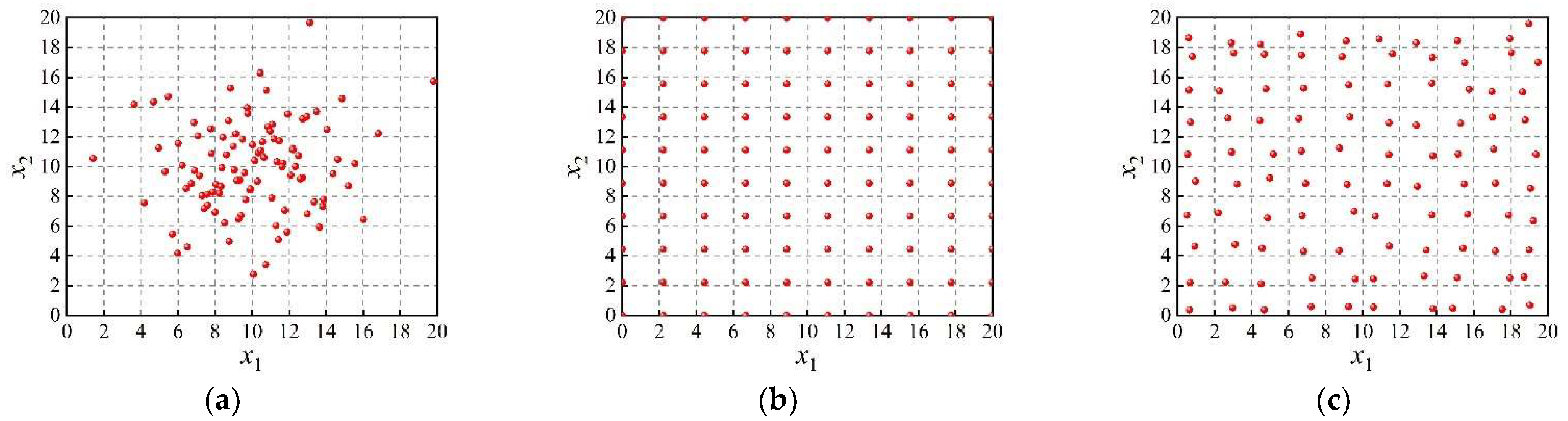
2. Random Moving Quadrilateral Grid Sampling Method

Stratified sampling aims to determine the random value of each variable according to the given variable interval and the number of levels of each variable. Assume that $\Omega$ is a design space with the random variables x and the number of samples is N. The $\Omega$ can be divided into i stratified regions by stratified sampling method, and the space $p_i$ of each stratified region can be described by its probability.

$$p_i=P\left(x_{ij}\in {\Omega }_i\right)\hspace{1em}\hspace{1em}j=1,2,\cdots ,n_i$$

(1)

where i is the number of stratified regions, j is the number of sample points, and $x_{ij}$ is the random sample in the ith stratified region, $j=1,2,\cdots ,n_i$. If $i=1$, the random sampling space will degenerate to the total space.

A vital issue about randomness and uniformity needs to be addressed in the field of initial sample point quality based on the stratified sampling method. Although Latin hypercube sampling (LHS) [41,42] and rectangular grid sampling (RGS) [19] can accurately select the initial sample points in the design space, it is prone to the situation that the sample points are too close or distributed on the boundary, resulting in the reduction of sampling efficiency or the loss of information. Thus, an RMQGS method is proposed based on RGS.

If the dimension of the random variables of the system is m, its value range can be defined as $l_{j^{\prime }}\le x_{j^{\prime }}\le u_{j^{\prime }}$, $j^{\prime }=1,2,\cdots ,m$, and $q_{j^{\prime }}$ represents the level of the j′-dimensional variables. Then, the RMQGS method can be described as follows:

Step 1: The original design space is randomly reduced according to the dimension and level of variables, which is provided as follows:

$${\widehat{u}}_{j^{\prime }}=u_{j^{\prime }}-\alpha \frac{u_{j^{\prime }}-l_{j^{\prime }}}{q_{j^{\prime }}-1},j^{\prime }=1,2,\cdots ,m$$

(2)

where $u_{j^{\prime }}$ and $l_{j^{\prime }}$ are the upper and lower limits of the j′-dimensional variables, and $\alpha$ is random reduction coefficient related to the mean value of design variables, $\alpha =1/\left(\Gamma +rand\right)$, $rand\in \left[0,1\right]$, $\Gamma \in \left[1,+\infty \right)$ is an integer.

Step 2: Grid sampling in a randomly reduced design space, which is provided as follows:

$$x_{j^{\prime }}^{\left(i\right)}=l_{j^{\prime }}+k_{j^{\prime }}^{\left(i\right)}\frac{{\widehat{u}}_{j^{\prime }}-l_{j^{\prime }}}{q_{j^{\prime }}-1}$$

(3)

where $k_{j^{\prime }}^{\left(i\right)}$ is the coefficient related to the levels of the design variable, $k_{j^{\prime }}^{\left(i\right)}=1,2,\cdots ,q_{j^{\prime }}-1$, and i is the number of sample points.

Step 3: A random move is added to the column element $x_i$ and row element $x_j$ of the sample point $x_{ij}$, which is provided as follows:

$$d_{j^{\prime }}=\frac{{\gamma }_{i{j}^{\prime }}}{\lambda }\frac{u_{j^{\prime }}-l_{j^{\prime }}}{q_{j^{\prime }}-1}$$

(4)

where ${\gamma }_{i{j}^{\prime }}$ is the coefficient of motion, which follows a uniform distribution, and $\lambda$ is the coefficient of random moving, $\lambda =\Gamma +rand$.

Step 4: Any two adjacent random moving sample points should satisfy the minimum distance, which is provided as follows:

$$d=\underset{1\le j^{\prime }\le m}{min}\left[\frac{u_{j^{\prime }}-l_{j^{\prime }}}{2\left(q_{j^{\prime }}-1\right)}\left(1-\frac{1}{q_{j^{\prime }}-1}\right)\right]$$

(5)

Step 5: The sample points with random moving in the randomly reduced design space are obtained, which is provided as follows:

$$x_{j^{\prime }}^{\left(i\right)}=l_{j^{\prime }}+k_{j^{\prime }}^{\left(i\right)}\frac{{\widehat{u}}_{j^{\prime }}-l_{j^{\prime }}}{q_{j^{\prime }}-1}+\frac{{\gamma }_{i{j}^{\prime }}}{\lambda }\frac{u_{j^{\prime }}-l_{j^{\prime }}}{q_{j^{\prime }}-1}$$

(6)

3. Reliability Analysis Approach under Multiple Failure Modes

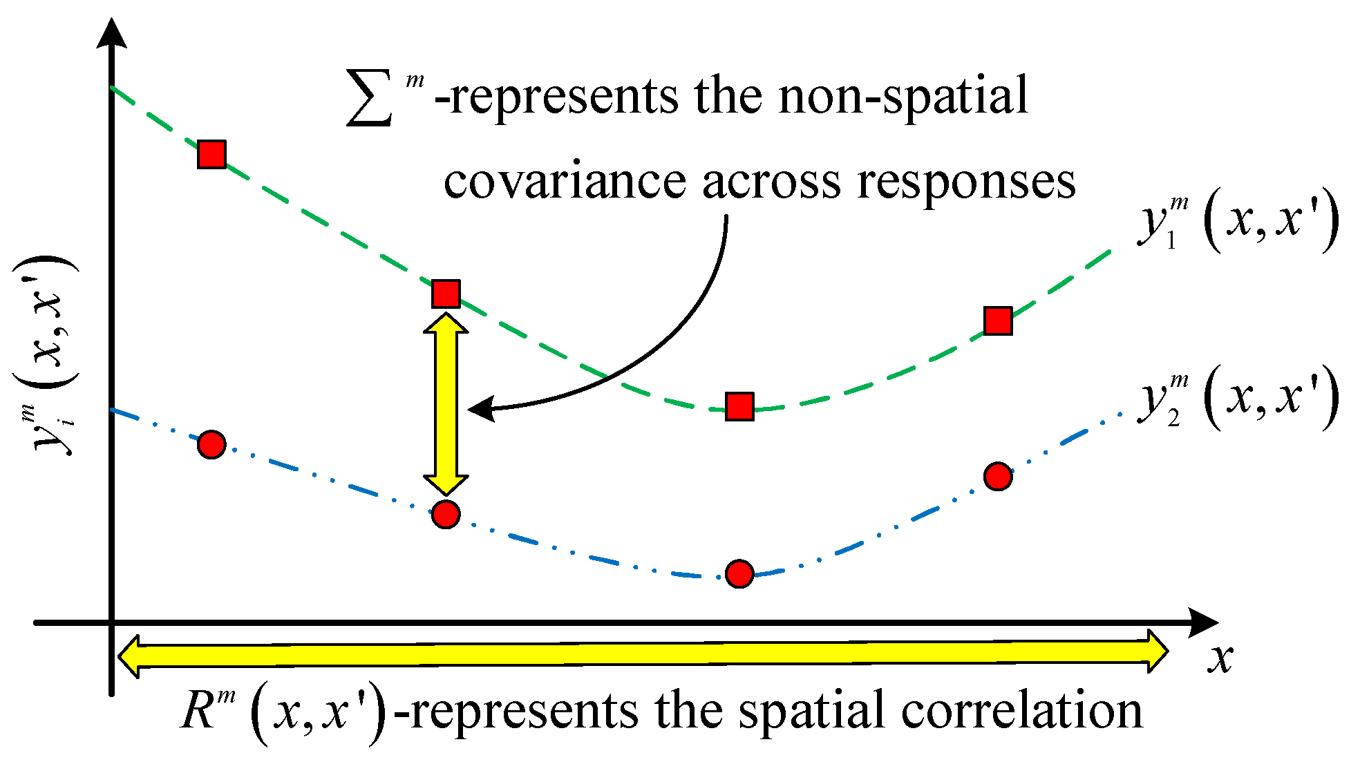
3.1. Adaptive Multiple Response Gaussian Process

Unlike the Kriging model, which regards a single output variable as a Gaussian stochastic process, the MRGP model can treat multi-dimensional output variables $\mathit{y}=\left[y_1,y_2,\cdots ,y_m\right]$ as m-dimensional Gaussian stochastic process with separable covariance functions. Then, the mathematical expression of the MRGP model is described as follows:

$$y^m\left(•,•\right)\sim GP\left({\mathbf{h}}^m\left(•,•\right){\mathbf{B}}^m,{\sum }^m{\mathit{R}}^m\left(\left(•,•\right),\left(•,•\right)\right)\right)$$

(7)

where $GP\left(•,•\right)$ is the Gaussian stochastic process, which is used to construct the global approximate relationship between input variables and output variables, ${\mathbf{h}}^m\left(•,•\right)=\left[h_1^m\left(x,x^{\prime }\right),h_2^m\left(x,x^{\prime }\right),\cdots ,h_n^m\left(x,x^{\prime }\right)\right]$ is the vector of regression models, ${\mathbf{B}}^m=\left[{\beta }_1^m,{\beta }_2^m,\cdots ,{\beta }_n^m\right]$ is the vector of regression coefficients, $R^m\left(•,•\right)$ is a spatial correlation function, which denotes the correlation of spatial location, and ${\sum }^m$ is an unknown covariance matrix, which is the core to deal with the multiple failure models.

Further, to better describe the correlation of multidimensional output response variables, an isotropic Gaussian model is adopted to quantify the correlation of spatial location (Figure 1), which is given as follows:

$$R^m\left(\mathit{x},{\mathit{x}}^{\prime }\right)=\exp \{-{\displaystyle \sum _{k=1}^n{\mathbf{\omega }}_k^m}{\left(x_k^{}-x_k^{\prime }\right)}^2\}$$

(8)

where ${\mathbf{\omega }}_k^m=\left({\omega }_1,{\omega }_2,\cdots ,{\omega }_n\right)$ is the vector of roughness parameters, which represent the rate at which the correlation between multiple failure models decays to zero. The lower values of ${\mathbf{\omega }}_k^m$, the smother MRGP model for the response $y^m\left(•,•\right)$.

For Equation (7), ${\mathbf{B}}^m$ and ${\sum }^m$ are related to the spatial correlation function $R^m\left(•,•\right)$, which is usually expressed by the following equation:

$$\{\begin{array}{l}{\widehat{\mathbf{B}}}^m={\left[{\left({\mathbf{h}}^m\right)}^{\mathrm{T}}{\mathbf{R}}^{-1}{\mathbf{h}}^m\right]}^{-1}{\left({\mathbf{h}}^m\right)}^{\mathrm{T}}{\mathbf{R}}^{-1}\mathbf{Y}\hfill \\ {{\displaystyle \widehat{\sum }}}^m=\frac{1}{p}\left[{\left(\mathbf{Y}-{\mathbf{h}}^m{\mathbf{B}}^m\right)}^{\mathrm{T}}{\mathbf{R}}^{-1}\left(\mathbf{Y}-{\mathbf{h}}^m{\mathbf{B}}^m\right)\right]\hfill \end{array}$$

(9)

where R is the correlation matrix of $R^m\left(\mathit{x},{\mathit{x}}^{\prime }\right)$, Y is the corresponding matrix of response values, and p is the number of sample points.

Due to the solution of roughness parameters ${\mathbf{\omega }}_k^m$ being the key to building the MRGP model, a logarithmic inverse function of the maximum likelihood function $\ln \left[p\left(\mathrm{vec}\left(\mathbf{Y}\right)|{\mathbf{B}}^m,{\sum }^m,{\mathbf{\omega }}_k^m\right)\right]$ is employed.

$$\begin{array}{ll}\ln \left[p\left(\mathrm{vec}\left(\mathbf{Y}\right)|{\mathbf{B}}^m,{\sum }^m,{\mathit{w}}_k^m\right)\right]=& -\frac{mp}{2}\ln \left(2\pi \right)-\frac{p}{2}\ln \left(\left|{\sum }^m\right|\right)-\frac{m}{2}\ln \left(\left|\mathbf{R}\right|\right)\\ & -\frac{1}{2}\mathrm{vec}{\left(\mathbf{Y}-{\mathbf{h}}^m{\mathbf{B}}^m\right)}^{\mathrm{T}}\times {\left({\sum }^m\otimes \mathbf{R}\right)}^{-1}\mathrm{vec}\left(\mathbf{Y}-{\mathbf{h}}^m{\mathbf{B}}^m\right)\end{array}$$

(10)

where $\mathrm{vec}(•)$ represents sorting a matrix by a column vector, and $\otimes$ is the Kronecker product.

The static MRGP model can be built based on Equation (10), which can predict the multidimensional response value $\widehat{\mathbf{y}}\left(x^{*}\right)$ at any unknown point $x^{*}$. The mean and variance of the predicted value can be expressed as follows:

$$\{\begin{array}{l}{\mu }_{\widehat{\mathbf{y}}}\left(x^{*}\right)=h^m\left(x^{*}\right){\mathbf{B}}^{{}^m}+r{\left(x^{*}\right)}^{\mathrm{T}}{\mathbf{R}}^{-1}\left(\mathbf{Y}-{\mathbf{h}}^m{\mathbf{B}}^m\right)\hfill \\ {{\displaystyle \widehat{\sum }}}_{\widehat{\mathbf{y}}}^m=\mathrm{diag}\left(\sum \times \left(\begin{array}{l}\mathbf{1}-r{\left(x^{*}\right)}^{\mathrm{T}}{\mathbf{R}}^{-1}r\left(x^{*}\right)+\\ {\left(h^{{}^m}{\left(x^{*}\right)}^{\mathrm{T}}-{\left({\mathbf{h}}^m\right)}^{\mathrm{T}}{\mathbf{R}}^{-1}r\left(x^{*}\right)\right)}^{\mathrm{T}}\times \\ {\left({\left({\mathbf{h}}^m\right)}^{\mathrm{T}}{\mathbf{R}}^{-1}{\mathbf{h}}^m\right)}^{-1}\left(h^m{\left(x^{*}\right)}^{\mathrm{T}}-{\left({\mathbf{h}}^m\right)}^{\mathrm{T}}{\mathbf{R}}^{-1}r\left(x^{*}\right)\right)\end{array}\right)\right)\hfill \end{array}$$

(11)

where $h^m\left(x^{*}\right)$ is regression model vector at an unknown point $x^{*}$, $r\left(x^{*}\right)$ is the spatial correlation vector between unknown point $x^{*}$ and input sample point, and $\mathrm{diag}(•)$ denotes the diagonal element of the matrix.

The MRGP model can directly build the limit state surface of the structure under multiple failure modes. Although the quality of the initial sample points has been significantly improved by the RMQGS method, the accuracy of the model still cannot meet the requirements due to its limited numbers. Therefore, the adaptability of the MRGP model needs to be enhanced to improve its accuracy and efficiency. Generally, U-function, H-function, and EFF-function are used to search for the best update iteration sample points from the candidate sample points of MC simulation and then update the initial MRGP model until it meets the accuracy conditions. However, the three learning functions have different screening conditions for sample points. If they are used alone, the efficiency is low, and if they are used in combination, the complementary effects are difficult to achieve. To avoid that, two novel learning functions are defined according to the iteration form of the MRGP model.

To increase high-quality sample points, when the number of iterations is odd, the probability value of the U-function is defined as the condition for judging the sign of the maximum possible wrongly predicted response value. The mathematical expression is given as follows:

$${\Theta }_U\left(x\right)=\Phi \left(\left|\frac{{\mu }_{\widehat{y}}\left(x\right)}{{\sigma }_{\widehat{y}}\left(x\right)}\right|\right)$$

(12)

where ${\mu }_{\widehat{y}}\left(x\right)$ and ${\sigma }_{\widehat{y}}\left(x\right)$ denote the predicted mean and standard deviation of the MRGP model, and $\Phi (•)$ is the cumulative distribution function for a standard normally distributed variable. Then, the sample points that need to be updated can be provided as follows:

$${\mathbf{x}}^{\Theta }=\arg \underset{x\in S_{MC}}{\min }{\Theta }_U\left(x\right)$$

(13)

where $S_{MC}$ is the sample repository generated by MC simulation.

When the number of iterations is even, a novel learning function is proposed to screen the sample points closest to the limit state surface, which is expressed as follows:

$${\mathsf{\Upsilon }}_U\left(x\right)=\phi \left(\left|\frac{{\mu }_{\widehat{y}}\left(x\right)}{{\sigma }_{\widehat{y}}\left(x\right)}\right|\right){\displaystyle /}\left|{\mu }_{\widehat{y}}\left(x\right)\right|$$

(14)

where $\phi (•)$ is the probability density function for a standard normally distributed variable. Then, the updated sample points can be given by the following:

$$x^{\mathsf{\Upsilon }}=\arg \underset{x\in S_{MC}}{\max }{\mathsf{\Upsilon }}_U\left(x\right)$$

(15)

Due to the results of Equations (13) and (15) being probability values, the probability evaluation and termination criterion should be made to ensure sample points are updated. The variation coefficient of the estimated failure probability is calculated according to MC simulation, and its expression is provided as follows:

$$\mathrm{Cov}\left({\widehat{P}}_f\right)=\sqrt{\frac{1-{\widehat{P}}_f}{\left(N_{MC}-1\right){\widehat{P}}_f}}$$

(16)

where ${\widehat{P}}_f$ is the estimated failure probability. It is considered that the estimation is unacceptable when $\mathrm{Cov}\left({\widehat{P}}_f\right)\ge 5\%$, and then the sample repository needs to be expanded. Otherwise, it is considered acceptable, and the number of sample points is sufficient.

Further, the termination criterion of the adaptive learning procedure can be expressed as follows:

$$\xi =\frac{N_{MC}-{\displaystyle \sum _{j=1}^{N_{MC}}{\Theta }_U\left(x\right)}}{N_{MC}{\widehat{P}}_f}$$

(17)

where $N_{MC}$ is the number of sample points by MC, when $\xi \le 5\%$, the iteration terminates. Otherwise, some new sample points are added.

3.2. MRGP-SS Based Structure Reliability Analysis

For engineering structures with multiple failure modes, the relationship of each failure mode is mainly in the forms of series, parallel, and series-parallel, etc. Then, their failure probability expression can be provided as follows:

$$P_f=\mathrm{Pr}\left(G_{\chi }\left(\mathit{x}\right),\chi =1,2,\cdots ,m\right)=\{\begin{array}{l}\mathrm{Pr}\left(\underset{\chi =1,2,\cdots ,m}{\min }{G}_{\chi }\left(x\right)\le 0\right),\hspace{1em}\hspace{1em}\hspace{0.17em}\mathrm{series}\\ \mathrm{Pr}\left(\underset{\chi =1,2,\cdots ,m}{\max }{G}_{\chi }\left(x\right)\le 0\right),\hspace{1em}\hspace{1em}\mathrm{parallel}\\ \mathrm{Pr}\left(\underset{\chi =1,2,\cdots ,m}{\mathrm{minmax}}{G}_{\chi }\left(x\right)\le 0\right),\hspace{1em}\mathrm{series-parallel}\end{array}$$

(18)

where $G_{\chi }(•)$ is the $\chi$th limit state equation, which is built using adaptive MRGP, and m is the number of the limit state equation.

The traditional failure probability is mostly based on MC simulation to ensure the accuracy of the results, which is a time-consuming computer-aided program. However, the reliability solution under multiple failure modes belongs to the problem of small failure probability; its efficiency and accuracy have a great impact on the applicability of engineering applications. For these purposes, a novel reliability approach combined with the adaptive MRGP model and SS method is proposed. The principle of SS is to convert the problem of small failure probability into the product of larger conditional probability, if the intermediate events of each sequence satisfy $f_1\supset f_2\supset \cdots \supset f_n=f$, the target failure probability can be expressed as follows:

$$P_F=P\left(F_1\right){\displaystyle \prod _{a=2}^{m}P\left(F_a|F_{a-1}\right)}$$

(19)

where $F=\{G_{\chi }\left(x\right)\le b\}$ is the target failure event, b is the structural response threshold, $F_1$ is the first failure event, $F_a$ is the middle failure event, and $P(F_a|F_{a-1})$ is conduction probability.

In Equation (19), the initial value of conditional probability is usually selected from an interval of $\left[0.1,0.3\right]$. Meanwhile, the value $P\left(F_1\right)$ is determined as follows:

$$P\left(F_1\right)\approx {\tilde{P}}_1=\frac{1}{N}\left[{\displaystyle \sum _{b=1}^N{I}_{F_1}\left({\mathit{x}}_b\right)}\right]$$

(20)

$$\hspace{0.17em}{I}_{F_1}=\{\begin{array}{l}1,\hspace{0.17em}\hspace{0.17em}{\mathit{x}}_b\in F_1\\ 0,\hspace{0.17em}\hspace{0.17em}{\mathit{x}}_b\notin F\end{array}$$

(21)

where $\left\{x_b|b=1,2,\dots ,N\right\}$ is a set of sample points of independent and identically distributed, and $I_{F_1}$ is the indicative function.

Moreover, the Markov chain Monte Carlo simulation is conducted based on an improved Metropolis–Hastings algorithm to produce the condition samples, and the estimated value of conditional probability in a level can be expressed as follows:

$$P\left(F_a|F_{a-1}\right)\approx {\tilde{p}}_a=\frac{1}{N}\left[{\displaystyle \sum _{b=1}^N{I}_{F_{b+1}}({\mathit{x}}_b)}\right]$$

(22)

where ${\tilde{p}}_a$ is the predicted failure probability in a level.

The estimated failure probability of the target failure event is given as follows:

$$\hspace{0.17em}\hspace{0.17em}\hspace{0.17em}\hspace{0.17em}\hspace{0.17em}\hspace{0.17em}\hspace{0.17em}\hspace{0.17em}\hspace{0.17em}\hspace{0.17em}\hspace{0.17em}\hspace{0.17em}{P}_F\approx p_0\left(a-1\right)\frac{N_F\left(a\right)}{N}$$

(23)

where $N_F\left(a\right)$ is the number of sample points, which fall into the failure region in a level.

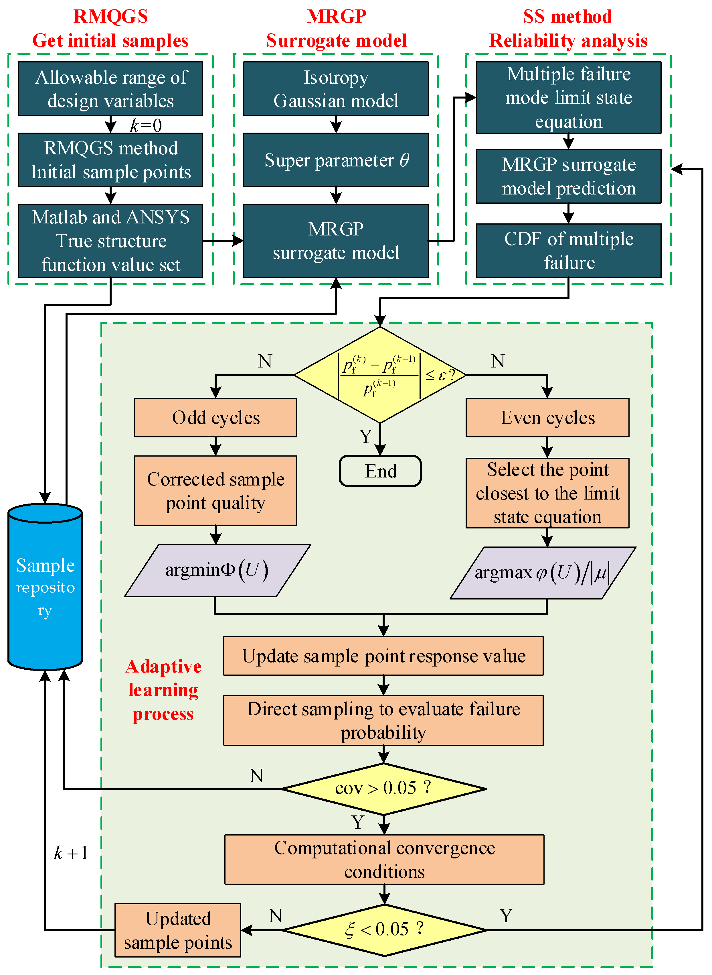
3.3. Summary of the Proposed Method

The flowchart of the proposed method is shown in Figure 2, and it can be summarized as follows:

Stage 1: Obtaining the true response of multiple failure modes using the RMQGS method and Matlab-ANSYS co-simulation.

Step 1: Build a collaborative simulation platform combining Matlab and ANSYS to determine the design variables and design response under multiple failure modes;

Step 2: Generate initial input random variables samples using the RMQGS method;

Step 3: Recording the True structure function value of multiple failure modes based on Step 1 and Step 2.

Stage 2: Building MRGP-SS reliability analysis model.

Step 1: Determine the type of spatial correlation location function of the initial MRGP surrogate model;

Step 2: Estimate the roughness parameters of the MRGP model by employing a logarithmic inverse function of the maximum likelihood function;

Step 3: Build the initial MRGP model using input random variables and their respective true response from the collaborative simulation platform;

Step 4: Build the limit state equation of multiple failure modes based on Step 3;

Step 5: Predict their response by combining the SS method and the limit state equation of multiple failure modes in Step 4;

Step 6: Calculate the CDF of the structure under multiple failures and judge the percentage error between the MC simulation and the MRGP-SS method.

Stage 3: Adaptive MRGP-SS analysis model.

Step 1: Check the accuracy of the MRGP-SS reliability analysis. If the reliability result is accurate enough, the analysis ends. Otherwise, move to stage 3 of the proposed method;

Step 2: If the reliability result is not accurate enough, select a sample with $\mathrm{argmin}\Phi \left(U\right)$ function when the number of iterations is odd, or select a sample with $\mathrm{argmax}\mathsf{\phi }\left(U\right)/\left|\mu \right|$ function when the number of iterations is even;

Step 3: Update the response value and estimate the final failure probability;

Step 4: Check the variance coefficient to ensure the accuracy of the reliability analysis. If its value is less than the given threshold (5%), repeat steps 1–6 of stage 2. Otherwise, check the termination criterion of the adaptive learning procedure; if its value is less than the given threshold (5%), add new samples to the repository for recalculation. Otherwise, repeat steps 1–6 of stage 2;

Step 5: Repeat stages 1–3 until step 1 of stage 3 is accurate enough.

4. Case Studies

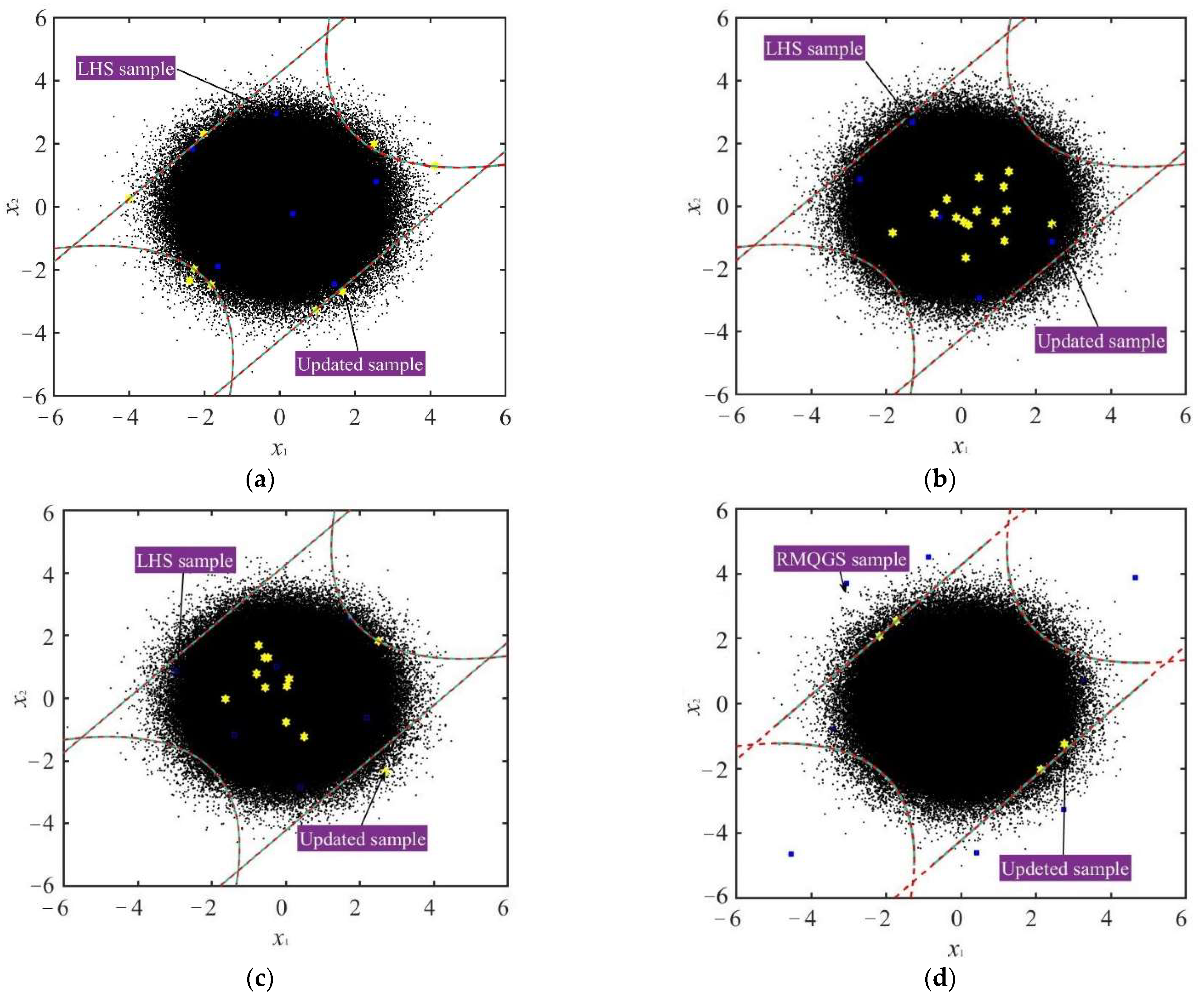
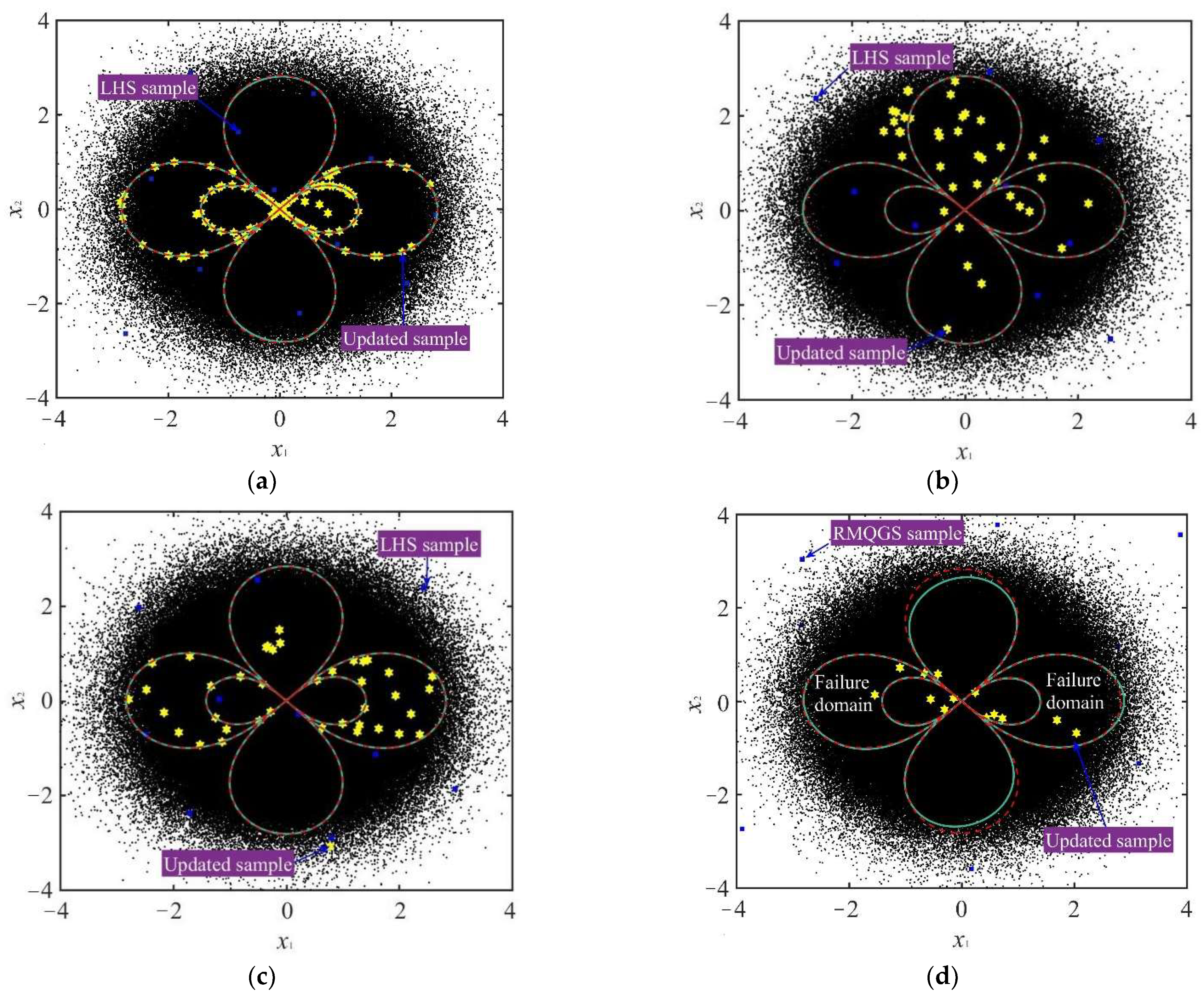
4.1. Validation of RMQGS Method

The methods of LHS and RGS are compared to prove the effectiveness of the proposed RMQGS. Assume that the dimensionless design variables $x_1$ and $x_2$ follow a normal distribution $N\left(10,3^2\right)$, and the range is $\left[0,20\right]$ with 10 levels for each design variable. There are 100 sample points obtained by three methods, as shown in Figure 3.

From Figure 3, the 100 sample points selected by the LHS method have good randomness but poor uniformity, which cannot be distributed in the entire design space. Moreover, there is a phenomenon where the sample points are too concentrated or overlapped, and it is easy to lose the information from the samples. The RGS method makes up for the lack of uniformity of the LHS method to a certain extent and only needs to determine the range of design variables to obtain high-quality samples. However, the randomness of sample points is greater than that of the LHS method, and there are a large number of sample points distributed on the boundary of the design space, resulting in a serious lack of information. The RMQGS method has both the randomness and uniformity of the sample points, which can be uniformly and randomly distributed in each dimension, and the sample information covers the entire sample space. Therefore, the samples selected by the RMQGS method have greater advantages in uniformity and randomness compared with the LHS and RGS methods, and the accuracy of the initial MRGP model can be significantly improved.

4.2. A Numerical Series System Analysis

To verify the applicability and effectiveness of the proposed method, a numerical series system is adopted, and it is compared with a variety of classical combined reliability analysis methods. This numerical series system is composed of four components whose limit state functions are given in Equations (24)–(27) [24]. Among the Equations, x₁ and x₂ follow the standard normal distribution with their independent and identically distributed.

$$G_1\left(x_1,x_2\right)=3+\frac{{\left(x_1-x_2\right)}^2}{10}-\frac{\left(x_1+x_2\right)}{\sqrt{2}}$$

(24)

$$G_2\left(x_1,x_2\right)=3+\frac{{\left(x_1-x_2\right)}^2}{10}+\frac{\left(x_1+x_2\right)}{\sqrt{2}}$$

(25)

$$G_3\left(x_1,x_2\right)=\left(x_1-x_2\right)+\frac{6}{\sqrt{2}}$$

(26)

$$G_4\left(x_1,x_2\right)=\left(x_2-x_1\right)+\frac{6}{\sqrt{2}}$$

(27)

The initial samples are obtained by the RMQGS method according to the range of design variables in Equations (24)–(27), and the true response value of the performance function is solved to build the initial MRGP model, which then calculates the reliability under multiple failure modes and checks its accuracy. Alternate sample points are screened through different active learning functions and convergence criteria, and the best sample points are determined to update the MRGP model, so as to achieve accurate calculation and analysis of reliability under multiple failure modes. In this example, the initial samples of RMQGS are set to 6, and the perfect MRGP model is fitted by the proposed method and its effectiveness is compared by the methods of MRGP + U, MRGP + H, and MRGP + EFF, as shown in Figure 4.

Figure 4 depicts the fitting accuracy of the MRGP model with different active learning functions. In Figure 4, the black dots are MC simulation sample points; the blue dots are initial samples obtained by LHS or RMQGS; the green lines are the fitting curve of the MRGP model; the red lines are the true limit state surface; the yellow dots are updated samples. It can be seen from the figure that the fitting effects of the four methods are almost the same, which is close to the true limit state surface. However, due to the difference between the active learning function and the termination criterion, the number of true performance function calls and the time-consuming are different. Judging from the number of updated samples, the proposed method only needs 4 updated samples to achieve a convergence state, while the methods of MRGP + U, MRGP + H, and MRGP + EFF need 9, 15, and 12 updated samples, respectively. In terms of sample distribution, the initial samples of the RMQGS method have the advantage of randomness and uniformity. It is the basis for ensuring a high-precision initial MRGP model. Then, although the updated samples of the MRGP + U method and the proposed method are close to the limit state surface, the updated samples obtained by the MRGP + U method are concentrated. The updated samples of the MRGP + H method and MRGP + EFF method are far from the limit state surface, and the sample quality is lower than that of the proposed method.

Table 1. Results of example 4.2 with different methods.

Method	Ncalls	${\mathit{P}}_{\mathit{f}}/10^{-3}$	$\mathit{\beta }$	${\mathit{\delta }}_{\mathit{\beta }}/\%$
MC simulation	106	4.52	2.6105	_
Proposed method	10	4.50	2.6121	0.0613
MRGP + U	15	4.45	2.6159	0.2069
MRGP + H	21	4.40	2.6197	0.3524
MRGP + EFF	18	4.35	2.6236	0.5018

shows the reliability comparison results of five different methods under multi-failure models, in which the MC simulation results are used as the accurate solution to verify the reliability accuracy of the other four methods. In Table 1, N_calls denotes the number of calls to the true performance function; P_f denotes the failure probability, $\beta$ denotes the reliability index; ${\delta }_{\beta }$ denotes the percentage error. From Table 1, it is known that the proposed method has high accuracy and efficiency in dealing with the reliability problem of multiple failure modes. Although the reliability results of the proposed method are similar to those of the MRGP + U method, the number of function calls is reduced by 30%. Especially the efficiency of the proposed method is improved by 110% and 44.4%, respectively, compared with the MRGP + H method and the MRGP + EFF method. In general, the proposed method can take into account the accuracy and efficiency of reliability at the same time, and the time-consuming can be significantly saved on the premise of ensuring the solution’s accuracy.

4.3. A Numerical Parallel System Analysis

A parallel system with multiple failure regions is considered to identify the efficiency and accuracy of the proposed method. The reliability problem is defined by Equations (28)–(31) [36].

$$P_f=\mathrm{Pr}\left[G_1\left(\mathit{x}\right)\le 0\cap G_2\left(\mathit{x}\right)\le 0\cap G_3\left(\mathit{x}\right)\le 0\right]$$

(28)

$$G_1\left(x_1,x_2\right)=8x_2{}^2-8x_1{}^2+{\left(x_1{}^2+x_2{}^2\right)}^2$$

(29)

$$G_2\left(x_1,x_2\right)=2x_1{}^2-2x_2{}^2+{\left(x_1{}^2+x_2{}^2\right)}^2$$

(30)

$$G_3\left(x_1,x_2\right)=8x_2{}^2-8x_1{}^2-{\left(x_1{}^2+x_2{}^2\right)}^2$$

(31)

x₁ and x₂ follow the normal distributions with zero mean and unit standard deviation, and the RMQGS method is employed to produce initial samples to build the initial MRGP model. The adaptive MRGP model is then built by the proposed update strategy and termination criterion and compared with the methods of MRGP + U, MRGP + H, and MRGP + EFF, as shown in Figure 5. Finally, the accuracy and efficiency of different methods for the results of reliability analysis are compared in

Table 2. Results of example 4.3 with different methods.

Method	Ncalls	${\mathit{P}}_{\mathit{f}}/10^{-3}$	$\mathit{\beta }$	${\mathit{\delta }}_{\mathit{\beta }}/\%$
MC simulation	106	0.19242	0.8690	_
Proposed method	27	0.19260	0.8684	0.0690
MRGP + U	123	0.19340	0.8654	0.4143
MRGP + H	51	0.19230	0.8695	0.0575
MRGP + EFF	52	0.19180	0.8713	0.2647

.

Figure 5 illustrates the active learning process upon which the MRGP models are built with four different methods. In Figure 5, the initial samples (blue dots) generated by the RMQGS method can cover most of the design space to be efficient, while the samples generated by the LHS method are more concentrated. In general, the MRGP + U method and the proposed method can achieve the sample points added in the vicinity of the limit state, while the updated samples of the MRGP + H method and MRGP + EFF method have high uncertainty. In terms of overall fitting accuracy, the proposed method is lower, but it has high fitting accuracy for the failure domain and requires the least number of sample points, which is beneficial to the reliability analysis.

The results in Table 2 illustrate the efficiency and accuracy of each method, for which 10⁶ samples of an MC simulation population are classified. An MC simulation is performed on the true limit state surface with a population of 10⁶ samples and taken as the reference for the probability of multiple failure models P_f. From Table 2, it is known that the proposed method requires 27 calls to the composite performance function and leads to a relatively good estimation probability of failure. However, the MRGP + U method involves an excessive number of calls (123) to the composite performance function and leads to a relatively poor estimation result. The cause of this imprecision may be that the reliability method cannot effectively be sampled in the failure domain or the quality of sample points is low. Compared with methods of MRGP + H and MRGP + EFF, the computational efficiency of the proposed method is doubled, and the reliability error is lower than that of MRGP + EFF. Although the MRGP + H method has the highest accuracy of reliability in a parallel system, the accuracy of reliability is low in a series system. Overall, numerical examples prove that the proposed method considers both accuracy and efficiency in dealing with the reliability problem under multiple failure modes and can complete the reliability analysis of complex structures efficiently and quickly.

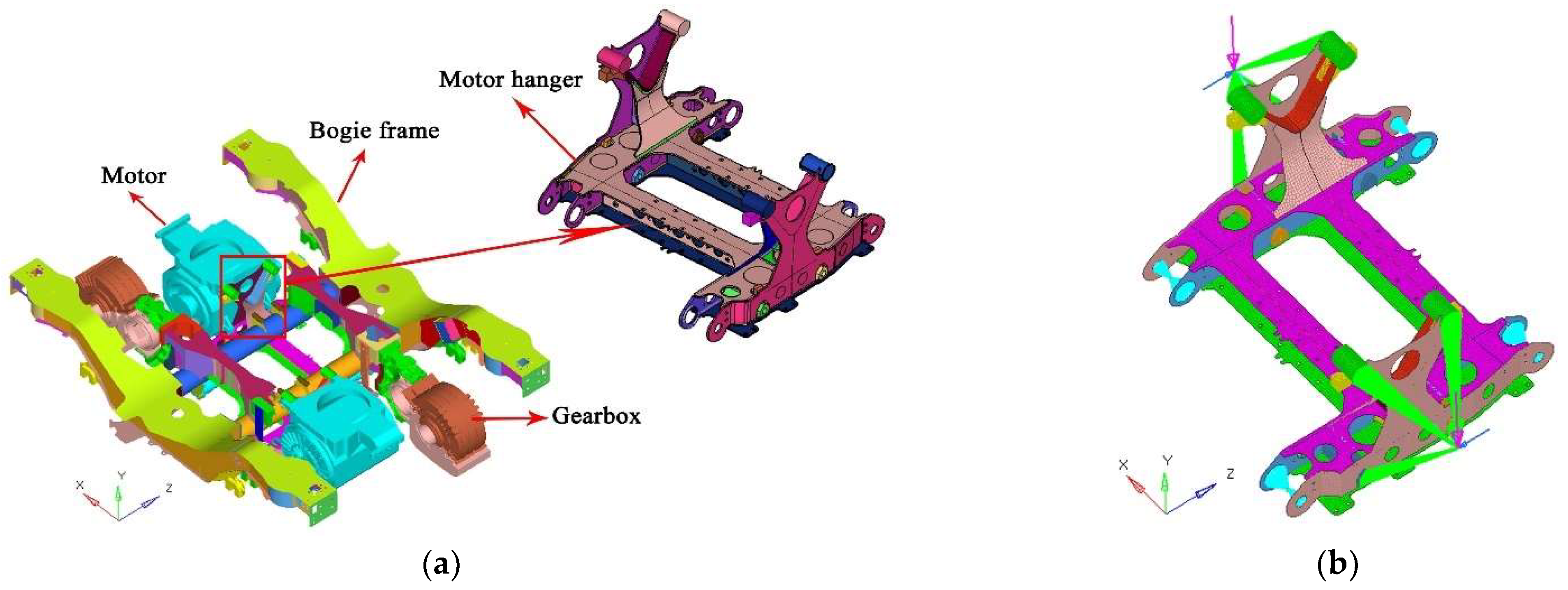
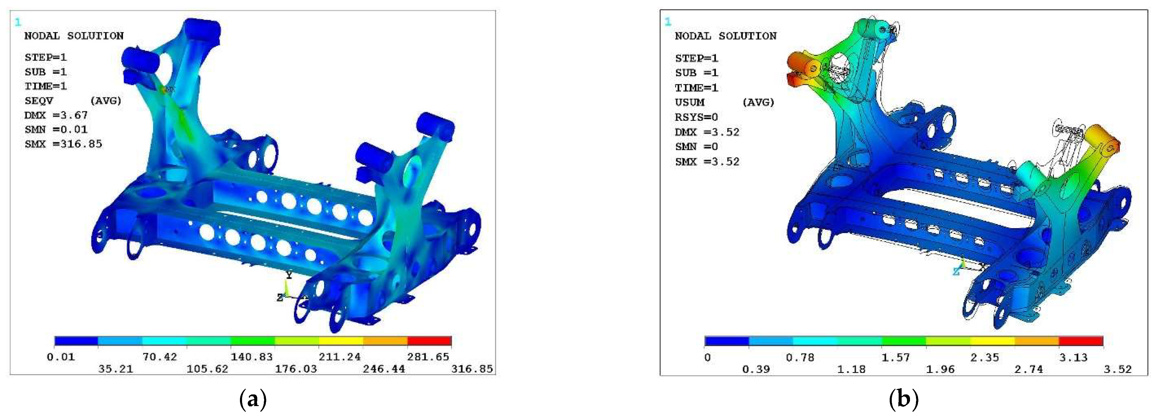
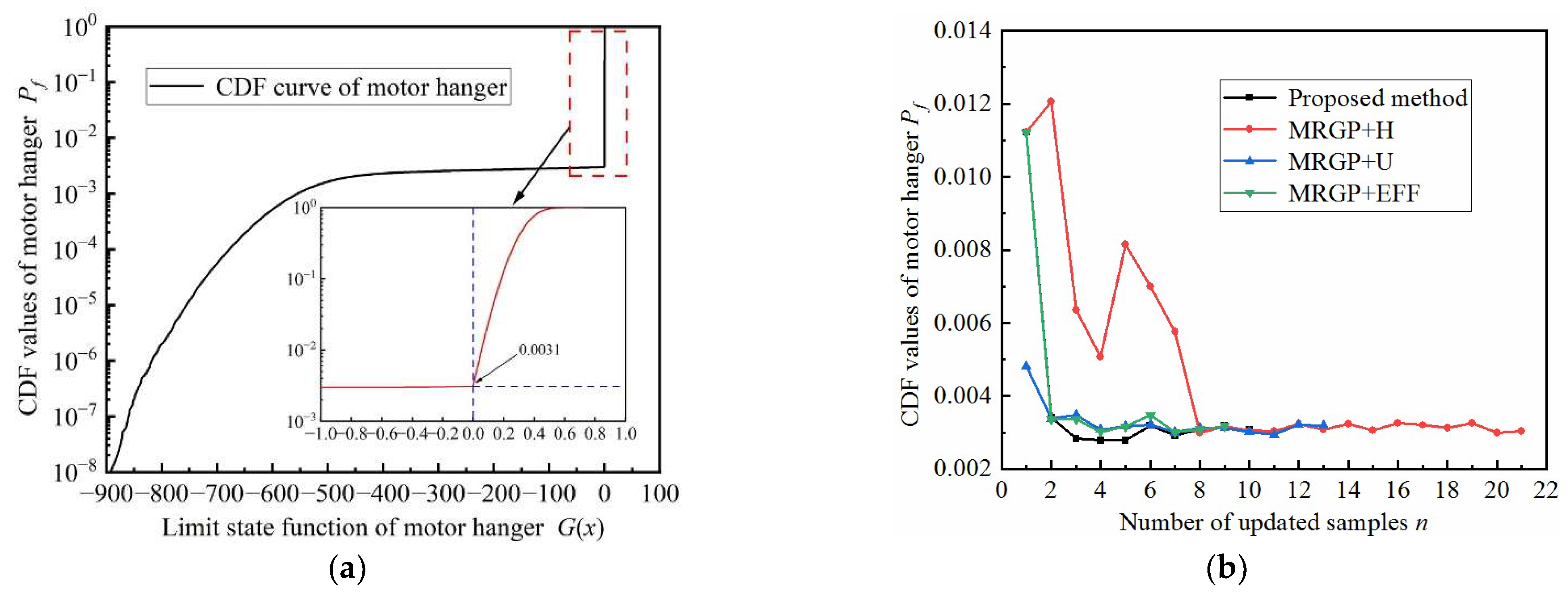
4.4. Motor Hanger Reliability Analysis under Multiple Failure Models

As a key component of the railway vehicle, the function of the motor hanger is to suspend the motor and bear various excitations during train operation. Any form of failure will directly affect the service safety of the train. Therefore, a typical motor hanger is studied to verify the engineering application of the proposed method. Due to the physical model of the motor hanger being difficult to obtain, its failure models can only be simulated by the finite element (FE) simulation method. Then, the FE model of the motor hanger is built according to the characteristics and load cases, as shown in Figure 6. This FE model consists of beam188, shell181, solid185, rigid and rbe3 elements. It is meshed to have 50,879 elements, including 21,766 triangular and quadrilateral shell elements, and 28,973 tetrahedral and hexahedral solid elements. The ANSYS software is employed to perform the structure strength analysis; the stress and displacement nephogram are plotted in Figure 7.

As can be seen from Figure 7, the maximum stress and displacement of the motor hanger are 316.85 MPa and 3.52 mm, respectively, which meet the standard requirements of the maximum allowable stress of 345 MPa and the maximum displacement of 4 mm. However, there are many uncertain factors in the manufacture and operation of the motor hanger, which is easy to make its stress and displacement exceed the allowable range and failure occurs. Therefore, the reliability analysis of the motor hanger is carried out with the help of Matlab and ANSYS collaborative computing platforms, considering the stress and displacement failure modes. Their failure probability limit state equation can be provided as follows:

$$P_f=\mathrm{Pr}\left(\underset{\chi =1,2}{\min }{G}_{\chi }\left(x\right)\le 0\right)=\mathrm{Pr}\{\min \left(\begin{array}{l}345-y_{SEQV}\left(x\right)\le 0\\ 4-y_{USUM}\left(x\right)\le 0\end{array}\right)\}$$

(32)

where x is the random variables, $y_{SEQV}(•)$ is the maximum Mises stress, and $y_{USUM}(•)$ is the maximum displacement.

First, two plate thicknesses and a stochastic load, which have a greater impact on the two failure modes, are selected as random variables. Second, the initial samples are obtained by the RMQGS method, and the ANSYS software is repeatedly called to determine the true response value of the performance function. Finally, the MRGP model is continuously updated iteratively by the proposed method until the reliability accuracy meets the requirements. The reliability analysis results are shown in Figure 8 and

Table 3. Results of example 4.4 with different methods.

Method	Ncalls	${\mathit{P}}_{\mathit{f}}/10^{-3}$	$\mathit{\beta }$	${\mathit{\delta }}_{\mathit{\beta }}/\%$
MC simulation	106	3.2	2.7266	—
Proposed method	18	3.1	2.7370	0.3814
MRGP + U	22	3.1	2.7370	0.3814
MRGP + H	30	2.9	2.7589	1.1846
MRGP + EFF	19	3.0	2.7478	0.7775

.

Figure 8 depicts the CDF curves of the motor hanger with limit state function and updated samples. The reliability of the motor hanger under the two failure models of stress and displacement is 0.9969, i.e., the failure probability is 0.0031. This shows that the motor hanger can maintain high structural performance under the fluctuation of uncertainty factors. It can be seen from Figure 8b that the updated sample sizes of the four methods are 9, 21, 13, and 10, respectively, and the reliability accuracy is the same, indicating that the proposed method can achieve high-precision reliability analysis with the least number of iterations. Table 3 provides the comparative quantification results of the four methods. The accuracy of the proposed method is the same as that of the MRGP + U method, but the efficiency is improved by 18.18%. Moreover, the MRGP + EFF method is slightly lower than the proposed method in both accuracy and efficiency, while the MRGP + H method has a larger difference. In a word, the proposed method has good engineering applicability in dealing with the reliability of the motor hanger with multiple failure modes.

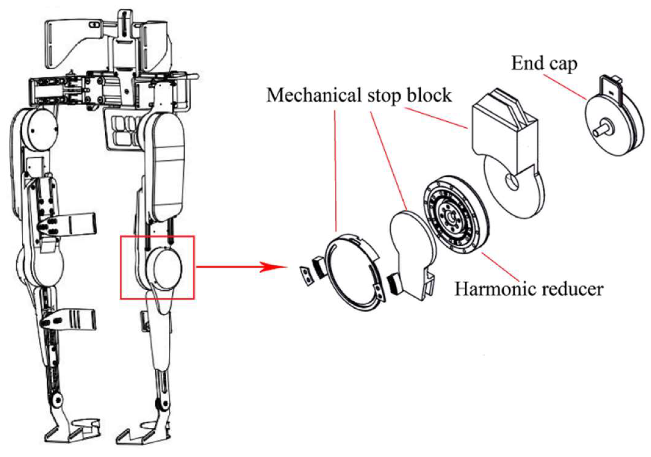
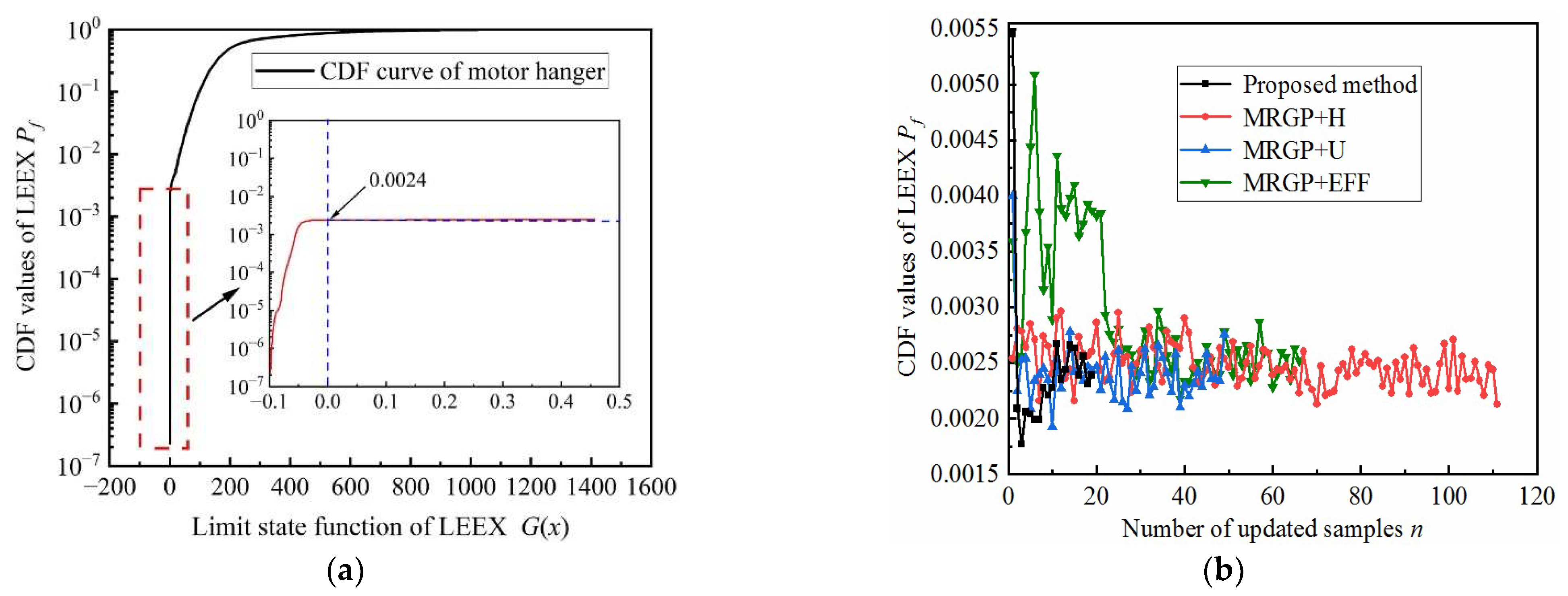
4.5. Reliability Analysis of A Bionic Robot Lower Extremity Exoskeleton (LEEX) under Multiple Failure Models

LEEX is a piece of typical complex equipment, which is mainly composed of a power source, sensing system, control system, driving system, mechanical structure, etc. Due to the uncertainty of the environment, especially the road condition and random shocks, the LEEX will be continuously affected during operation, which will inevitably lead to failure. As the main executive part of the mechanical structure, the harmonic reducer plays a key role in driving LEEX. The harmonic reducer consists of the following four basic components: a wave generator, flexible gear, flexible bearing, and rigid gear. Its main failure modes are tooth surface contact fatigue failure, tooth root bending fatigue failure of flexible gear or rigid gear, and the transmission efficiency failure of harmonic reducer. Therefore, the reliability analysis of LEEX is performed in consideration of the three failure modes of the harmonic reducer. Figure 9 shows a three-dimensional model sketch of the LEEX and the composition of the harmonic reducer.

For the tooth surface contact fatigue failure mode, the limit state function of LEEX can be expressed as follows:

$$G_1\left(\mathit{x}\right)={\sigma }_{Hlim}{Z}_N{Z}_L{Z}_V{Z}_R{Z}_W{Z}_X-{\sigma }_H\sqrt{K{K}_A{K}_V{K}_H}$$

(33)

where ${\sigma }_H$ is contact stress on the tooth surface, ${\sigma }_{Hlim}$ is tooth surface contact fatigue limit, $Z_N$ is life factor, $Z_R$ is roughness coefficient of the tooth surface, $Z_V$ is velocity coefficient, $Z_W$ is working hardening factor, $Z_L$ is lubricant coefficient, $Z_X$ is size factor, K is calculation coefficient; $K_A$ is usage factor, $K_V$ is dynamic load factor, and $K_H$ is load distribution factor along with the direction of tooth width.

For the tooth root bending fatigue failure mode, the limit state function of LEEX can be expressed as follows:

$$G_2\left(\mathit{x}\right)={\sigma }_{Flimj}-{\sigma }_F={\sigma }_{Flim}{Y}_{ST}{Y}_{NT}{Y}_{\delta T}{Y}_{RT}{Y}_X-\frac{1.91\times 10^7{k}_{p}P}{d{n}_{p}nb{m}_n}{Y}_{Fa}{Y}_{Sa}{Y}_{\epsilon }{Y}_{\beta }{K}_A{K}_V{K}_{F\beta }{K}_{F\alpha }$$

(34)

where ${\sigma }_{Flimj}$ is tooth surface bending fatigue strength, ${\sigma }_F$ is bending fatigue stress, ${\sigma }_{Flim}$ is tooth root bending fatigue limit, $Y_{ST}$ is stress correction factor, $Y_{NT}$ life factor, $Y_{\delta T}$ is sensitivity coefficient of relative tooth root fillet, $Y_{RT}$ is coefficient of relative tooth root surface condition, m_n is gear normal modulus, $Y_{Fa}$ is the tooth form factor, $Y_{Sa}$ is stress correction factor, $Y_{\epsilon }$ is contact ratio factor, $Y_{\beta }$ is helix angle coefficient, $K_{F\beta }$ is load distribution factor along with the direction of tooth width, and $K_{F\alpha }$ load distribution factor between teeth.

For the transmission efficiency failure, the limit state function of LEEX can be expressed as follows:

$$G_3\left(\mathit{x}\right)={\eta }_{\mathrm{pm}}-{\eta }_{\min }=\frac{M_2}{\{\left[\mu d_1\frac{7.194\times 10^{-11}Eb\left(K_{bend}{K}_h{d}_m\right)}{m^2{\left(D+d\right)}^3}\right]+\mu d_1\frac{M_2\tan \left({\cos }^{-1}\left(\frac{0.47Z_r}{0.51Z_r+3}\right)+{\tan }^{-1}\left(f\right)\right)}{m\left(Z_r-2\left(h_a^{*}+c^{*}\right)+2\left(3+0.01Z_r\right)-\frac{\delta }{m}\right)}\}i}$$

(35)

where ${\eta }_{\mathrm{pm}}$ is true transmission efficiency, ${\eta }_{\min }$ is minimum transmission efficiency, $M_2$ is output torque, $\mu$ is dynamic resistance coefficient of bearing, E is the modulus of elasticity, $K_{bend}$ is correction coefficient of bending section, $K_h$ is structure coefficient, $d_m$ is flexspline diameter, m is the modulus, $Z_r$ is the number of flexible teeth, $h_a^{*}$ is addendum coefficient, $c^{*}$ is top clearance coefficient, $\delta$ is the thickness of flexible gear ring, and f is friction coefficient of the tooth surface.

The failure probability of LEEX under multiple failure models based on Equations (33)–(35) can be given as follows:

$$P_f=\mathrm{Pr}\left(\underset{\chi =1,2,3}{\max }{G}_{\chi }\left(x\right)\le 0\right)=\mathrm{Pr}\{\max \left(\begin{array}{l}{G}_1\left(x\right)={\sigma }_{Hlimj}-{\sigma }_H\le 0\\ G_2\left(x\right)={\sigma }_{Flimj}-{\sigma }_F\le 0\\ G_3\left(x\right)={\eta }_{\mathrm{pm}}-{\eta }_{\min }\le 0\end{array}\right)\}$$

(36)

To verify the reliability of LEEX under uncertainty factors, five random variables with great influence on three failure modes are selected, and detailed information is presented in

Table 4. Information of random variables.

Symbol	Unit	Distribution	Mean	Mean Square Deviation
$Z_W$	—	Gaussian	1	0.02
K	—	Gaussian	1	0.13
$Y_{ST}$	—	Gaussian	2	0.06
d	mm	Gaussian	24	0.24
$\delta$	mm	Gaussian	4	0.40

.

As mentioned above, the LEEX reliability analysis under multiple failure modes using the proposed method was performed. The proposed RMQGS method is first used to build the initial MRGP model, and then the adaptive MRGP model is built by the update strategy and termination criterion. The LEEX reliability analysis is finally conducted, combined with the SS method, and compared with the MRGP + H, MRGP + H, and MRGP + EFF methods.

Figure 10 illustrates the reliability analysis results of LEEX under multiple failure modes. It can be seen from the results that the reliability of LEEX under the combined effect of tooth surface contact fatigue failure, tooth root bending fatigue failure, and transmission efficiency failure is 0.9976, indicating that the LEEX has high reliability and can resist uncertain changes in the external environment. The solution accuracy of the proposed method is consistent with the MRGP + H and MRGP + EFF methods, but the computational efficiency is improved by 51.53% and 32.76%, respectively, as can be seen in

Table 5. Results of example 4.5 with different methods.

Method	Ncalls	${\mathit{P}}_{\mathit{f}}/10^{-3}$	$\mathit{\beta }$	${\mathit{\delta }}_{\mathit{\beta }}/\%$
MC simulation	106	2.5	2.8070	—
Proposed method	78	2.4	2.8202	0.4681
MRGP + U	99	2.3	2.8338	0.9548
MRGP + H	161	2.4	2.8202	0.4681
MRGP + EFF	116	2.4	2.8202	0.4681

. Although the number of calls and solution accuracy of the MRGP + U method are similar to those of the proposed method, the overall performance is still lower. The reason for the difference in analysis results is that the proposed method can achieve high-precision reliability analysis results with fewer updated samples, as shown in Figure 10b. The proposed method only needs to add 19 updated samples to reach the convergence condition, while the MRGP + H, MRGP + U, and MRGP + EFF methods require 111, 49, and 66, respectively. By comparing the total number of calls, it is found that the proportion of the updated samples in the four methods to the total number of calls is 24.36%, 68.94%, 49.50%, and 56.90%, respectively. This further proves that the initial MRGP built by the proposed method has high accuracy. Above, the analysis shows that the proposed method can achieve the efficient application of multi-failure engineering problems for complex structures under the condition of taking into account the solution efficiency and accuracy.

5. Conclusions

In this paper, a method is proposed to handle the reliability problems under multiple failure models with an adaptive MRGP model. An RMQGS method is first proposed to optimize the uniformity and randomness of initial samples to improve the accuracy of the initial MRGP model. Two novel learning functions for describing the different iterative cycles are presented to build the adaptive MRGP model. The cumulative probability under multiple failure models is estimated by the MRGP-SS method with a few performance function calls. The main conclusions can be summarized as follows:

(1) Compared with LHS and RGS methods, the sample points generated by the proposed RMQGS method can be evenly and randomly distributed in the entire sample space, which effectively avoids the problem of sample points falling on the design space boundary and duplication;

(2) Two numerical examples illustrate the effectiveness of the proposed method in handling multiple failure modes in series and parallel relationships. For the series system, the proposed method improves the efficiency of MRGP + U, MRGP + H, and MRGP + EFF by 30%, 110%, and 44.4%, respectively, under the condition of similar calculation accuracy. For the series system, the proposed method can give both the accuracy and efficiency of calculation compared with MRGP + U, MRGP + H, and MRGP + EFF, and obtain better failure probability estimation with the least number of complex performance function calls;

(3) The reliability analysis of the motor hanger and LEEX under multiple failure modes verifies the engineering application value of the proposed method. The results show that the reliability of the motor hanger under two series failure modes is 0.9969, and the error is only 3.1% compared with the MC simulation method, but the efficiency is significantly improved. The reliability of LEEX under three parallel failure modes is 0.9976, which is the same as the calculation result of MRGP + H and MRGP + EFF, but the efficiency is improved by 51.53% and 32.76%, respectively.

References

1. Bichon, B.J.; McFarland, J.M.; Mahadevan, S. Efficient surrogate models for reliability analysis of systems with multiple failure modes. Reliab. Eng. Syst. Saf. 2011, 96, 1386–1395. [Google Scholar] [CrossRef]
2. Li, G.J.; Lu, Z.Z.; Zhang, X.B.; Zhang, F. A new reliability approach for the fuzzy and random structure based on the uniformly distributed membership level. Int. J. Fuzzy Syst. 2022, 24, 2753–2766. [Google Scholar] [CrossRef]
3. Hasofer, A.; Lind, N. Exact and invariant second-moment code format. J. Eng. Mech. 1974, 100, 111–121. [Google Scholar] [CrossRef]
4. Du, X.P.; Sudjianto, A. First order saddlepoint approximation for reliability analysis. AAIA J. 2004, 42, 1199–1207. [Google Scholar] [CrossRef]
5. Huang, B.Q.; Du, X.P. Probabilistic uncertainty analysis by mean value first order saddlepoint approximation. Reliab. Eng. Syst. Saf. 2008, 93, 325–336. [Google Scholar] [CrossRef]
6. Rosenblueth, E. Two-point estimates in probabilities. Appl. Math. Model. 1981, 5, 329–335. [Google Scholar] [CrossRef]
7. Gorman, M.R. Reliability of Structural Systems; Case Western Reserve University: Cleveland, OH, USA, 1980. [Google Scholar]
8. Yu, S.; Wang, Z. A novel time-variant reliability analysis method based on failure processes decomposition for dynamic uncertain structures. J. Mech. Des. 2018, 140, 051401. [Google Scholar] [CrossRef]
9. Remennikov, A.M.; Murray, M.H.; Kaewunruen, S. Reliability-based conversion of a structural design code for railway prestressed concrete sleepers. Proc. Inst. Mech. Eng. Part F 2012, 226, 155–173. [Google Scholar] [CrossRef]
10. Liu, Y.; Li, T.X.; Liu, K.; Zhang, Y.M. Chatter reliability of turning processing system based on fourth moment method. J. Mech. Eng. 2016, 52, 193–200. (In Chinese) [Google Scholar] [CrossRef]
11. Kaewunruen, S.; Ngamkhanong, C.; Lim, C.H. Damage and failure modes of railway prestressed concrete sleepers with holes/web openings subject to impact loading conditions. Eng. Struct 2018, 176, 840–848. [Google Scholar] [CrossRef] [Green Version]
12. Li, Y.H.; Li, Y.H.; Wang, Y.D.; Wang, J. Structural optimization–based fatigue durability analysis of electric multiple units cowcatcher. Adv. Mech. Eng. 2017, 9, 1–10. [Google Scholar] [CrossRef]
13. Zhi, P.P.; Li, Y.H.; Chen, B.Z.; Shi, S.S. Bounds-based structure reliability analysis of bogie frame under variable load cases. Eng. Fail. Anal. 2020, 114, 104541. [Google Scholar] [CrossRef]
14. Villarrubia, G.; De Paz, J.; Chamoso, P.; Prieta, F. Artificial neural networks used in optimization problems. Neurocomputing 2018, 272, 10–16. [Google Scholar] [CrossRef]
15. Sbarufatti, C.; Corbetta, M.; Giglio, M.; Cadini, F. Adaptive prognosis of lithium-ion batteries based on the combination of particle filters and radial basis function neural networks. J. Power Sources 2017, 344, 128–140. [Google Scholar] [CrossRef]
16. Huang, H.Z.; Wang, H.K.; Li, Y.F.; Zhang, L.L.; Liu, Z.L. Support vector machine based estimation of remaining useful life: Current research status and future trends. J. Mech. Sci. Technol. 2015, 29, 151–163. [Google Scholar] [CrossRef]
17. Marelli, S.; Sudret, B. An active-learning algorithm that combines sparse polynomial chaos expansions and bootstrap for structural reliability analysis. Struct. Saf. 2018, 75, 67–74. [Google Scholar] [CrossRef]
18. Hu, Z.; Mahadevan, S. Global sensitivity analysis-enhanced surrogate (GSAS) modeling for reliability analysis. Struct. Multidiscip. Optim. 2016, 53, 501–521. [Google Scholar] [CrossRef]
19. Gao, Y.H.; Wang, X.C. An effective warpage optimization method in injectionmolding based on the kriging model. Int. J. Adv. Manuf. Tech. 2008, 37, 953–960. [Google Scholar] [CrossRef]
20. Ma, Y.Z.; Li, H.S.; Yao, W.X. Reliability-based design optimization using a generalized subset simulation method and posterior approximation. Eng. Optim. 2018, 50, 733–748. [Google Scholar] [CrossRef]
21. Huang, D.; Allen, T.T.; Notz, W.I.; Zeng, N. Global optimization of stochastic black-box systems via sequential kriging meta-models. J. Glob. Optim. 2012, 54, 431. [Google Scholar] [CrossRef] [Green Version]
22. Li, Z.; Ruan, S.; Gu, J.F.; Wang, X.Y.; Shen, C.Y. Investigation on parallel algorithms in efficient global optimization based on multiple points infill criterion and domain decomposition. Struct. Multidiscip. Optim. 2016, 54, 747–773. [Google Scholar] [CrossRef]
23. Bichon, B.J.; Eldred, M.S.; Swiler, L.P.; Mahadevan, S.; Mcfarland, J.M. Efficient global reliability analysis for nonlinear implicit performance functions. AIAA J. 2008, 46, 2459–2468. [Google Scholar] [CrossRef]
24. Echard, B.; Gayton, N.; Lemaire, M. AK-MCS: An active learning reliability method combining Kriging and Monte Carlo simulation. Struct. Saf. 2011, 33, 145–154. [Google Scholar] [CrossRef]
25. Zhao, D.Y.; Yu, S.; Wang, Z. A box moments approach for the time-variant hybrid reliability assessment. Struct. Multidiscip. Optim. 2021, 64, 4045–4063. [Google Scholar] [CrossRef]
26. Sun, Z.; Wang, J.; Li, R.; Tong, C. LIF: A new Kriging based learning function and its application to structural reliability analysis. Reliab. Eng. Syst. Saf. 2017, 157, 152–165. [Google Scholar] [CrossRef]
27. Tee, K.F.; Ebenuwa, A.U. Combination of line sampling and important sampling for reliability assessment of buried pipelines. Proc. Inst. Mech. Eng. Part O 2018, 233, 1748006X1876498. [Google Scholar] [CrossRef]
28. Yuan, X.K.; Zheng, Z.X.; Zhang, B.Q. Augmented line sampling for approximation of failure probability function in reliability-based analysis. Appl. Math. Model. 2020, 80, 895–910. [Google Scholar] [CrossRef]
29. Jinsuo, N.; Ellingwood, B.R. Directional methods for structural reliability analysis. Struct. Saf. 2000, 22, 233–249. [Google Scholar] [CrossRef]
30. Li, H.S.; Xia, S.; Luo, D.M. A probabilistic analysis for pin joint bearing strength in composite laminates using Subset Simulation. Compos. Part B-Eng. 2014, 56, 780–789. [Google Scholar] [CrossRef]
31. Huang, X.X.; Chen, J.Q.; Zhu, H.P. Assessing small failure probabilities by AK-SS: An active learning method combining kriging and subset simulation. Struct. Saf. 2016, 59, 86–95. [Google Scholar] [CrossRef]
32. Ditlevsen, O. Narrow reliability bounds for structural system. J. Struct. Mech. 1979, 7, 453–472. [Google Scholar] [CrossRef]
33. Zhi, P.P.; Wang, Y.D.; Wang, Z.L.; Li, Y.H.; Zhang, M. IDEPSO-SS based reliability analysis of bogie frame under multiple load cases. China Railw. Sci. 2021, 42, 134–143. (In Chinese) [Google Scholar]
34. Zhang, Y.C. High-order reliability bounds for series systems and application to structural systems. Comput. Struct. 1993, 46, 381–386. [Google Scholar] [CrossRef]
35. Song, J.H.; Der Kiureghian, A. Bounds on system reliability by linear programming. J. Eng. Mech. 2003, 129, 627–636. [Google Scholar] [CrossRef]
36. Fauriat, W.; Gayton, N. AK-SYS: An adaptation of the AK-MCS method for system reliability. Reliab. Eng. Syst. Saf. 2014, 123, 137–144. [Google Scholar] [CrossRef]
37. Yang, X.F.; Mi, C.Y.; Deng, D.Y.; Liu, Y.S. A system reliability analysis method combining active learning Kriging model with adaptive size of candidate points. Struct. Multidiscip. Optim. 2019, 60, 137–150. [Google Scholar] [CrossRef]
38. Yun, W.Y.; Lu, Z.Z.; Zhou, Y.C.; Jiang, X. AK-SYSi: An improved adaptive Kriging model for system reliability analysis with multiple failure modes by a refined U learning function. Struct. Multidiscip. Optim. 2019, 59, 263–278. [Google Scholar] [CrossRef]
39. Arendt, P.D.; Apley, D.W.; Chen, W. Improving identifiability in model calibration using multiple responses. J. Mech. Des. 2012, 134, 100909. [Google Scholar] [CrossRef]
40. Wei, P.; Liu, F.; Tang, C. Reliability and reliability-based importance analysis of structural systems using multiple response Gaussian process model. Reliab. Eng. Syst. Saf. 2018, 175, 183–195. [Google Scholar] [CrossRef]
41. Shu, Z.; Jirutitijaroen, P. Latin hypercube sampling techniques for power systems reliability analysis with renewable energy sources. IEEE Trans. Power Syst. 2011, 26, 2066–2073. [Google Scholar] [CrossRef]
42. Xiao, N.C.; Yuan, K.; Zhan, H.Y. System reliability analysis based on dependent Kriging predictions and parallel learning strategy. Reliab. Eng. Syst. Saf. 2022, 218, 108083. [Google Scholar] [CrossRef]
Figure 1. Principle of the MRGP model in dealing with the correlation of multiple failure modes.
Applsci 12 08961 g001
Figure 2. Flowchart of the proposed method.
Applsci 12 08961 g002
Figure 3. Scatter plot of different sampling methods. (a) LHS; (b) RGS; (c) RMQGS.
Applsci 12 08961 g003
Figure 4. MRGP models and its samples distribution for the series system. (a) MRGP + U; (b) MRGP + H; (c) MRGP + EFF; (d) Proposed method.
Applsci 12 08961 g004
Figure 5. MRGP models and its samples distribution for the parallel system. (a) MRGP + U; (b) MRGP + H; (c) MRGP + EFF; (d) Proposed method.
Applsci 12 08961 g005
Figure 6. Structure characteristic and FE model of the motor hanger. (a) Geometric model of the motor hanger; (b) FE model of the motor hanger.
Applsci 12 08961 g006
Figure 7. Static strength analysis of motor hanger. (a) Stress nephogram; (b) Displacement nephogram.
Applsci 12 08961 g007
Figure 8. Reliability analysis results of the motor hanger under multiple failure modes. (a) CDF curve of the motor hanger; (b) Iterative curve of CDF.
Applsci 12 08961 g008
Figure 9. Model sketch of LEEX robot and harmonic reducer.
Applsci 12 08961 g009
Figure 10. Reliability analysis results of LEEX under multiple failure modes. (a) CDF curve of IEEX; (b) Iterative curve of CDF.
Applsci 12 08961 g010