On the Efficacy of Turbulence Modelling for Sloshing

Abstract

As part of a wider project to understand the applicability of utilising slosh-based damping for wing-like structures, simulations of partially filled tanks subjected to harmonically oscillating and vertical motion are presented. The Volume of Fluid modelling approach is used to capture the air–water interface and different turbulence models based on the Reynolds Averaged Navier–Stokes equations employed. No-model simulations are also conducted to demonstrate the efficacy of using turbulence models in the simulation of sloshing flows. Accuracy of the models is assessed by comparing with recent well-validated experimental data in terms of the damping effect of the sloshing. A wide range of excitation amplitudes are considered in the study to demonstrate the effectiveness of different turbulence models in representing the flow feature of weak and very violent sloshing. The results show that standard turbulence models can produce an excessive dissipation, especially at the interface, leading to inaccuracies in the estimation of sloshing dynamics of the violent sloshing. This issue is absent in the no-model simulations, and better results are obtained for all tested sloshing conditions, suggesting approaches to mitigate this interfacial dissipation within RANS-based modelling is an important consideration for future direction.

1. Introduction

The sloshing of liquid in a partially filled tank is seen in many engineering applications, for example, sloshing of liquefied natural gas (LNG) inside tanks during transportation can be problematic, with excessive and dynamic loads on the walls [1,2,3]. In other applications, liquid sloshing can be used as a positive phenomenon in order to provide additional mechanical damping to a system. A tuned liquid damper (TLD) is such an example and exploits sloshing to reduce the response of tall structures to external aerodynamic effects in order to improve serviceability [4]. In aviation applications, Merten and Stephenson [5] and, very recently, Constantin et al. [6] demonstrated that fuel sloshing inside aircraft wings has an appreciable damping effect. Constantin et al. [7] showed different linear damping response patterns with a scope to alleviate the gust loads on aircraft. For the damping to be effective, the sloshing load should be out of phase with the external force [8,9]. Additionally, at natural frequencies, sloshing loads can be excessive, leading to structural damage [1,2,3]. Therefore, a reliable prediction of the sloshing dynamics is essential for the design and operation of the system subjected to sloshing influence. This work forms part of the wider EU Horizon 2020 SLOWD (SLOshing Wing Dynamics) project and investigates the physics of fuel sloshing in the context of wing-like structures in order to build reliable experimental, numerical and theoretical modelling frameworks that inform future wing designs and reduce design conservatism [10,11].

Experimental approaches to understand sloshing dynamics have been widely used, for example, several experimental works were conducted by Fujino et al. [12,13], Molin and Remy [14], Cavalagli et al. [15] to study and characterise tuned mass dampers. Hu et al. [16], Yan et al. [17] studied the impact load of breaking waves on coastal structures. The survivability of a moored floating production storage and offloading model was assessed by Hu et al. [18]. The coupled rolling motion of a ship with a tank sloshing was studied by Lee et al. [19] and Huang et al. [8], showing a rolling damping effect when the tank’s dimension and filling level are carefully chosen. Constantin et al. [7] and Martinez-Carrascal and González-Gutiérrez [20] investigated the transient damping response of single degree-of-freedom system to different excitation amplitude and filling levels. They showed a high damping response at the start of the transition, which is important to mitigate the aircraft gust loads. Mimicking an aircraft wing, a scaled cantilever beam with partially filled tanks at the tip was developed by Titurus et al. [21] to study the damping effect of different filling levels. The experimental measurements can be considered the most reliable approach to study the fluid dynamics of the problem, albeit this is limited by the number and the type of variables that can be realistically quantified. Additionally, for the sloshing problem, scaling from experimental models to full-scale implementation is not trivial [22,23], and this is especially true in an industrial context.

Computational fluid dynamics (CFD) can provide a comprehensive representation of flow features that are usually difficult or impossible to obtain experimentally. Additionally, with appropriate modelling approaches and computational resources, CFD can be used to study full-scale problems. Smoothed Particle Hydrodynamics (SPH) has been used for the modelling of free surface flows, such as sloshing and waves [7,24,25,26,27,28]. Level set methods have also been used to define the free surface [29,30] in sloshing problems. Finite-volume discretisation combined with the Volume of Fluid (VoF) method is available in many commercial and open-source CFD solvers and presents a common methodological approach to solving sloshing-type problems. Higuera et al. [31], Ransley [32] and Hu et al. [18] used VoF to study waves and their interactions with fixed and floating structures, with a good agreement with experimental data, and the successful use of VoF for sloshing problems was demonstrated in [33,34,35,36,37,38,39,40].

High-resolution simulations that capture the flow physics down to the Kolmogorov length scale, i.e., direct numerical simulation, can be prohibitively expensive in computational terms. Therefore, a less expensive simulation can be conducted via turbulence modelling. Wright et al. [40] produced a very accurate representation of the dynamics of violent vertical sloshing via large eddy simulation (LES). However, full-scale studies via LES can also be very expensive, especially for wall-bounded flows where the boundary layer has to be resolved [41]. Reynolds-averaged Navier–Stokes simulation (RANS) represents a potential and less computationally demanding alternative. However, there is a lack of consensus regarding whether commonly employed turbulence models should be used for free surface problems, while sloshing simulation without a turbulence model has been widely used with good accuracy [29,42,43,44]. Lee et al. [45], Chintalapati and Kirk [46] illustrated that the sloshing load is insensitive to the use of turbulence modelling. Craig et al. [47] also showed that RANS simulation using k-$\omega$ was less accurate than its no-model flow counterpart. Recently, Cai et al. [48] compared between different free surface capturing approaches (VoF, SPH, ALE) and they also compared the prediction accuracy of unsteady k-$ϵ$, LES-WALE and DES, and no-model. They found that the no-model and the LES model provided the best correlation to the experimental results, which is in line with our general findings but is not a complete answer as we know that the no-model approach is sub-optimal for complex sloshing flows while a full LES simulation is often excessively computationally intensive, especially in an industrial context. Kamath et al. [30] demonstrated that the RANS model can suffer an over-production of turbulence at the interface due to the large velocity gradient that can be evident. Mayer and Madsen [49] and Larsen and Fuhrman [50] proved that most two-equation closed problems suffer an unstable exponential growth of turbulent kinetic energy. To overcome this issue, several treatments for the models near the interface are proposed [30,49,50].

Conversely, several studies have shown the importance of turbulence models in the simulation of free surface flows. Realising the lack of consensus on the importance of turbulence modelling in sloshing simulations, [51,52] assumed sloshing is a turbulent phenomenon, and standard turbulence models were used. Rhee [53] showed that a lack of turbulence modelling can lead to non-physical irregularities and instabilities in the no-model solution. The sensitivity study of Godderidge et al. [54] also suggested that a laminar assumption is not appropriate in a sloshing flow and that turbulence modelling has to be employed to obtain accurate representation. Additionally, Liu et al. [55] compared between RANS, LES and very large eddy simulations and concluded that an adequate energy dissipation via turbulence modelling is key in the predictions of plunging wave breaking.

Kamath et al. [30] argued that k-$\omega$ is more suitable and stable for the simulation of unsteady two-phase flow due to the linear relationship between the turbulent kinetic energy and the specific turbulent dissipation rate, while a reliable simulation of rolling response of a ship with an internal tank was conducted with k-$\omega$ SST [8]. Hu and Kamra [56] computed the impact pressure of sloshing using the standard k-$ϵ$, realizable k-$ϵ$ and Wilcox k-$\omega$ models, and they found that predictions of standard k-$ϵ$ and Wilcox k-$\omega$ models were very close and accurate. Tahmasebi et al. [57] tested eight turbulence models for simulating transverse sloshing in a rectangular tank. They found that RNG k-$ϵ$ and k-$\omega$ SST performed best in predicting the free surface behaviour. Thus, a proper selection of the turbulence model is clearly key for providing an accurate representation of fluid-sloshing dynamics. Brown et al. [58] evaluated a library of turbulence models in predicting different characteristics of spilling and plunging wave breakers. The results were not particularly conclusive in that the models which performed well for plunging breakers were often inaccurate when capturing the dynamics of spilling breakers. While no-model simulations produced acceptable results, they found that, in general, using turbulent models can improve the accuracy and efficiency relative to the no-model cases. Therefore, it is believed that the predictability of turbulence closure models for multi-phase flow is case dependent, depending largely on the surface-breaking characteristics.

In this work, we investigate the accuracy of turbulence models in predicting the forces and associated dissipated energy of fluid sloshing in a vertically oscillating tank. This is performed by comparing with validated and unique experimental data obtained within the SLOWD project [59]. As shown in the coming sections, relying on a single case, as was done in Liu et al. [55], Hu and Kamra [56], Tahmasebi et al. [57], to compare between simulation setups can be misleading. Whereby a setup that works well in one case can fail for another apparently similar setup. Therefore, we aim to improve understanding of how to characterise when different models are the most appropriate by providing a comparison between different turbulence modelling using the VoF approach for a number of modes of sloshing dynamics defined according to their Froude number (Fr). The range of Fr numbers considered here corresponds to different sloshing dynamics ranging from a weak sloshing motion through to a very turbulent and violent sloshing. This allows for a more reliable and conclusive comparison between the models and provides a basis to make a decision as when to apply each within a complex sloshing simulation involving multiple regimes simultaneously.

This paper is organised as follows: a problem description and definition of the formulations to compute the dissipation is presented in Section 2, followed by the numerical setup in Section 3. Then, results and discussion of the accuracy of the numerical simulations are presented in Section 4. A summary of conclusions and future works are presented in Section 5.

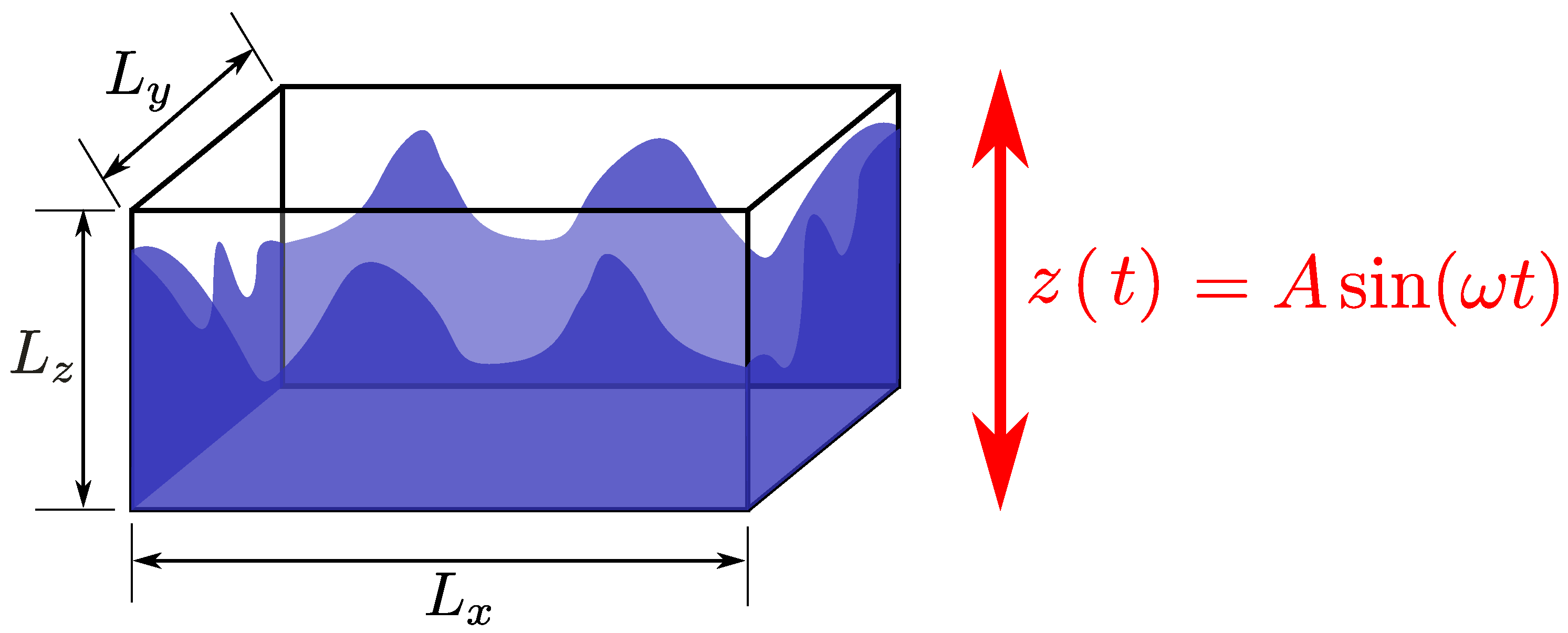
2. Problem Description

Simulations of a vertically oscillating tank with a single harmonic motion are presented. The simulations replicate the physical experiment of Constantin et al. [59], which is illustrated in the schematic diagram shown in Figure 1. This consists of a closed cuboid tank, half-filled with water, with the dimensions $L_x=10$ cm, $L_y=3$ cm and $L_z=5$ cm, where, z represents the vertical direction. The tank is forced to oscillate vertically with a constant amplitude, A, and a frequency, f, and hence the displacement of the tank is expressed with a sinusoidal relationship as

$$z=A\sin \left(\omega t\right),$$

(1)

where, z is the displacement of the tank from the origin, $\omega =2\pi f$, and t is the time. As can be seen in Equation (1), for a given tank, the dominant parameters determining the sloshing damping effect are the amplitude and the frequency of the oscillation. These two parameters are combined as a non-dimensional Froude number $Fr$, that represents the ratio between the inertial and the gravitational forces, i.e.,

$$Fr=\sqrt{\frac{A{\omega }^2}{g}}$$

(2)

In their results, Constantin et al. [59] detailed the measurements of damping forces and an analysis of the recorded sloshing dissipation energy. This renders the case a good benchmark for testing modelling simulation setups and different turbulence models. The work presented in [59] is part of an active research project, and the authors provided a newer version of the experimental data than used in [59] that has less uncertainty, these are used within this work.

The tests are conducted for a range of $Fr=0.7$ to $Fr=1.85$ and are compared directly against the experimental data. The Fr number is changed by keeping the frequency constant at $\omega =52.15$, while varying the amplitude between $A=1.72$ mm to $12.46$ mm. This range covers two types of sloshing regimes, $R_1$ and $R_2$, as referred to in [7,59]. In the $R_1$ regime, sloshing is turbulent and associated with high damping. This is mainly caused by the liquid impacting the upper and lower walls that results from the high excitation. In the lower excitation $R_2$ regime, damping is seemingly caused by typical sloshing modes without surface breaking [59].

Comparison with experiment is based on the damping force induced by the sloshing and the associated dissipated energy. Energy dissipation is quantified via hysteresis loop analysis of the hydrodynamic forces acting on the tank walls. Throughout the simulations, the vertical forces on the inner tank walls are recorded at every time step. The recorded forces are the sum of the pressure force acting on the horizontal walls, $F_p$, and the sum of the viscous forces acting on the vertical walls, $F_{\nu }$. The total force exerted on the tank walls in the direction of the motion can be expressed as [7,15]

$$F_T=F_p+F_{\nu }.$$

(3)

The total force consists of the static loading of the water in the tank, inertia of the water as the tank accelerates and decelerates, and the damping effect of the fluid sloshing inside the tank, this can be expressed as

$$F_T=m_{w}g+m_w\ddot{z}+F_s,$$

(4)

where $m_w$ is the mass of the water (i.e., 75 g), g the gravitational acceleration and $F_s$ is the damping force of the sloshing. The water mass and tank acceleration are predetermined, and the damping force can be computed as a function of time.

Sloshing is an unsteady process and the damping forces can vary from cycle to cycle, especially during turbulent sloshing. All presented simulations start with stationary and undisturbed liquid, which go through a transition period before hitting a statistically steady state. The simulations run for a total time of 20 s, this corresponds to 166 cycles (the excitation frequency is $\omega =52.15$ rad/s and the period is $T_p=0.12$ s). It is observed that, for the range of $Fr>1$, the first 30 cycles are sufficient to pass the transition period, while for the low $Fr$ the transition time is longer, around 60 cycles. In order to quantify the mean dissipated energy, the damping force is phase-averaged after the transition period according to

$${\overline{F}}_s\left(t\right)=\frac{1}{N}\sum _{n=1}^N{F}_s(T_p\times n+t),$$

(5)

where $T_p$ is the period of one cycle, n is the cycle number, and N is the total number of cycles considered in the averaging. ${\overline{F}}_s\left(t\right)$ is the phase average force function of time for one cycle.

The induced dissipation energy can be estimated as the work required to displace the tank against the sloshing force [7,15]. In the case of the sinusoidal oscillation of the tank, the dissipated energy is equivalent to the enclosed area of the force–displacement hysteresis loop and can be expressed as

$$e_s=\int {\overline{F}}_s\left(t\right)dz.$$

(6)

This integration is estimated by the trapezoidal rule. Non-dimensional energy dissipation is used to compare with published experimental results, which were obtained by normalising $e_s$ with respect to half of the maximum kinetic energy of the liquid according to

$$E_s=\frac{e_s}{m_w{\omega }^2{A}^2}.$$

(7)

3. Methodology

The multiphase VoF fluid solver interFoam, from the OpenFOAM v8 [60] code base is employed to simulate a vertically oscillated sloshing tank with harmonic motion. This solves the incompressible Navier–Stokes equations expressed as an arbitrary moving volume to account for moving boundaries [61,62]. These are in the form

$$\nabla ·\mathit{U}=0,$$

(8)

and

$$\frac{\partial {\rho }_f\mathit{U}}{\partial t}+\nabla ·[\mathit{U}·{\rho }_f(\mathit{U}-{\mathit{U}}_{\mathit{s}})]=-\nabla p+\nabla ·\left[(\mu +{\mu }_t)\nabla \mathit{U})\right]+{\mathit{s}}_{\mathsf{\varphi }},$$

(9)

where ${\rho }_f$ is the fluid density, t is the time, ${\mathit{U}}_{\mathit{s}}$ is the velocity of the surface S (i.e., the grid velocity), $\mu$ is the dynamic viscosity of the fluid, p is the fluid pressure and ${\mathit{s}}_{\mathsf{\varphi }}$ is a source term that includes both surface tension and gravity. The VoF method is used to capture the liquid–gas interface. In this approach, the density and viscosity are determined locally as a ratio of the occupying fluid:

$$\begin{array}{c}\hfill {\rho }_f=(1-\alpha ){\rho }_g+\alpha {\rho }_l,\\ \hfill \mu =(1-\alpha ){\mu }_g+\alpha {\mu }_l\end{array}$$

(10)

where the subscripts g and l refer to the properties of the gas and liquid (here, properties are for air and water). $\alpha$ is the volume fraction of the liquid. The interface is constructed with the Multidimensional Universal Limiter for Explicit Solution (MULES) scheme, and artificial interface compressibility is employed to prevent excessive numerical diffusion of the phase fraction field [63]. In our work herein, the extent of the interface compression is set conservatively, such that spurious deformation is prevented, while still being effective in reducing interface numerical diffusion. The OpenFOAM keyword cAlpha controls the extent of this compression and is set to the widely adopted value of 1 in all simulations presented [37].

The turbulent viscosity ${\mu }_t$, is computed as a function of the turbulence kinetic energy, k, and the dissipation rate, $ϵ$, or the specific dissipation rate, $\omega$. Additional transport equations are solved to approximate these values, with each having different forms in each turbulence model. Three models are tested here, the k-$ϵ$ model [64,65], the Re-Normalization Group (RNG) k-$ϵ$ model [66] and the k-$\omega$ shear-stress transport (SST) model [67]. These models are widely used, and are available in many commercial and open-source CFD codes. The models are well-described in the literature, and hence not presented in detail here. The damping functions at the modelled walls are used according to the original formulation of each model. To test the effectiveness of these models in providing an accurate representation of sloshing dynamics, no-model simulations that do not use a turbulence model are also conducted and compared with the experimental data.

Within the chosen fluid solver, the oscillatory movement of the tank is imposed by displacing the domain using its dynamic mesh functionality and applying no-slip boundary conditions on the walls. In OpenFOAM, this is achieved via its dynamic mesh library dynamicMotionSolverFvMesh.

There are two time-integration schemes available in interFoam, the first-order Euler scheme and the second-order Crank–Nicolson scheme. It is found that the Crank–Nicolson scheme causes instabilities and spurious oscillation in the volume fraction $\alpha$, and hence introduces an unrealistic oscillation in the computed wall stresses. The Euler scheme produces smoother results compared to the higher order method. Similar observations are reported in [32]. Therefore, the first-order Euler scheme is used in the simulations presented, and is combined with a variable time step size and a maximum Courant number of 0.25.

Regarding spatial discretisation, a uniform hexahedral mesh is used and three mesh resolutions are considered. A summary of the mesh parameters is presented in

Table 1. Summary of the mesh parameters used.

Name	${\mathit{n}}_{\mathit{x}}\times {\mathit{n}}_{\mathit{y}}\times {\mathit{n}}_{\mathit{z}}$	Number of Cells	$\mathbf{\Delta }\mathit{x}\times \mathbf{\Delta }\mathit{y}\times \mathbf{\Delta }\mathit{z}$
Mesh-1	$80\times 40\times 24$	76,800	${1.25}^3$ mm3
Mesh-2	$120\times 60\times 36$	259,200	${0.83}^3$ mm3
Mesh-3	$160\times 80\times 48$	512,000	${0.56}^3$ mm3

. The number of cells in each direction is selected to obtain an aspect ratio of 1, and the total number of cells used is around 76,800, 259,200 and 512,000 for Mesh-1, Mesh-2 and Mesh-3, respectively. In the current work, multiple cases with different excitation amplitudes and turbulence models are discussed. However, due to the computational cost of the simulations, especially with the fine mesh, a full mesh-dependency study for all the cases permutations is not feasible within this study. A representative case with the highest excitation, Fr = 1.85, is therefore considered here, with two models k-$\omega$ SST and no-model.

Figure 2 shows the damping force as a function of the displacement, obtained by the three mesh resolutions both with and without a turbulence model. It should be noted that the fine mesh run is prohibitively expensive compared to the others and, therefore, due to limited resources within the context of this study, the run is ended at T = 5 instead of T = 20. This is reflected in the smoothness of damping force curve as only 11 cycles are used in the phase averaging. The figure shows that mesh resolution bears a significant effect on the no-model simulations when compared with k-$\omega$ SST model. The no-model results of Mesh-2 and Mesh-3 are very close (there are some differences near the peak as the fine mesh run has not fully converged), and they are significantly different from Mesh-1 which underestimates the peak of the damping force. Conversely, with the k-$\omega$ SST model, all the meshes produce similar results. The medium mesh (Mesh-2), is found to have good balance between the accuracy and computational cost, and is hence used throughout the rest of the paper. This study also highlights another potentially important reason for using a turbulence model in the context of resource-limited industrial simulations in that, without one, the mesh-dependence of the solution is heightened.

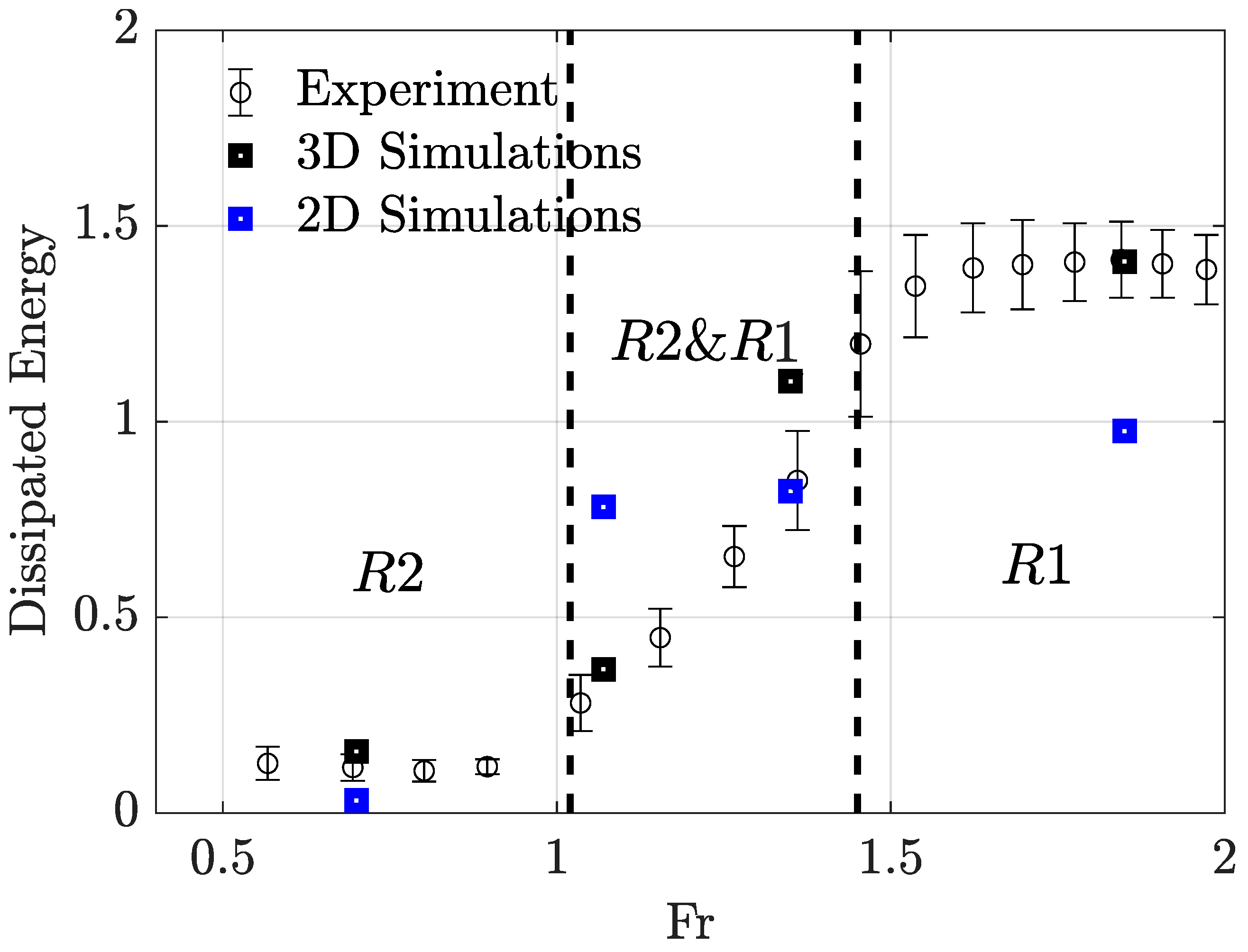
4. Results and Discussion

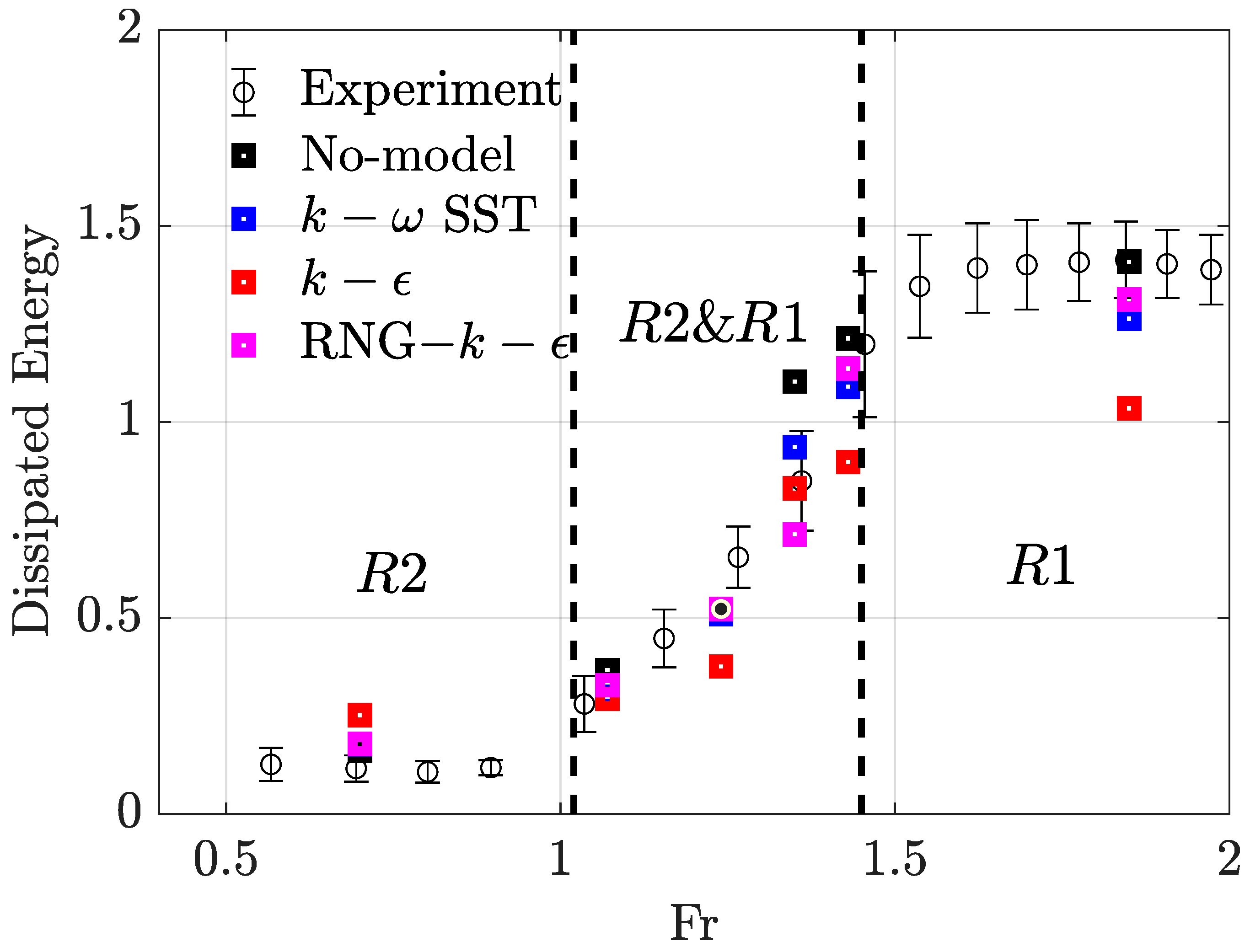
Figure 3 shows the experimental measurements of energy dissipation against $Fr$ number [59]. When comparing these results, it is important to consider that the dissipation is normalised by the amplitude squared. Thus, absolute dissipated energy always increases with the excitation amplitude, whereas the normalised values do not necessarily follow the same behaviour. The figure shows a clear trend and pattern of the damping as function of the excitation parameter, $Fr$. The figure shows three regions $R_2$ at low $Fr$, $R_1$ at high $Fr$ and an intermediate region $R_2\&R_1$. To understand why these three regions appear, it is important to consider the sloshing behaviour of the liquid at these regions. 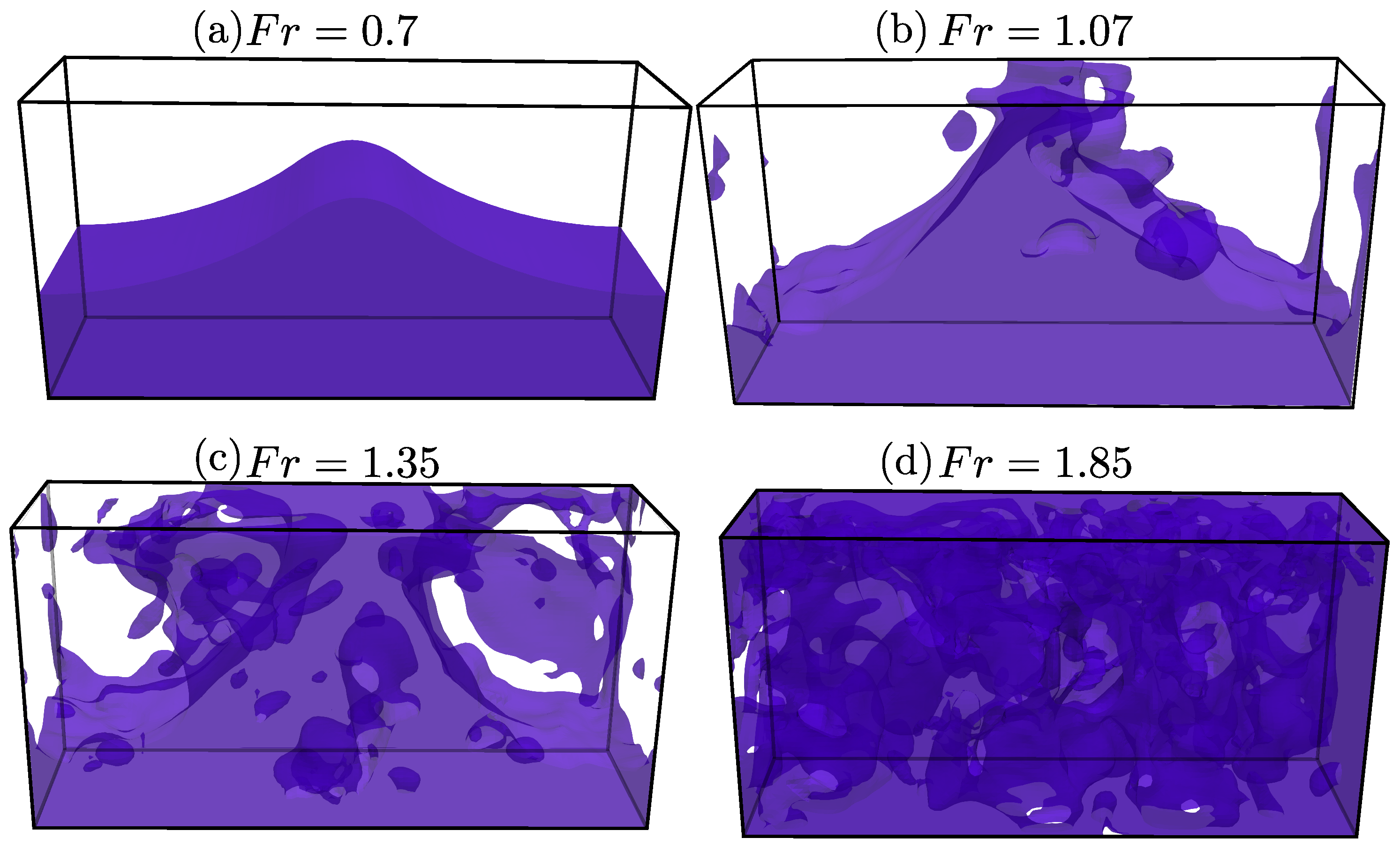Figure 4 shows a snapshot of the sloshing for a case at region $R_1$ ($Fr=0.7$) and another one in region $R_2$ ($Fr=1.85$). Two other cases at the start and the end of the intermediate region $R_2\&R_1$ ($Fr=1.07$ and 1.35, respectively) are also shown. These snapshots are produced by three-dimensional and no-model simulations. In the region $R_2$, the normalised dissipated energy is reasonably constant and small. The dissipation in the region induced by a single sloshing mode, can be seen in Figure 4a, with a small variation in the energy dissipation between cycles. As the excitation amplitude increases and enters the region $R_2\&R_1$, the liquid starts to impact the ceiling of the tank, and the liquid surface breaks. In this region, dissipation seems to grow linearly. Looking at Figure 4b,c it can be observed that the symmetric sloshing mode is still dominant. However, the dominance of a single sloshing mode in this region fades as the $Fr$ number increases, since the impact with the upper wall becomes stronger leading to and inducing turbulence. With further increase in the excitation amplitude, the response region $R_1$ is reached where the sloshing becomes very turbulent and the single sloshing mode vanishes. In $R_2$ region, the increase in normalised energy dissipation with the excitation level is slow, and reaches a saturation limit before falling down again.

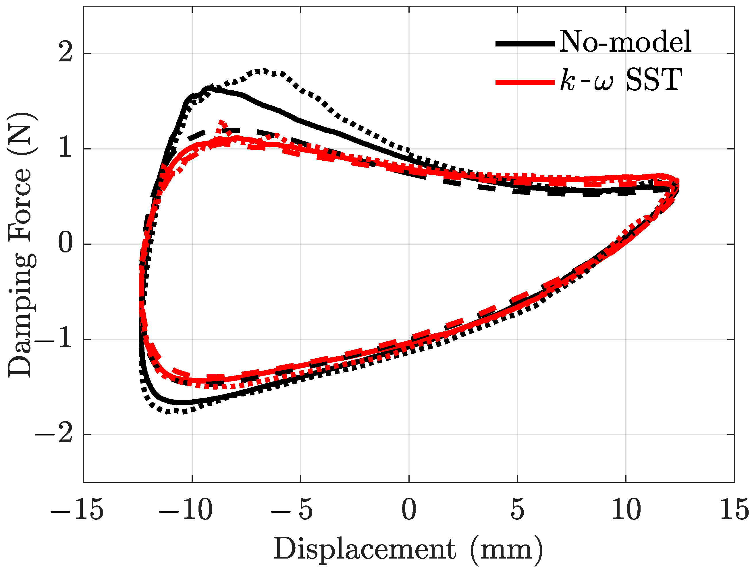
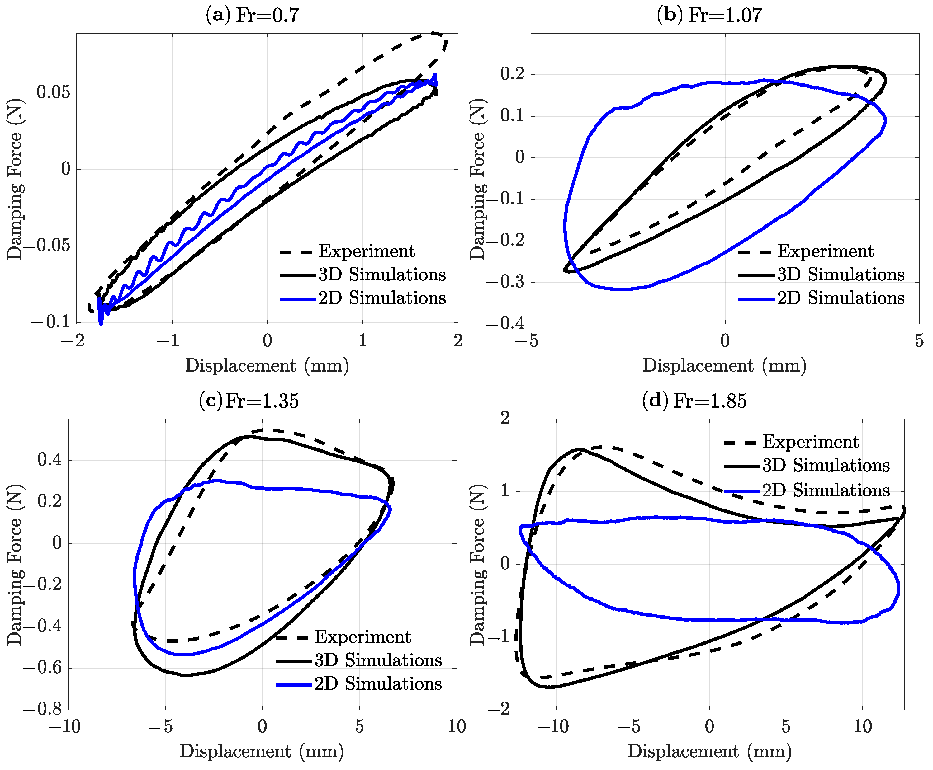
The dissipated energy is computed from the hysteresis of the mean damping force cycle. For a detailed comparison between the simulations’ setup, the hysteresis of the mean damping force cycle with displacement is shown in Figure 5 for four excitations, $Fr=0.7,1.07,1.35$ and $1.85$. Note that some simulations were conducted at $Fr$ numbers that do not exactly match their experimental counterparts, as the full experimental data were not available during the run time. However, the $Fr$ numbers are sufficiently close to produce a valid comparison between the cases, and the simulation cases are compared with the experimental case of the closest $Fr$ number, i.e., the simulated cases of $Fr=1.07$ are compared with the experimental case of $Fr=1.035$.

The experimental measurements of [59] show that at a low $Fr$ number of 0.7, the damping force hysteresis is symmetric. The damping force also has two peaks, one at the positive displacement and the other negative. In this case, the two peak forces are exerted at the upper and lower ends of the stroke, which also correspond to the maximum acceleration and deceleration of the fluid mass. As the excitation increases, the symmetry of damping force disappears and the location of the positive peak force shifts towards the negative displacement. At around $Fr=1.35$, the positive peak force occurs at zero displacement, or during a period of zero acceleration. A further increase in the $Fr$ number leads to the two peak forces happening during negative displacement. This behaviour mainly occurs from moving the tank with an acceleration higher than that of gravity, causing the liquid to impact the upper and lower walls [59].

4.1. Assessment of Two-Dimensional Simulations

Regarding the numerical simulations, the first test was to check whether two-dimensional simulations are sufficient to capture the dynamics of the sloshing. Without a turbulence model, two types of simulations were conducted. The first was a set of three-dimensional simulations at four excitation amplitudes corresponding to $Fr=0.7,1.07,1.35$ and $1.85$. The second was a set of two-dimensional simulations with the same $Fr$ numbers, where the breadth of the tank, $L_y$, is omitted. Figure 3 also compares these based on the estimated dissipated energy. The three-dimensional simulations can accurately estimate the levels and the trend of dissipation within the experimental error bounds. The two-dimensional simulations failed to produce reasonable results, except for in the case of $Fr=1.35$. Considering the overall behaviour of the two-dimensional simulations, it is likely that the result achieved at $Fr=1.35$ is actually a coincidence. This is further confirmed by examining the hysteresis of the damping force with the displacement. Figure 5 also compares the damping forces hysteresis computed by the two-dimensional and three-dimensional simulations. It is clear that the two-dimensional simulations do not reproduce the correct damping forces for all the cases, including the case with $Fr=1.35$ which bears a good estimation of the damping energy. The shape, peak values, and locations of the damping force are incorrectly estimated by the two-dimensional simulations. This further shows that relying on a single case or a single measured variable for validation of the efficacy of turbulent modelling can be misleading.

On the contrary, good agreement between computed damping forces and the reference data is achieved by the three-dimensional simulations. A detailed discussion of the three-dimensional no-model simulation results is shown later alongside a discussion of the simulations using turbulent modelling.

For high $Fr$ numbers, the deviation in results of the two-dimensional simulations is expected as the impact of the liquid onto the tank’s wall results in three-dimensional turbulent sloshing, and the sloshing is not dominated by a single sloshing mode in this case. At low excitation ($Fr<=1$), the fluid movement is dominated by the single and symmetric slowing mode, and hence the main fluid movements are symmetrical and two-dimensional. However, the two-dimensional simulation underestimated the dissipation. This can be attributed to the missing viscous force on the front and back walls (the walls parallel to the x–z plane), and in the case of low $Fr$, the viscous force accounts for around 20% of the total damping forces. As the excitation increases, the surface starts to break, creating three-dimensional patterns, and the symmetric sloshing mode becomes less dominant and the viscous force on the vertical wall also becomes less important. Therefore, where possible, it is crucial to validate the simulation setup under different conditions. For the excitation levels considered in the paper, three-dimensional simulations are adopted.

4.2. Assessment of Turbulence Models

To assess the performance of different turbulence models, energy dissipation estimations via three-dimensional simulations are amalgamated in Figure 6. All the presented models are able to produce good estimation of the energy dissipation for the low and medium excitation $Fr<1.5$ levels, except for the no-model simulation, which overestimates the dissipation for $Fr=1.35$. However, as the excitation increases, the no-model matches far better with the reference data, while the other turbulence models deviate. In all the high $Fr$ number cases, the standard K-$ϵ$ underestimated the dissipation, while the dissipation estimated with k-$\omega$ SST is slightly lower than the reference data, but still within reasonable uncertainty bounds. Considering the whole range of $Fr$ tested here, RNG K-$ϵ$ appears to have the best estimation of dissipated energy.

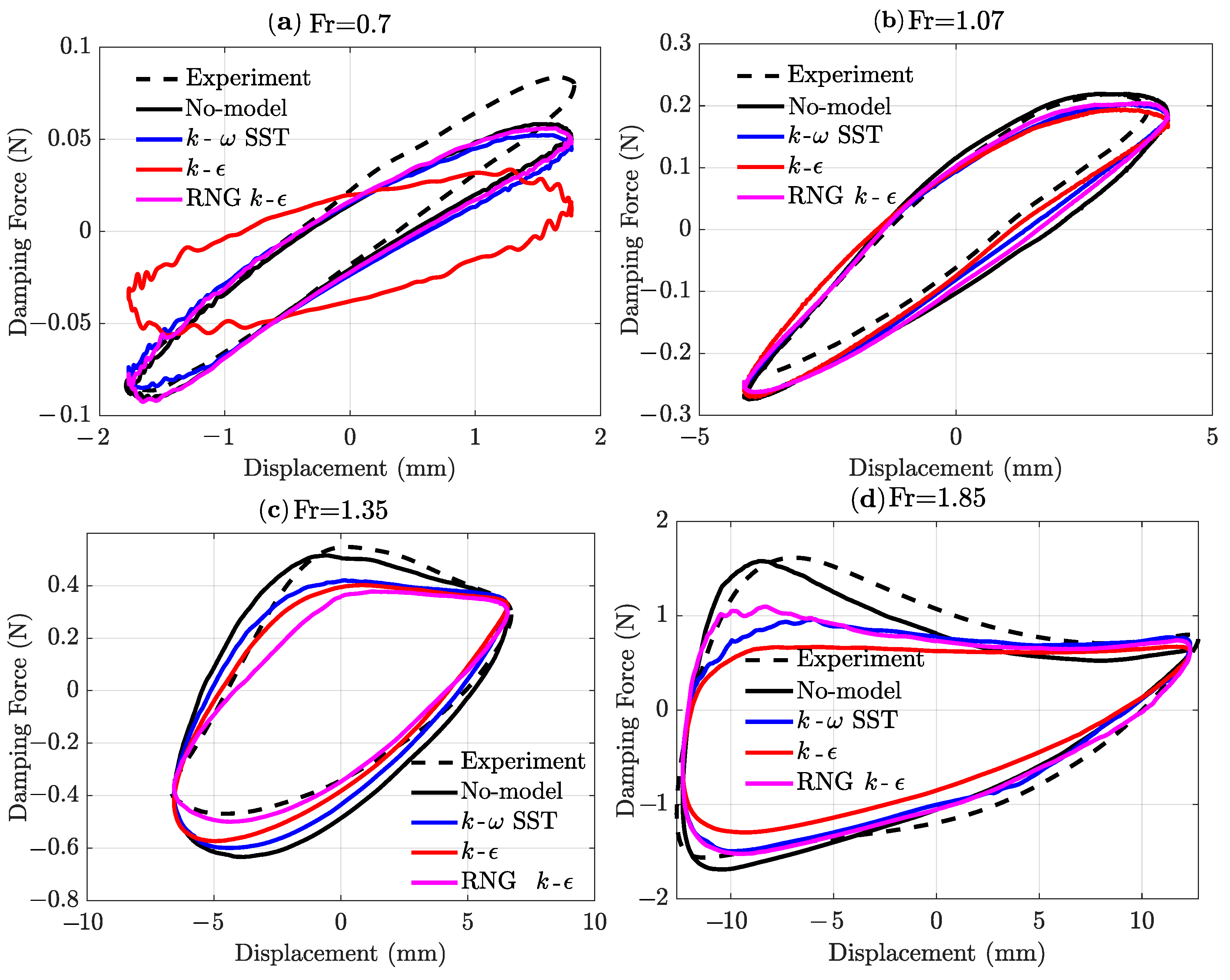
A good comparison between the models is to examine how well each depicts the damping force behaviour. The hysteresis of the damping forces as function of the displacement computed with the different models are shown in Figure 7. At $Fr=0.7$, the computed forces with the no-model, k-$\omega$ SST and RNG k-$ϵ$ models show inconsiderable differences, but the symmetric hysteresis is not obtained. The predicted forces accurately match the reference data during the negative stroke, but the damping forces are underestimated during the positive stroke. On the other hand, the standard k-$ϵ$ model preserved the symmetry of the damping force hysteresis, but significantly underestimated the peak force. For $Fr=1.07$, all models managed to demonstrate precise representation of the damping force for excitation. Note that the experimental case defines $Fr=1.035$ (not 1.07 as the simulations), which can explain the slight underestimation of the lower side of the hysteresis. The differences between the models become apparent at higher excitation, where the sloshing becomes violent and the effect of turbulence more prominent.

At $Fr=1.35$, all models fail to depict an accurate damping force throughout the whole cycle, in spite of the accurate estimation of the dissipation energy of some models. The no-model simulation produces a relatively accurate estimation of the damping force during the downward stroke, but significantly overestimates the magnitude of the damping force in the upward stroke, leading to an increase in the overall dissipated energy. On the other hand, the RNG k-$ϵ$ model underestimates the force in the downward stroke, but accurately computes the force in the upward stroke. The damping forces computed by the standard k-$ϵ$ model are lower than the reference values throughout the cycle, albeit the confined area of hysteresis agrees with the reference data, resulting in a good estimation of the dissipation energy.

Looking at the force hysteresis of the case with $Fr=1.85$, it is clear that the no-model simulation is the most accurate. The behaviour of the damping force, its peak values and locations agree very well with the experimental data. The damping force obtained by the turbulence models k-$\omega$ SST and RNG k-$ϵ$ follows the experimental data in the upward stroke, but in the downward stroke the peak force is underestimated. The magnitude of the damping force computed with the standard k-$ϵ$ is lower than the reference during the whole cycle.

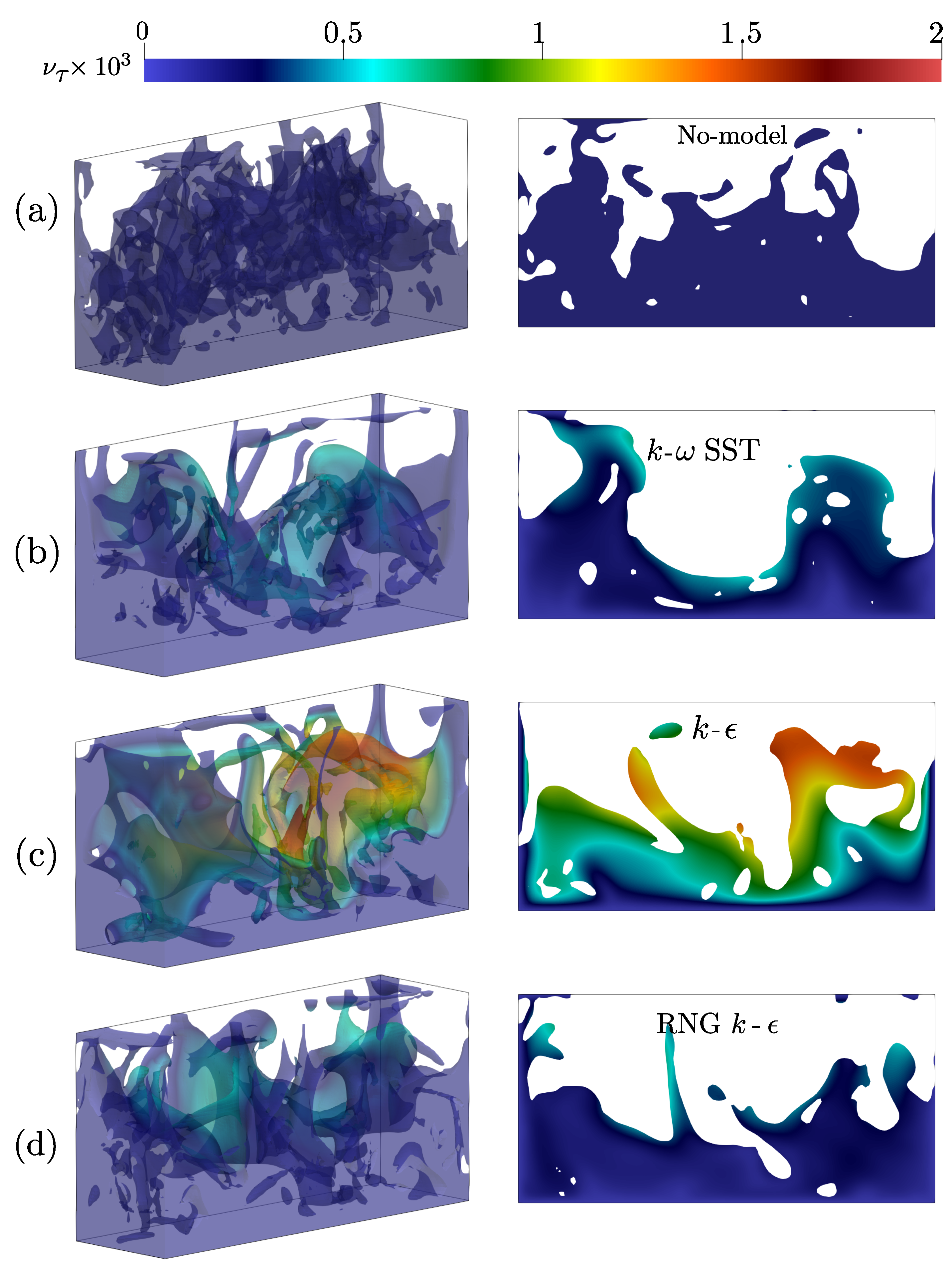
It appears that in the case of strong sloshing, the turbulent viscosity introduced by the turbulence models has a non-physical damping effect on the dynamics of the sloshing. This leads to a reduction in the liquid movement and reduction in the calculated damping effect of the sloshing itself. Figure 8 shows four snapshots of the liquid sloshing with $Fr=1.85$. The left-side figures are three-dimensional solid contours of $\alpha >=0.5$ and coloured with the turbulent viscosity. The right figures are middle-plane slices of the left figures. There are two main observations to be made. Firstly, turbulent viscosity applied by the standard k-$ϵ$ is the highest, and also affects most of the fluid domain, and the calculated values are significantly lower for k-$\omega$ SST and RNG k-$ϵ$. Secondly, looking at the shape of the sloshing liquid, the distribution of the liquid is the least complex for the standard k-$ϵ$ model, followed by k-$\omega$ SST and then RNG k-$ϵ$. The no-model simulation, on the other hand, produces the most complex sloshing behaviour. This suggests the existence of a reverse correlation between the turbulent viscosity and the strength of the predicted sloshing, i.e., the higher the turbulent viscosity, the less complex the sloshing dynamics becomes and hence the low estimation of the dissipated energy. This is consistent with the results above, where the lowest dissipation is obtained by the standard k-$ϵ$ model and the highest and most accurate dissipation is obtained by no-model simulations. It is worth noting that multiple snapshots were checked throughout the life-cycle of each simulation, and the same conclusion can be drawn.

The figure also shows that turbulent viscosity is highest at the interface due to the apparent overproduction of turbulent effects, which has a detrimental damping effect on the sloshing dynamics and leads to underestimation of the damping energy overall. The tested models suffer from this problem to different degrees, with the standard k-$ϵ$ model being the worst and RNG k-$ϵ$ the least affected. The phenomenon seems to impact the majority of two-equation closing models [50,58]. Although this problem has been known for over two decades [49], the standard RANS models have been used successfully in many studies [51,52,53,54,55,56,57], and the underlying cause of this problem is not fully understood [50]. Mayer and Madsen [49] proved that k-$\omega$ and k-$ϵ$ models are unstable in the region of potential flow beneath the surface, where the models can suffer from exponential growth in turbulent kinetic energy. Following Mayer and Madsen [49], Larsen and Fuhrman [50] performed stability analysis of a number of RANS turbulence closure models and showed that the models are unconditionally unstable. Understanding the underlying problem and more specifically, the differences between the models, is not trivial and requires detailed analyses of the design of each model. Although this is out of the scope of the present study, it will form the basis of what comes next.

To overcome this issue, Kamath et al. [30], Larsen and Fuhrman [50], Devolder et al. [68] proposed damping methods for turbulent viscosity at the interface, which improved the accuracy of the simulations. The aim of the current work is to investigate the capacity of the standard and the widely used RANS models to provide an accurate representation of violent sloshing. Modified version of the models with turbulent viscosity damping at the interface will be addressed in future work with the aim of capturing similarly complex fluid dynamics as the no-model method is able to reproduce whilst avoiding the obvious downside of this problem, requiring turbulence modelling in order to correctly capture its physics.

5. Conclusions

Simulations of sloshing-induced damping of partially filled water tanks under a harmonic oscillation motion are performed in this study. The simulations are conducted via the Volume of Fluid approach using the interFoam solver from the OpenFOAM v8 suite and using different turbulence models. The aim of the study is to investigate the efficacy of the most widely used turbulence models in providing an accurate representation of the flow under a range of sloshing conditions. The standard k-$ϵ$, RNG k-$ϵ$, k-$\omega$ SST and no-model are used in the simulation and compared against the experimental data of [59]. A range of excitation amplitudes are considered, starting from a Froude number of 0.7 and reaching 1.85. This corresponds to different sloshing patterns, ranging from single and symmetric mode of sloshing to a violent and turbulent sloshing. Therefore, this work can form the basis of future decision making on what modelling approaches are best suited for the sloshing problems at hand, with the understanding that no one approach is likely to work for all sloshing regimes.

It is found that the two-dimensional simulation fails to capture the complex dynamics in all cases, and hence the subsequent study is established using three-dimensional simulations. Comparison between the models is based on the estimated dissipated energy induced by the sloshing and a hysteresis of the damping force. In the case of weak and moderate sloshing, all of the turbulence models, except the standard k-$ϵ$, can accurately predict the damping force hysteresis and the energy dissipation. When the sloshing becomes more violent, the quality of the results obtained using any turbulence model degrades, especially in the prediction of the peak damping force. For the tested range of the excitation, the no-model simulations are found to have the best representation of the sloshing dynamics.

Analysing the added turbulent viscosity, it was found that the standard k-$ϵ$ is the most dissipative, followed by k-$\omega$ SST and then RNG k-$ϵ$. This suggests that the use of turbulence models, without an interface treatment, results in numerical damping that limits the strength of the sloshing that can be simulated and hence the modelled damping effect is reduced and not accurately captured compared to the no-model simulations. Another issue with the standard models is the non-physical and excessive dissipation near the interface, which can lower the efficacy of the model [30,50,68]. In future work, the effect of the treatment of turbulent viscosity at the interface will be addressed in order to improve the capability of the employed VoF approach to address complex sloshing flows as presented. Additionally, understanding the underlying cause of the differences between models and why some models are more dissipative at the interface than others presents an interesting topic for future work.