Article

Economic Optimal Scheduling of Wind–Photovoltaic-Storage with Electric Vehicle Microgrid Based on Quantum Mayfly Algorithm

College of Mechanical and Electrical Engineering, Shihezi University, Shihezi 832003, China
*
Author to whom correspondence should be addressed.
Appl. Sci. 2022, 12(17), 8778; https://doi.org/10.3390/app12178778
Submission received: 7 August 2022 / Revised: 25 August 2022 / Accepted: 28 August 2022 / Published: 31 August 2022
(This article belongs to the Special Issue Microgrids/Nanogrids Implementation, Planning, and Operation)

Abstract

:
The effectiveness of energy management systems is a great concern for wind–photovoltaic-storage electric vehicle systems, which coordinate operation optimization and flexible scheduling with the power grid. In order to save system operation cost and reduce the energy waste caused by wind and light abandonment, a time-sharing scheduling strategy based on the state of charge (SOC) and flexible equipment is proposed, and a quantum mayfly algorithm (QMA) is innovatively designed to implement the strategy. Firstly, a scheduling strategy is produced according to the SOC of the battery and electric vehicle (EV), as well as the output power of wind–photovoltaic generation. In addition, the minimum objective function of the comprehensive operation cost is established by considering the cost of each unit’s operation and electricity market sale price. Secondly, QMA is creatively developed, including its optimization rule, whose performance evaluation is further carried out by comparisons with other typical bionics algorithms. The advantages of QMA in solving the low-power multivariable functions established in this paper are verified in the optimization results. Finally, using the empirical value of the power generation and loads collected in enterprise as the initial data, the mayfly algorithm (MA) and QMA are executed in MATLAB to solve the objective function. The scheduling results show that the time-sharing scheduling strategy can reduce the system’s cost by 60%, and the method decreases energy waste compared with ordinary scheduling methods, especially when using QMA to solve the function.

1. Introduction

With the rapid development of the national economy, demand for fossil fuels is increasing. However, the output of traditional energy is limited, and the utilization of renewable energy has become the general trend. As new energy sources, wind and light are widely distributed and can be permanently used. They are characterized by low cost and strong environmental protection. Nevertheless, there are considerable random fluctuations of output power due to natural conditions, which affect the security and stability of the power system after grid connection [1,2,3]. Therefore, designing a stable and low-cost scheduling strategy based on the structure of the wind–photovoltaic-storage electric vehicle complementary power generation system has become a key issue. By coordinating wind–photovoltaic and flexible devices, we can ensure the reliability of the system, improve the economy, and increase environmental friendliness [4,5].
In the process of modeling, parameter uncertainty becomes a significant problem that threatens system security with the increasing scale of the microgrid. In order to solve this problem, robustness becomes one of the parameters worthy of study [6,7]. The improvement of robustness can make the system maintain its balance when it is disturbed, thereby reducing the loss caused by disturbances [8]. Meanwhile, some other power consumption units are introduced, such as electric vehicles (EVs) and fuel cells, on the basis of wind–photovoltaic-storage microgrid architecture, which can ensure the system maintains a stable operation by interacting power with other components when it is impacted [9,10]. In terms of the objective function, some microgrid systems, including fossil fuels, need to be considered regarding carbon emissions to reduce the environmental pollution caused by them [11]. Therefore, multi-objective functions combined with economic objectives and carbon emissions are established in recent studies. Furthermore, in order to ensure the normal operation of the microgrid system, it is necessary to ensure power conservation is met, and power flow constraints, including power flow calculation, should be added to the scheduling study [12,13]. Additionally, equipment parameters are important constraints to enable the system to operate under the superior performance of the equipment, thereby ensuring equipment safety and power quality.
In order to realize the scheduling strategy and accurately find the optimal value of the objective function, a variety of high-performance intelligent algorithm schemes based on biological habits are proposed, and verified in specific cases [14,15,16]. Bionics algorithms, such as the flying sparrow search algorithm, flower pollination algorithm, and other heuristic algorithms, are proposed and applied to practical problems [17,18,19]. Among them, as a new bionics algorithm, the mayfly algorithm (MA) has better optimization performance than the traditional intelligent algorithms. The integration of the advantages of various algorithms has significantly improved the optimization process in terms of speed and accuracy [20]. However, when it comes to high-dimensional complex problems, it is still difficult to jump out of local optimal regions simply by relying on its own mechanism, and the convergence accuracy of the algorithm is not high enough because the step size of the mayfly is too short when it moves. Based on the above shortcomings, logistic mapping is used to improve the optimization ability of mayfly individuals [21,22], or the learning factor is changed to improve the degree of self-adaptation [23].
In order to describe the research status of microgrid scheduling and its characteristics more clearly, the studies conducted for our paper, and other related studies, are summarized in Table 1, which is represented as follows:
Through the above table, it can be seen that the robustness and stability of the system are studied by some scholars. In these studies, robust model predictive control (RMPC) and other methods are used to deal with the uncertainties of renewable energy. In the microgrid system containing fossil energy, reducing carbon emissions is also an important issue that needs to be solved to improve the environmental protections of the system. More studies focus on the microgrid system containing EVs, namely the EVs charging and discharging states, as well as the stability of the EVs themselves.However, it is also worth studying how to interact with the microgrid while ensuring its stable operation. Meanwhile, some studies are aimed at improved algorithms, which have been greatly modified in optimization rate, convergence, and escape from local deadlock; however, there is still room for further improvement. Therefore, the problems that are concentrated on in this paper are represented as follow:
(1) The EV is taken as one of the dispatching objects, and its interaction state with the microgrid is judged according to its SOC. The microgrid system is able to make full use of power in this measure.
(2) The QMA algorithm raised in this paper is compared with the moth–flame optimization (MFO), grey wolf optimize (GWO), particle swarm optimization (PSO), whale optimization algorithm (WOA), sine cosine algorithm (SCA), and MA to verify its advantages, and is applied to the solution of the objective function.
The rest of the paper is organized as follows: The structure model of the microgrid is established in Section 2. Meanwhile, the scheduling strategy of each unit, as well as the objective functions with constraint conditions of economic dispatching regarding the microgrid, are established. In Section 3, the operation rules of the QMA are analyzed, and the comparison between various intelligent algorithms is realized. The algorithms are combined with the objective function in Section 4, and the economic scheduling of the microgrid in a specific area is carried out according to the actual situation. Section 5 summarizes the content and contributions of this paper, and puts forward prospects for future studies.

2. Microgrid Structure and Dispatching Strategy

2.1. Microgrid Structure

The model of the wind–photovoltaic-storage electric vehicle microgrid system is shown in Figure 1. Power output can be achieved by wind turbines and photovoltaic generations, while the load can only consume power. As flexible equipment, the consumption and production of electric energy can be realized by EVs and batteries. Meanwhile, energy interaction can be implemented by the accession of the microgrid to the main grid.

2.2. Scheduling Strategy Research

In this paper, in order to minimize the overall cost by dispatching each generation unit, the following requirements should be met in the scheduling strategy to ensure power supply reliability:
(1)
Maximize the utilization of wind and photovoltaic power generation, and maximize their output through reasonable scheduling;
(2)
Minimize the redundant power generated by wind and photovoltaic units to avoid energy waste;
(3)
The difference between wind–photovoltaic generation and the power consumption of the load depends on the energy interaction with batteries, EVs, and the main grid, and whether this can meet power balance constraints.The comprehensive cost can be further reduced to achieve economic optimization by selling electricity to the main grid and EVs.
In order to achieve the above requirements, the dispatching strategy aiming at the system economy is designed as follow: The output of wind power and photovoltaic generations are coordinated, and participate in the dispatching according to the state of the battery and EV on charge. Finally the power balance is realized through the interaction process with the main grid.
a. Wind and photovoltaic generation
The empirical output value of wind and photovoltaic generation is taken as the actual output power, and the scheduling is carried out after increasing the cost of wind and solar abandoning in order to reduce energy waste. The output power of wind and photovoltaic generation after dispatching is compared with the empirical value. If the output power is lower than the empirical value, the output power after dispatching can be used; otherwise, the empirical value has to be maintained.
b. Battery generation
Since photovoltaic and wind generation is affected by daily environmental changes, the charging and discharging process of batteries can meet the demand. According to power load trends within 24 h, power supply states are divided into peak, normal, and valley periods. Charging and discharging strategies are adopted based on the current period and the battery state of charge (SOC). The specific process is shown in Figure 2.
According to Figure 2, charging and discharging can be carried out only if the battery SOC is within a certain range. When the charging and discharging standard is reached by the battery, the interactive state is judged according to its SOC value and the time period. Thereby, the charging and discharging power is calculated. The specific calculation method is provided as follow:
P b e s s ( t ) = S O C x ( t ) C x
where the charging and discharging power of battery at time T is described as P b e s s ( t ) . The SOC of the battery at time T is shown as S O C x ( t ) , which is the scheduling target of the battery. The rated capacity of the battery collected from empirical data is defined as C x .
c. Electric vehicle
The output of an EV can be judged according to its SOC. If the SOC can maintain the normal operation of the vehicle, the power is outputted to the system; otherwise, the system’s power is consumed. The flow is expressed in Figure 3.
Similar to battery scheduling, the output state of EVs can be judged according to their SOC. The output of the SOC after scheduling, according to the idea shown in Figure 3, can be used for further calculations, and the specific expression is represented as follows:
P e v ( t ) = S O C e ( t ) C e
where interactive power between EVs and the microgrid at time T is given as P e v ( t ) . The SOC of the EV at time T is shown as S O C e ( t ) , and the fixed capacity of EV is expressed as C e .

2.3. Expression Construction

2.3.1. Objective Function

In this paper, objective functions are established for the economy of the wind–photovoltaic-storage electric vehicle microgrid system under a grid-connected operation. Consider the operation, maintenance, and investment cost of each unit in a system, and the cost of grid sales and purchases. Meanwhile, taking into account the operating costs of EVs and the cost policies issued by the government for new energy, the optimization goal can be achieved through relevant scheduling. The expression is as follows:
M i n i m i z e F ( x ) = F w v + F x F G F E V + F B T
where the operation and maintenance costs of wind and photovoltaic generation are represented as F w v . The power generation and investment costs of the battery are determined as F x . The power grid sales and purchase costs are simplified as F G . The operating costs of EVs and policy expenses related to new energy power generation are given as F E V and F B T . The decision variable of the objective function is the output power of each unit, which is the real number. Moreover, the specific coupling relationships between decision variables and objective functions (3) are shown in subsections a–e.
a. Wind and photovoltaic generation
The equipment loss, manual repair, and operating reserve storage costs are included in F w v , which can be expressed as follows:
F w v = t = 1 T C w P w f ( t ) + t = 1 T C v P v f ( t ) + F R E
where the operation and maintenance cost coefficients of wind and photovoltaic generation are defined as C w and C v , respectively. These coefficients are based on the ratio of the total operation and investment costs of the equipment to the total annual generated power within a year obtained in enterprise. The output power of wind and photovoltaic power generation is computed as P w f and P v f , respectively. The operating reserve storage cost is simplified as F R E , which can be expressed as follows:
F R E = C R E [ P v f ( t ) + P w f ( t ) ]
where the operating reserve storage cost coefficients of wind and photovoltaic generation are given as C R E .
b. Battery generation
In Equation (6), F x consists two parts, which are the acquisition and maintenance costs of batteries. The acquisition cost is converted into each work process, and the specific expression is calculated as follows:
F x = F c a p C P b e s s T n | t = 1 T P b e s s ( t ) | + K o P b e s s , m a x 365 + K M 1 Δ t P b e s s ( t ) Δ t
where the acquisition cost and depreciation coefficient are defined as F c a p and C, respectively. The annual operating cost coefficient and hours are represented as K o and T n , respectively. P b e s s and P b e s s , m a x are battery-rated power and maximum charge and discharge power, respectively. Meanwhile, the maintenance cost coefficient is described as K M , and the duration from the beginning to the end of charging and discharging the battery is shown as T.
c. Interaction with main grid
The microgrid system can interact with the main grid when the power is vacant or redundant. When the interactive power is positive, the power is purchased from the main grid; otherwise, the interaction cost F G is the sum of the two. The equation is simplified as follows:
F G = t = 1 24 P g r i d ( t ) C p r i c e , g r i d
where P g r i d ( t ) refers to interactive power with the main grid, and the time-sharing sale and purchase price of the main grid is expressed as C p r i c e , g r i d .
d. Policy of government
Subsidies are paid for wind and photovoltaic generation, which encourage companies to adopt new sources of electricity. Meanwhile, fees are charged for energy waste to reduce the energy loss caused by wind and solar discarding. The formula is computed as follows:
F B T = t = 1 T C q [ P w y ( t ) + P v y ( t ) P w y ( t ) P v y ( t ) ] S b t
where the wind and solar discarding coefficient is given as C q and S b t , which represents the government subsidy. The actual utilization power of wind and photovoltaic generation is determined as P w y ( t ) and P v y ( t ) , respectively.
e. Electric vehicles
As a client device, the cost of selling and purchasing power to the microgrid is mainly included in the cost of EVs. The specific expression is given as follows:
F E V = t = 1 24 P E V ( t ) C p r i c e , E V
where the electricity purchase price of an EV is defined as C p r i c e , E V .

2.3.2. Constraint Condition

In order to ensure the safe and stable operation of the grid system, the power balance should be regarded as the basic constraint condition, and the output power and SOC of flexible devices should be limited to ensure the normal operation of equipment.
a. Power balance
In any period of time, all output, load, flexible device charging and discharging, and interaction powers between the microgrid system and the main grid should be kept in balance, and the constraint equation is given as follows:
P w y ( t ) + P v y ( t ) + P g r i d ( t ) + P x ( t ) + P E V ( t ) = P l o a d ( t )
where P x is the charging and discharging power of the battery, and the total load is expressed as P l o a d .
b. Wind and photovoltaic generation
Due to the limitations of the equipment parameters, the output power of wind and photovoltaic generation is within a certain range. Meanwhile, in order to ensure the normal operation of the system when the power required surges, it is necessary to add operating reserves. In detail, 30% of power generated by wind and photovoltaic power generation is stored, and the rest is the maximum power supplied to the system. Furthermore, the change of power in each time period should also be constrained in a certain range. Therefore, the relevant constraints are set as follows:
0 P w y ( t ) 0.7 P w f ( t ) 0 P v y ( t ) 0.7 P v f ( t ) R w d o w n δ t δ P w R w u p δ t R v d o w n δ t δ P v R v u p δ t
where the adjustable power amplitude of wind and photovoltaic generation in a certain period is represented as δ P w and δ P v , respectively. The downward climbing rate of wind and photovoltaic generation during adjustment is expressed as R w d o w n and R v d o w n , respectively. Meanwhile, R w u p and R v u p give the upward climbing rate for wind and photovoltaic generation during adjustment, respectively. The adjustment time is represented by δ t .
c. Flexible generation
Batteries are not only constrained by power, their safety performance and service life are affected by their SOC, and the operation of an EV is also affected by its SOC. Specific conditions are simplified as follows:
S O C e m i n S O C e ( t ) S O C e m a x S O C x m i n S O C x ( t ) S O C x m a x 0 P b e s s , t ( t ) P b e s s , m a x
S O C e m i n , S O C x m i n , S O C e m a x , and S O C x m a x are the upper and lower limits of their SOC.
In addition, to ensure the safe and stable operation of batteries, the charging and discharging rates should be controlled within a certain range. The specific constraints are shown as follows:
δ S O C x 0.2
where the adjustable range of a battery’s SOC in each period is expressed as δ S O C x .

3. Improved Mayfly Algorithm

3.1. Traditional Mayfly Algorithm

The MA is a bionics algorithm derived from the social behavior of the mayfly. Inspired by the movement mode and reproduction process of female and male populations, the optimal and suboptimal individuals in each population are selected. Meanwhile, the optimal offspring generation is obtained through mating between the optimal male and female individuals, and the suboptimal offspring generation is obtained in the same way. The direction of movement of each mayfly is influenced by the dynamics of individual and collective optimal positions, and female mayflies target male mayflies towards their positions.
a. The movement of male mayfly
The flight mode of male mayflies is similar to the movement mode of birds in a particle swarm algorithm, and the direction and distance of male mayflies are adjusted according to their own flight experiences and that of individuals around them. The specific method is shown as follows:
x i n + 1 = x i n + v i n + 1
where x i n and v i n are the current position and speed, respectively, of the male mayfly i on the nth search. The values are calculated as follows:
v i j n + 1 = v i j n + α 1 e β l p 2 ( p b e s t i j X i j n ) + α 2 e β l g 2 ( g b e s t i j X i j n )
Because male mayflies perform a dance on the surface of water to attract females, the position of the male mayflies is constantly changing, meaning they do not build a high speed. v i j n is the speed of the nth search of the mayfly i at j dimension, and x i j n is the position at that time. α 1 and α 2 are estimated from the positive attraction coefficients of social interaction, and β is the visibility coefficient of the mayfly. Meanwhile, the optimal locations of the individual and collective mayflies are expressed as p b e s t i j and g b e s t i j , respectively. Additionally, the distances from current position to p b e s t i j and g b e s t i j are defined as l p and l g , respectively, and are calculated as follows:
x i X i = j = 1 n ( x i j X i j ) 2 2
For the best mayfly in the population, a fixed dance pattern is needed to be maintained. Meanwhile, a random element is introduced to ensure that the speed is constantly changing. The calculation is described in this case as follows:
v i j n + 1 = v i j n + d × r
where the dance coefficient is simplified as d, and r is the random natural number within [−1, 1].
b. The movement of female mayfly
The movement of the female mayfly depends on the attraction of the male mayfly, and their position renewal depends on the increase of speed, which can be expressed as follows:
y i n + 1 = y i n + v i n + 1
The speed update is a certain process, which means that in order to ensure the quality of offspring, the best female needs to be attracted by the best male, the second-best female by the second-best male, and so on. The speed update expression is given as follows:
v i j n + 1 = v i j n + α 2 e β l f 2 ( x i j n y i j n ) v i j n + g × r
where the position of the female mayfly is expressed as y i j n , the random walk coefficient of the female mayfly is represented as g, and l f is determined by the distance between the male and female mayflies.
c. The mating of male and female mayflies
In the process of parent mating, the optimal and suboptimal individuals in the male and female populations should be selected for mating and reproduction based on their fitness functions. The results of interbreeding, which produces the optimal and suboptimal offspring, are calculated as follows:
o f f s p r i n g 1 = L × m + ( 1 L ) × f m o f f s p r i n g 2 = L × f m + ( 1 L ) × m
where the male and female in the parent generation are represented as m and f m , respectively, and L is a random natural number within a specific range.

3.2. Ma with Quantum Idea

The traditional MA can find the optimal value in a single-peak function accurately by taking advantage of the characteristics in mayfly reproduction. However, with regard to the large population and complicated process, the search speed is slow and the convergence is not fine. Meanwhile, it is easy to fall into local deadlock when dealing with multi-peak functions. Therefore, the quantum idea is introduced on the basis of a traditional MA, thereby forming the QMA. Because the position and velocity of the mayfly cannot be determined simultaneously in quantum space, the wave function is used to represent the position of the mayfly, and the Monte Carlo method is used to solve the problem. The particle update expression is shown as follows:
m b e s t n = 1 N i = 1 a P b e s t i n ( i = 1 n ) P i t = γ × P b e s t i n + ( 1 γ ) × g b e s t n X i n + 1 = P i n ± ε | m b e s t n x i n | log 1 a
where the numbers of individuals and iterations are represented as N and n, respectively. m b e s t n is the average historical optimal position of the male mayfly, and P i n is obtained from the updated position of the ith male mayfly in the nth iteration. r and a are uniformly distributed values within (0,1), and c is the final random motion parameter.
The execution steps of the QMA are given as follows:
Step 1: Initialize the positions of the female and male mayflies in the space.
Step 2: Calculate the average optimal location m b e s t of the male mayflies according to the first equation of (21).
Step 3: Calculate the fitness value and sorting according to Formula (3), and compare with the previous iterative value. If the current function value is less than the previous iteration, the current mayfly position is updated for the individual optimal position, otherwise it keeps the previous iteration. Hence, the optimal male individual p b e s t and collective locations g b e s t are obtained.
Step 4: Calculate the new positions of the female and male mayflies according to Formula (18) and the second equation of (21), respectively, and mate in sequence.
Step 5: Calculate the fitness function and update p b e s t and g b e s t .
Step 6: Repeat Step 2 to 5 until the stop condition is met.
The QMA flow chart is shown in Figure 4.

3.3. Performance Analysis of Qma

In order to verify the superiority of the QMA, the single-peak and multi-peak functions are tested by MFO, GWO, PSO, WOA, SCA, MA, and QMA in this section. We combine the biological habits and existing literature on each algorithm, and the initialization parameters and test functions are shown in Table 2 and Table 3, respectively. Meanwhile, to ensure the effectiveness of the comparison results, the number of biological populations in all bionics algorithms is set as 10. The function expression is represented by Fun, and the expression dimension is expressed as Dim. L b and U b are the upper and lower boundaries of the variables, respectively.
Sphere function is represented as F1, which is a typical single-peak function. The optimization time and local search ability of the algorithm can be effectively verified in this type of function. The Rastrigrin function is simplified as F2, and the validity of breaking away from local deadlock in the algorithm can be proved in this multi-peak function. The performances of different optimization algorithms in solving these two functions are expressed in Table 4. The iteration curves of these functions run once are shown in Figure 5 and Figure 6.
As can be seen from the Figures and Table, the average value, variance, and standard deviation of the different algorithms after 30 iterations in solving functions are different. The optimal value can be found quickly in the WOA, MFO, and GWO algorithms once they get rid of local deadlock when solving multi-variable functions. However, it is easy for them to fall into a local optimum, which is greatly affected by the number of iterations and randomness. Hence, it is not suitable for these algorithms to solve such functions. Compared with the SCA, PSO, and MA algorithms, although the convergence speed is not fast as the above algorithms, the rate is stable, and it is not easy to get into local deadlock. They have good performance in solving multi-variable lower-power functions, and MA has the most stable optimization rate among them. On the basis of MA, the stability of optimization is improved further in the QMA, and the optimal solution of the objective function can be found better in it. In the function where the optimal value is zero, the optimal value found by the QMA in the optimization process is lower than other algorithms, and the performance is more stable with little variance. In the scheduling problem of the microgrid, many variables are obtained in an economic objective function, and the stability of optimization is needed to ensure this. Hence, it is suitable for the QMA to find the optimal value of the economic scheduling function based on the microgrid established in this paper.

4. Simulation Analysis of Microgrid

Entering into cooperation with an enterprise, a typical winter day in the region where the enterprise is located is taken as an example to make economic scheduling. The actual data, such as wind–photovoltaic power and residential electricity consumption obtained from enterprise, are input as empirical values. Based on the economic scheduling objective function of the wind–photovoltaic-storage electric vehicle microgrid established in 
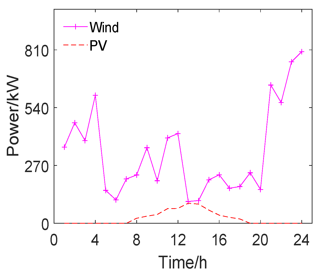
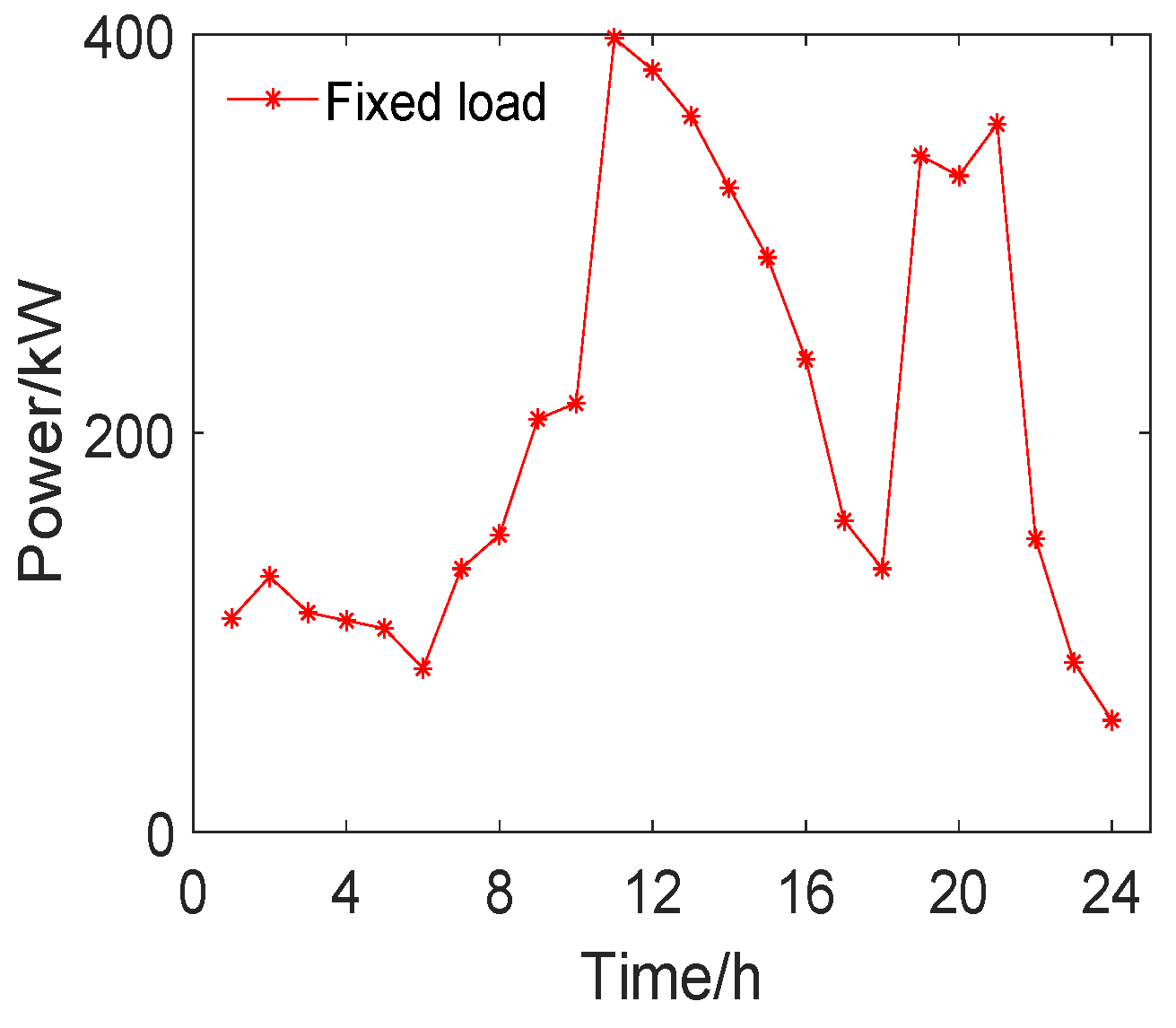
Section 2, the QMA and MA algorithms are used to solve it. The algorithms are invoked, combining with the microgrid economic objective function, and the number of the population in the algorithms is set as 100 after several simulations. In this condition, the objective function the algoriths can commendably solve the problems regarding optimization speed and convergence. Hence, the output power of each unit within 24 h is obtained. The output empirical values of wind and photovoltaic generation collected from enterprise are expressed in Figure 7, and the empirical values of residential electricity consumption are shown in Figure 8.
Under the load conditions, the optimization algorithms are used in this paper to find the minimum output cost under the condition of maintaining the security and stability of the system. Combined with empirical data obtained from the enterprise, the status of various components in the microgrid and the equivalence coefficient are shown in Table 5 and Table 6. The related parameters of the time-of-use price are shown in Table 7.
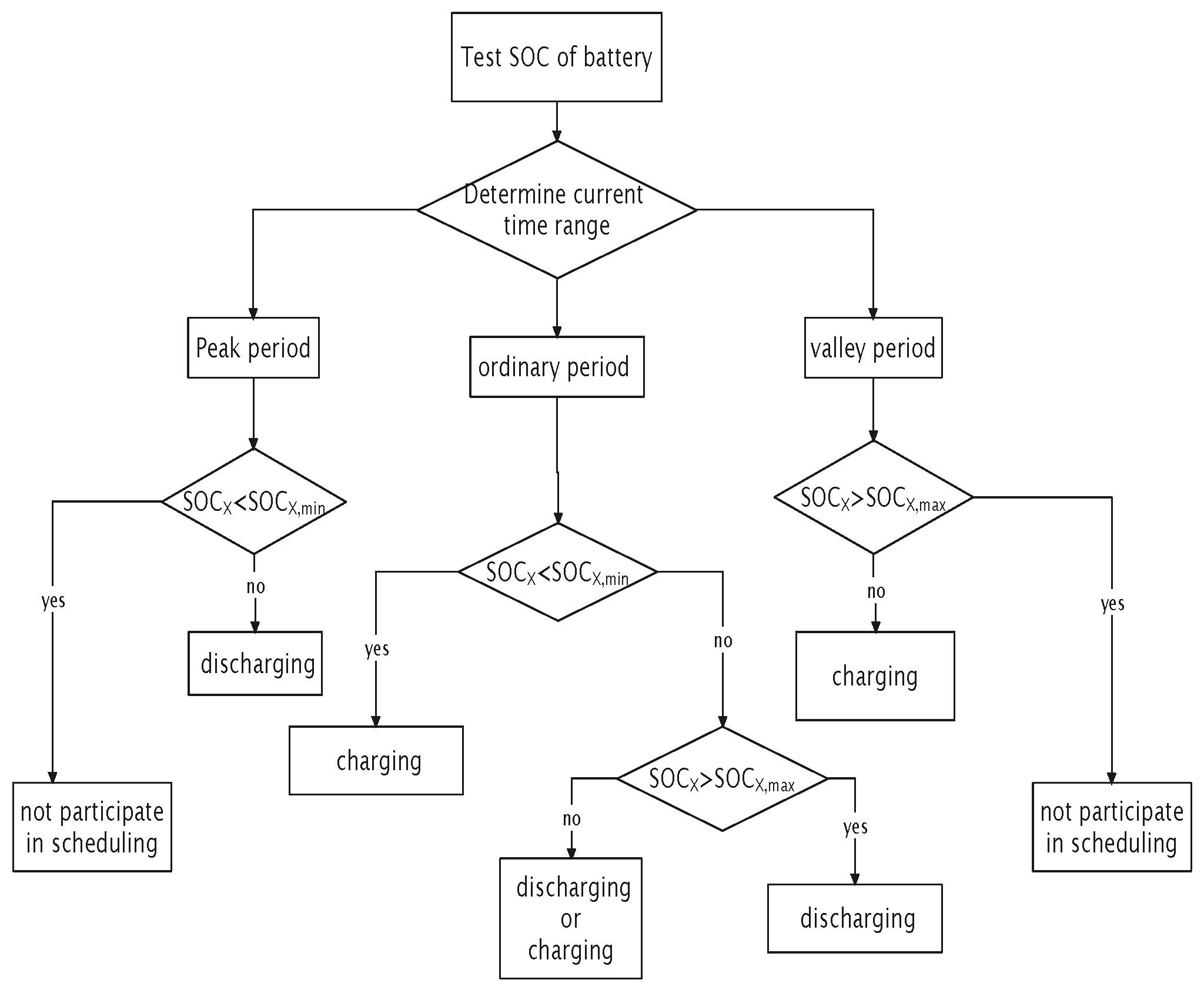
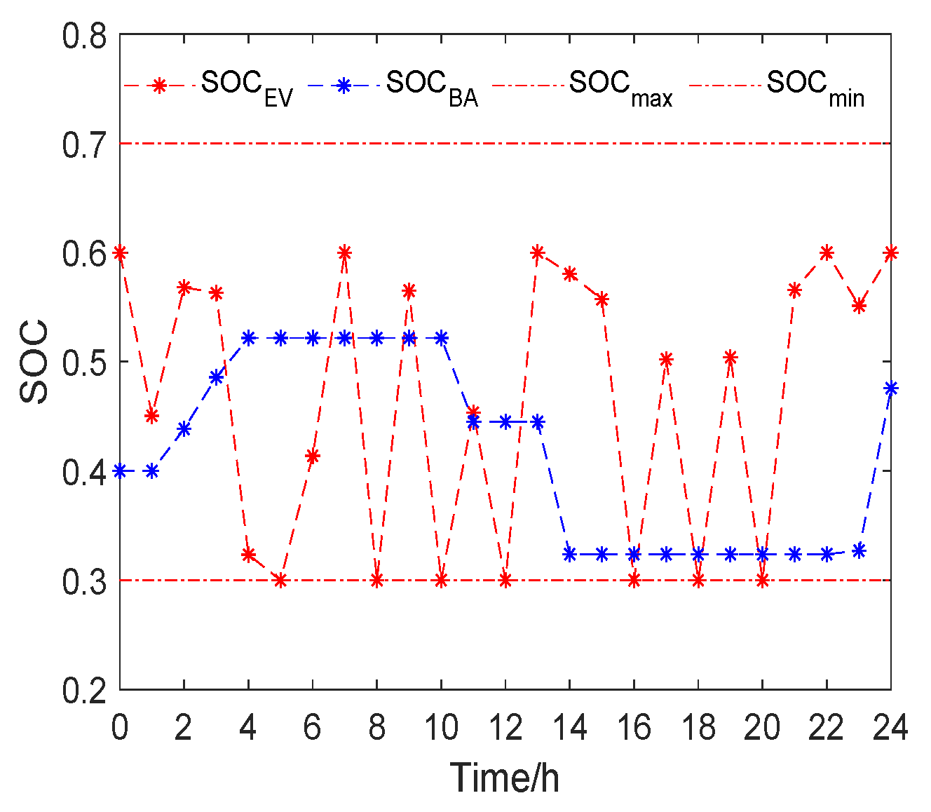
When MA and QMA are used to solve the objective function, the SOC of the battery and EV are shown in Figure 9 and Figure 10, respectively. The recharging of the battery is represented as an increase in SOC; otherwise, the battery delivers power to the grid. When the SOC of the battery is between 0.3 and 0.7, it can maintain its operation in the best condition. Taking 
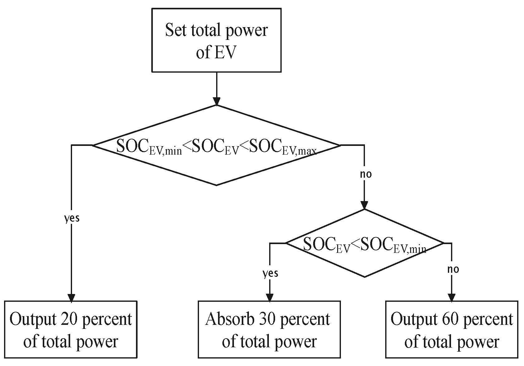
Figure 10 as an example, when QMA is used to solve the system objective function, the battery is charged in three time periods: 1:00–2:00, 15:00–16:00, and 23:00–24:00. Meanwhile, discharge is performed in four time periods: 10:00–12:00, 14:00–15:00, 18:00–19:00, and 20:00–21:00. The rest of time, the battery remains neither charged nor discharged. Furthermore, if there is more than one EV in the area, their SOC is not continuous with great fluctuations, and they can operate normally when the SOC is within the range of 0.3 to 0.7.
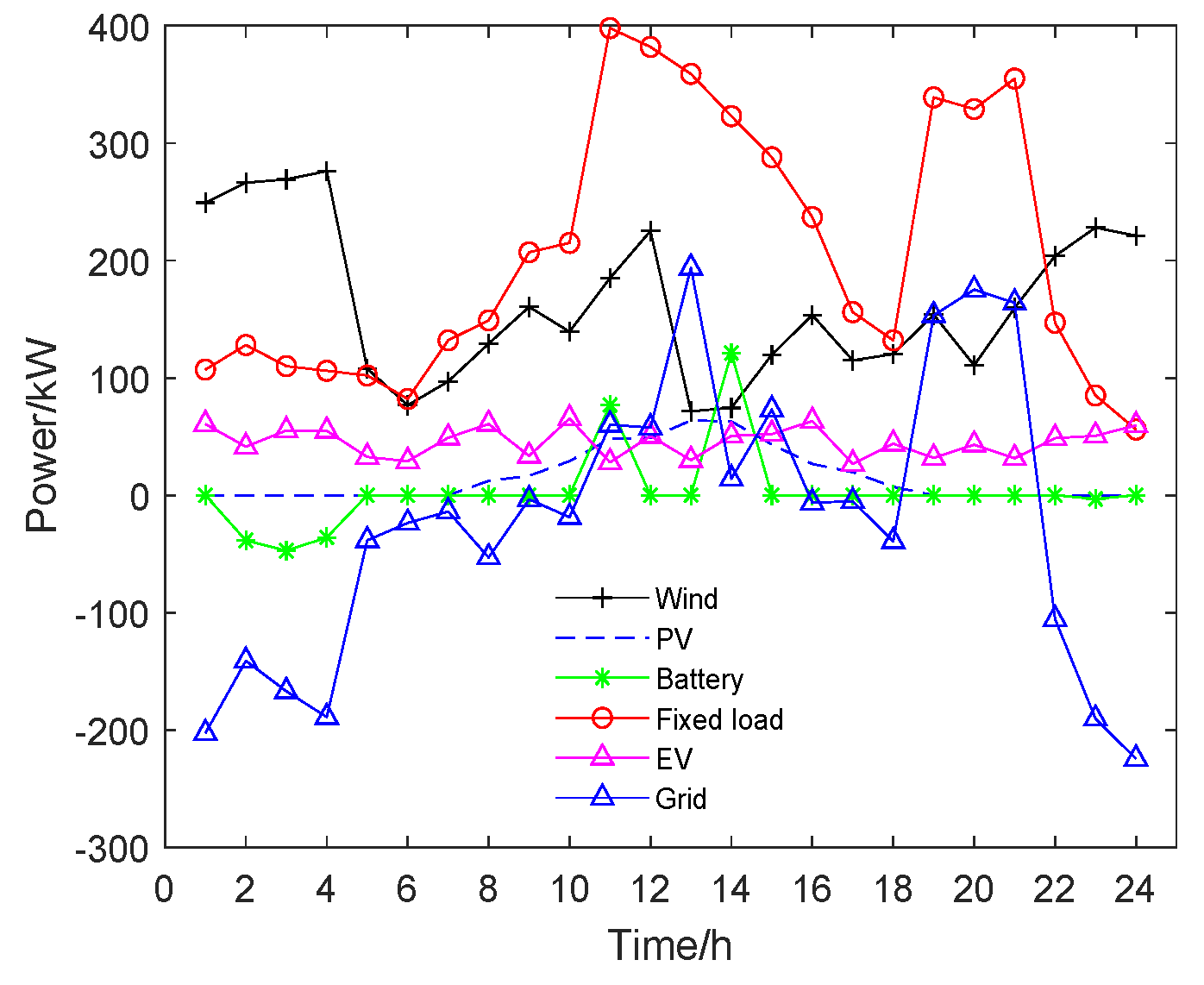
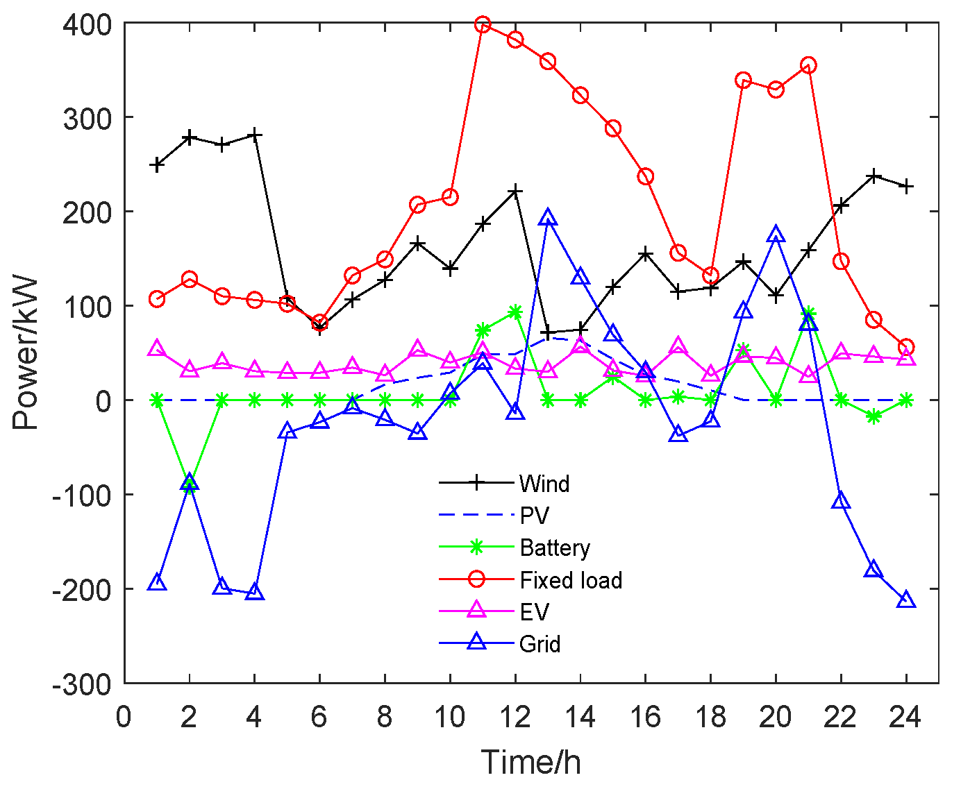
The output of each unit when MA and QMA solve the objective function is represented in Figure 11 and Figure 12, respectively. The load power curve is the absolute value of consumed power.
Abundant power is generated by wind turbines within 0:00 to 4:00, and the microgrid consumes redundant power by interacting with the main grid. From 4:00 to 11:00, the output power of wind–photovoltaic generation and EVs supplies power to load; meanwhile, the redundant power is consumed by the main grid. From 11:00 to 16:00 is the peak period of electricity consumption. During this time, almost all power generation is used to maintain the power required by load. The load demand gradually decreases from 16:00 to 18:00 and reaches the peak again from 18:00 to 21:00. In this period, wind generation and EVs are in a power output state, while photovoltaic generation occasionally outputs power, and the interaction with the main grid absorbs or transfers power to the main grid as the load requires. Finally, load demand drops from 21:00 to 24:00, and wind generation and EVs mainly send out power and feedback to the main grid.
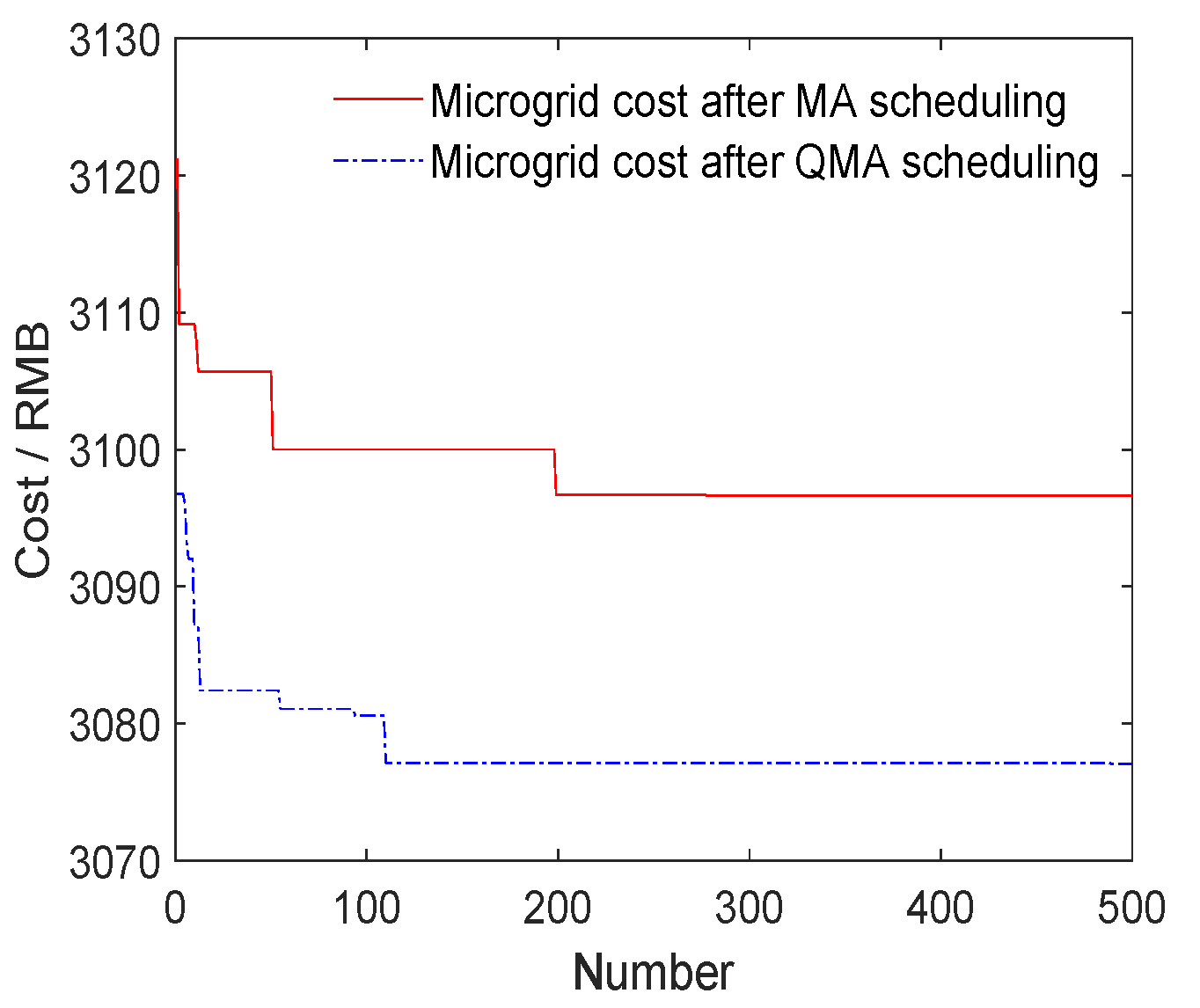
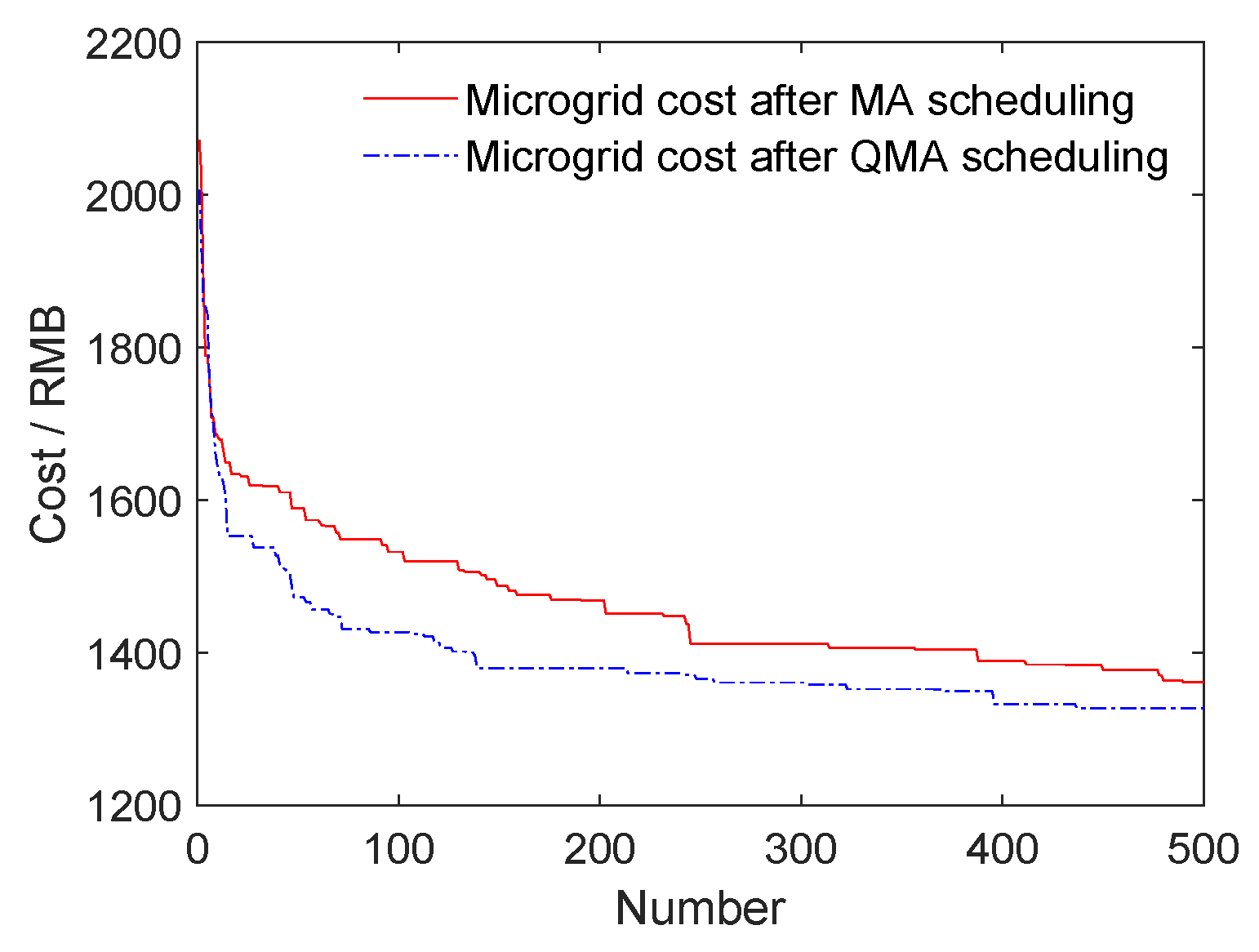
When the output power is at 10% of its maximum capacity it is stored by the battery, and the wind–photovoltaic generation produces power according to the empirical value. The operation cost of the microgrid is shown in Figure 13; furthermore, the operation cost of the microgrid obtained by solving the objective function using the scheduling strategy in Section 2 is shown in Figure 14.
The results of the value and standard deviation of MA and QMA after 100 and 500 iterations are shown in Table 8. In terms of these results, the operating costs under the empirical value are higher than the costs after participating in scheduling according to the strategy. Moreover, the optimization rate of QMA is higher than that of MA, and the optimal solution found by the improved algorithm after 500 iterations is obviously better than the solution obtained before the improvement.
In summary, the scheduling strategy provided in this paper can effectively improve the economy of the microgrid system, and the improved QMA has a high level of superiority when solving the objective function.

5. Conclusions

According to the operation state of a wind–photovoltaic-storage electric vehicle microgrid connected to the grid in a certain area, a time-sharing scheduling strategy is designed in this paper; furthermore we established the minimum cost objective function according to economic requirements and constraints, such as wind and light abandonment. Meanwhile, a QMA algorithm is innovatively proposed and applied to the solution of the objective function. In summary, the main conclusions of this paper are expressed as follows:
(1)
The SOC of the EV and battery is taken as a scheduling object, and it is scheduled in combination with the current period, thereby obtaining the interaction power between the flexible equipment and microgrid. Furthermore, the output power of wind and photovoltaic generation is limited within the empirical value and, accordingly, the energy waste caused by wind and light abandonment is reduced. This scheduling method not only reduces energy waste but also decreases the system cost by about 60%;
(2)
On the basis of the MA, the quantum idea is introduced, and the QMA is proposed. Comparing the performance of the QMA with six other intelligent algorithms in typical functions optimization, the superiority of the QMA is clearly seen. Meanwhile, the QMA is applied to the objective function established in this paper. The cost of the system can be reduced by about 2%, which is considerable for the microgrid system.
In future research, new energy devices need to be taken into account, and the robustness of the system should also be paid attention to because of the increasing complexity of the system. Meanwhile, in order to make managers more intuitive, namely to understand the operation state of the system, the connection between information management and the physical layer should be strengthened. It is necessary to study the use of hierarchical scheduling, source and charge interactions, and other methods to meet the needs of different managers.

Author Contributions

X.L. wrote the manuscript, designed the scheduling strategy, drew the flow chart and table, and performed the simulation experiment and analysis. M.Z. supervised the study, helped obtain data, and checked the contents of the manuscript. Z.W. verified the simulation data and contributed to the writing and typesetting of the manuscript. M.L. provided practical suggestions and evaluated the feasibility of the application. All authors have read and agreed to the published version of the manuscript.

Funding

This work was Supported by the Natural Science Foundation of China under Grant No. 61563045.

Institutional Review Board Statement

Not applicable.

Informed Consent Statement

Not applicable.

Data Availability Statement

Not applicable.

Acknowledgments

Thanks to the electric power enterprises in Liaoning Province for providing data support for this research.

Conflicts of Interest

The authors declare no conflict of interest.

Acronyms

The following acronyms are used in this paper:
MAMayfly algorithm
QMAQuantum mayfly algorithm
MFOMoth–flame optimization
GWOGrey wolf optimizer
WOAWhale optimization algorithm
SCASine cosine algorithm
PSOParticle swarm optimization
EVElectric vehicle
SOCState of charge

References

  1. Rui, T.; Li, G.; Wang, Q.; Hu, C.; Shen, W.; Xu, B. Hierarchical Optimization Method for Energy Scheduling of Multiple Microgrids. Appl. Sci. 2019, 9, 624. [Google Scholar] [CrossRef]
  2. Wang, J.; Li, K.-J.; Javid, Z.; Sun, Y. Distributed optimal coordinated operation for distribution system with the integration of residential microgrids. Appl. Sci. 2019, 9, 2136. [Google Scholar] [CrossRef]
  3. Harsh, P.; Das, D. Energy management in microgrid using incentive-based demand response and reconfigured network considering uncertainties in renewable energy sources. Sustain. Energy Technol. Assess. 2021, 46, 101225. [Google Scholar] [CrossRef]
  4. Zhang, Z.; Wu, J.; Luo, Z.; Xu, J.; Jin, X.; Li, H. Optimal Scheduling for Independent AC/DC Hybrid Microgrid Considering Operation Characteristics of Energy Storage. Power Syst. Autom. 2018, 42, 118–125. [Google Scholar]
  5. Hakimi, S.M.; Hasankhani, A.; Shafie-Khah, M.; Lotfi, M.; Catalão, J.P. Optimal sizing of renewable energy systems in a Microgrid considering electricity market interaction and reliability analysis. Electr. Power Syst. Res. 2022, 203, 107678. [Google Scholar] [CrossRef]
  6. Abdolrasol, M.G.M.; Hannan, M.A.; Hussain, S.M.S.; Ustun, T.S.; Sarker, M.R.; Ker, P.J. Energy Management Scheduling for Microgrids in the Virtual Power Plant System Using Artificial Neural Networks. Energies 2021, 14, 6507. [Google Scholar] [CrossRef]
  7. Carli, R.; Cavone, G.; Pippia, T.; De Schutter, B.; Dotoli, M. Robust Optimal Control for Demand Side Management of Multi-Carrier Microgrids. IEEE Trans. Autom. Sci. Eng. 2022, 19, 1338–1351. [Google Scholar] [CrossRef]
  8. Melhem, F.Y.; Grunder, O.; Hammoudan, Z.; Moubayed, N. Energy Management in Electrical Smart Grid Environment Using Robust Optimization Algorithm. IEEE Trans. Ind. Appl. 2018, 54, 2714–2726. [Google Scholar] [CrossRef]
  9. Shi, R.; Zhang, P.; Zhang, J.; Niu, L.; Han, X. Multidispatch for Microgrid including Renewable Energy and Electric Vehicles with Robust Optimization Algorithm. Energies 2020, 13, 2813. [Google Scholar] [CrossRef]
  10. Mbuwirabc, B.; Spiessensab, F.; Deconinckac, G. Distributed optimization for scheduling energy flows in community microgrids. Electr. Power Syst. Res. 2020, 187, 106479–106490. [Google Scholar] [CrossRef]
  11. De, M.; Das, G.; Mandal, K. An effective energy flow management in grid-connected solar–wind-microgrid system incorporating economic and environmental generation scheduling using a meta-dynamic approach-based multiobjective flower pollination algorithm. Energy Rep. 2021, 7, 2711–2726. [Google Scholar] [CrossRef]
  12. Scarabaggio, P.; Carli, R.; Dotoli, M. Noncooperative Equilibrium Seeking in Distributed Energy Systems Under AC Power Flow Nonlinear Constraints. IEEE Trans. Control Netw. Syst. 2022, 1–12. [Google Scholar] [CrossRef]
  13. Yao, M.; Molzahn, D.K.; Mathieu, J.L. An optimal power-flow approach to improve power system voltage stability using demand response. IEEE Trans. Control Netw. Syst. 2019, 6, 1015–1025. [Google Scholar] [CrossRef]
  14. Huang, C.; Zhao, K. Micro Grid Scheduling Optimization Based on Quantum Particle Swarm Optimization (PSO) Algorithm. Power Syst. Clean Energy 2016, 2, 72–76. [Google Scholar]
  15. Yang, L.; Yang, X.; Wu, Y.; Wen, H.; Zhu, y. Research on optimized distributed generations locating based on modified cat swarm optimization. Power Syst. Prot. Control 2019, 1, 95–100. [Google Scholar]
  16. Kong, X.; Xu, J.; Zhang, W. Ant Colony Algorithm of Multi-objective Optimization for Dynamic Grid Scheduling. Metall. Min. Ind. 2015, 7, 236–243. [Google Scholar]
  17. Nguyen, T.; Ngo, T.; Dao, T.; Nguyen, T.T.T. Microgrid Operations Planning Based on Improving the Flying Sparrow Search Algorithm. Symmetry 2022, 14, 168. [Google Scholar] [CrossRef]
  18. Mei, Y.; Li, B.; Wang, H.; Wang, X.; Negnevitsky, M. Multi-objective optimal scheduling of microgrid with electric vehicles. Energy Rep. 2022, 8, 4512–4524. [Google Scholar] [CrossRef]
  19. Muhammad, H.; Wang, F.; Sultan, S.; Khan, Y.A.; Kalwar, B.A.; Fars, A. Two-stage intelligent planning with improved artificial bee colony algorithm for a microgrid by considering the uncertainty of renewable sources. Energy Rep. 2021, 7, 8912–8928. [Google Scholar]
  20. Liu, C.; Li, Q.; Tian, X.; Wei, L.; Chi, Y.; Li, C. Multi-Objective Mayfly Optimization-Based Frequency Regulation for Power Grid With Wind Energy Penetration. Front. Energy Res. 2022, 10, 848966. [Google Scholar] [CrossRef]
  21. Zervoudakis, K.; Tsafarakis, S. A mayfly optimization algorithm. Comput. Ind. Eng. 2020, 145, 106559. [Google Scholar] [CrossRef]
  22. Jain, A.; Gupta, A. Review on Recent Developments in the Mayfly Algorithm. In Proceedings of the International Conference on Paradigms of Communication, Computing and Data Sciences, Singapore, 1 January 2022; pp. 347–357. [Google Scholar]
  23. Dhawan, D.; Singh, R. Performance Evaluation of Nature Inspired Meta-Heuristic Algorithms using Rosenbrock, Rastrigin and Sphere Test Function for Optimization. Int. J. Recent Technol. Eng. 2019, 8, 1157–1163. [Google Scholar]
Figure 1. The model of wind–solar-storage electric vehicle microgrid system.
Applsci 12 08778 g001
Figure 2. The scheduling strategy of battery generation.
Applsci 12 08778 g002
Figure 3. The scheduling strategy of EV.
Applsci 12 08778 g003
Figure 4. The flow chart of QMA.
Applsci 12 08778 g004
Figure 5. The optimization of algorithms using Sphere function.
Applsci 12 08778 g005
Figure 6. The optimization of algorithms using Rastrigrin function.
Applsci 12 08778 g006
Figure 7. Empirical values of wind and photovoltaic generation.
Applsci 12 08778 g007
Figure 8. Empirical values of fixed load.
Applsci 12 08778 g008
Figure 9. The battery and EV SOC under the objective function solving by MA.
Applsci 12 08778 g009
Figure 10. The battery and EV SOC under the objective function solving by QMA.
Applsci 12 08778 g010
Figure 11. The output of each unit under the objective function solving by MA.
Applsci 12 08778 g011
Figure 12. The output of each unit under the objective function solving by QMA.
Applsci 12 08778 g012
Figure 13. Microgrid operation cost utilizing regular scheduling mode.
Applsci 12 08778 g013
Figure 14. Microgrid operation cost after time-sharing scheduling.
Applsci 12 08778 g014
Table 1. Comparison of relevant studies.
NumberEVRobustnessAlgorithmPollutionMarketRemark
[6] ANN-based scheduling control approaches
[7] Proposes a robust model predictive control approach
[9] Addresses the uncertainty of PV output and EV charging
[10] Solves the sub-problems with fitted Q-iteration
[11] Uses improved algorithm to mine magnesium energy
[12] Introduces a non-cooperative framework
[17] Improvements and comparisons of algorithms
[18] Uses ASAPSO algorithm in multi-objective optimization
[19] Plans two-stage form of multi-energy supply optimization
This paper Improves MA algorithm and designs a scheduling model
Table 2. Algorithm parameters.
TypeParametersValueParametersValue
Mutation rate r m 0.01Personal learning coefficient l n 1
QMA/MAGlobal learning coefficient l g 1.5Inertia weight w0.8
Distance sight coefficient d2Nuptial dance coefficient n5
Random flight coefficient r1Damping ratio d a 0.99
WOAInertia weight a20→0Inertia weight a 1 −10→−20
MFOMaximum weight a m a x −1Minimum weight a m i n −2
GWOInertia weight a m a x 20Minimum weight a m i n 0
SCAInertia weight a m a x 2Minimum weight a m i n 0
Maximum velocity v m a x 6Minimum velocity v m i n −6
PSOMaximum weight w m a x 0.9Minimum weight w m i n 0.2
Inertia weight c2Inertia weight c 1 2
Table 3. Test functions.
NumberFunctionDim L b U b Iteration
F1f(x) = i = 1 n x i 2 30−1001001000
F2f(x) = An + i = 1 n [ x i 2 A c o s ( 2 π x i ) ] 30−5.25.21000
Table 4. Comparison results in different algorithms.
NumberTypeMFOWOASCAGWOPSOMAQMA
F1Average5693.21661382.28054.61772740.26317470.011615985.10 × 10 8 7.51  × 10 9
Var44,354,655.81,791,398.94309.744230.173280.001128511.92 × 10 15 3.33  × 10 16
STD6659.929111338.4315217.5995520.41626910.033593284.38 × 10 8 1.83  × 10 8
F2Average197.08007109.2640331.4000737.90619132.7036433.9120220.92731
Var2051.988306157.62175772.52064171.005811369.34713114.9325139.28933
STD45.2988878.4705227.7942613.0769237.0046910.720666.26812
Table 5. Status of various components in the microgrid.
TypeMaximum Output Power/kWMaximum Ramp/kW(Min, Max) SOC
Wind generation81050
Photovoltaic generation10050
Battery10002000.3, 0.7
Charging power of EV1200.3, 0.7
Main grid transmission1000
Table 6. Equivalence coefficient.
ParametersValue
Photovoltaic generation operation and maintenance coefficient (RMB/kW)0.0096
Wind generation operation and maintenance coefficient (RMB/kW)0.0296
Battery annual operating cost factor (RMB/kW)50
Battery maintenance cost factor (RMB/kW)0.813
Battery depreciation factor (RMB/kW)0.005
Battery annual operating hours (hours)50
Battery investment cost (RMB/kW)5000
Wind and light abandoning coefficient (RMB/kW)0.025
Government subsidy (RMB/kW)50
Operating reserve storage cost coefficient (RMB/kW)0.002
Table 7. Market parameters.
Selling ObjectTimePrice (RMB)
EV0:00–24:000.5
Load0:00–7:000.49
7:00–10:000.83
10:00–14:001.1
14:00–19:000.83
19:00–22:001.1
22:00–24:000.49
Table 8. The cost of microgrid.
Type IterationsTime-Sharing SchedulingNormal Scheduling
QMAMAQMAMA
100500100500100500100500
Mean (RMB)1460.531310.101498.171328.323078.503073.223098.103093.96
Var833.71718.223080.84761.0523.839.136.145.76
STD28.8726.7955.5027.584.883.022.472.40
Publisher’s Note: MDPI stays neutral with regard to jurisdictional claims in published maps and institutional affiliations.

