A Quasi-Static Motion Prediction Model of a Multi-Hull Navigation Vessel in Dynamic Positioning Mode

Abstract

A Quadmaran vessel is a maritime navigation vessel with four hulls, and is expected to be utilized for high-density water quality observation in aquaculture farms. The performance of the vessel during dynamic positioning (DP) is integral to the accuracy of collected data. However, there are no models available to understand the motion characteristics of the multi-hull vessels in DP mode. Therefore, a computational model was developed to predict the DP motion of the Quadmaran vessel based on quasi-static assumptions. The fluid forces on the hulls, the thrust force of the propellers, and the external wind forces are modelled systematically, assuming the average speed while in DP does not exceed 0.25 m/s. A series of oblique towing tests and static turning tests were conducted on a 1/3 scale model to determine the hydrodynamic coefficients, while the Propeller Open Test was conducted to survey the propeller performance. The wind load was also incorporated into the computational model. Experimental validation tests were conducted in calm water and actual sea areas, and the correlation between experiment and simulation results was good. We concluded that the computational model can predict the DP motion of the Quadmaran vessel with an accuracy of roughly 2 m.

1. Introduction

The aquaculture industry plays a significant role in Japan’s economy and food security. However, the fisheries industry has been facing the challenge of decreasing resources, the deterioration of the marine environment, soaring fuel prices, aging fishers, and a shortage of manpower. The total production of the fishery industry has dropped to around 33% of its peak after being faced with these challenges [1]. Various initiatives are underway to revitalize and rejuvenate the industry through the use of technology. It is expected that the demand for aquaculture produce is going to grow with the increasing population worldwide. Such a situation also necessitates stricter requirements for water quality observation. As an important technical contribution, much related research and development work has already been carried out on USVs (unmanned surface vehicles). Fauzi et al. conducted a performance test on a USV, and it has performed well in collecting underwater vegetation data, even when disturbed by several factors such as wind speed and tidal condition [2]. Many other different types of USV have been developed for the detection of hydrological data [3,4]. For the positioning accuracy problem, Stateczny et al. also tested their solutions [5]. However, there are still few water quality observation ships that can adapt to such a large area such as an aquaculture farm, and can carry out long-term high-intensity observation work with good maneuverability. Therefore, Nihei et al. independently researched and developed an innovative maritime navigation vessel, the Quadmaran vessel, and Komizo et al. developed the automatic motion control system [6]. Automated monitoring vessels are a good solution to overcome the tedious task of surveying and measuring water quality parameters in the aquaculture farms. Water quality observation at aquaculture farms using this Quadmaran vessel has been conducted in earnest [7,8].

The Quadmaran vessel has four hulls, and these hulls can rotate independently. This hull configuration makes it easier to stabilize the vessel at a fixed point and achieve Dynamic Positioning (DP). It is easier to maneuver the vessel with even a slight turn in sea areas with various obstacles, as aquaculture farms often have. The unique hull configuration also makes the DP controls much more straightforward than the traditional generalship methods [9]. The DP control system has also been successfully developed based on providing appropriate thrust to the four thrusters according to the position information [10]. From the test results conducted in recent years, it performed very well even in weather conditions with winds of around 5 m/s. The Quadmaran vessel provides reliable technical support for high-precision water quality monitoring in the aquaculture industry. The quality and reliability of the collected data depends directly on the DP system, and therefore studying the vessel motion during DP is important to improve precision. It is necessary to predict the motion of the vessel during DP.

Research on DP for ships has been conducted for more than 40 years, and great effort has been put into it. A detailed survey was conducted regarding the important achievements of DP [11]. Following this, new control algorithms, such as nonlinear model predictive controls, were proposed and proven effective [12]. Wang et al. also developed software to analyze the performance of a ship’s DP under various environmental conditions [13]. Regarding the algorithm of thrust distribution, Arditti et al. proposed considerations based on fluid force interference [14]. However, most of these are targeted at large general vessels, and there are limited studies on the DP models for small multi-hull vessels such as the Quadmaran. This paper aims to better understand the motion status of a small observation ship with four hulls during DP. It aims to seek functional limits, such as the maximum number of environmental forces that can be withstood, and the required thrust output to keep the vessel from moving even during meteorological conditions such as strong winds.

In this study, oblique towing tests and static turning tests were carried out to determine the hydrodynamic derivatives based on the quasi-static motion assumption [15]. The modeling of wind load on the hulls and the superstructure using the database of wind load tests was carried out to improve the efficiency of the prediction model. Four cases of the Propeller Open Test (POT) were also conducted to grasp the propeller performance characteristics in all four quadrants, under working conditions of different directions of rotation and inflow [16]. The computational model developed has been validated in the calm water experiments conducted in a swimming pool, and further verified in the actual sea experiments conducted at Nanao Bay, Japan. This study created a basis for developing motion prediction models during the dynamic positioning of multi-hull vessels. With a working prediction model, it also paves way for applications such as on drone water helipads [17].

The paper is organized as follows: Section 2 introduces the maritime navigation vessel, and the 1/3 scale model which is used in the survey of hydrodynamic derivatives. Section 3 describes in detail the mathematical model, which includes the modelling of water loads, propeller thrust, and wind loads acting on the vessel. Section 4 presents the validation of the mathematical model by comparing the simulation and the experimental results both in calm water and the actual sea areas. Section 5 summarizes the findings of the study.

2. Maritime Navigation Vessel

2.1. Quadmaran Vessel

As mentioned earlier, the fisheries industry in Japan is facing many problems. Water quality observation at aquaculture farms is said to be an urgent issue. There is a spatiotemporal distribution of water quality in vast sea areas such as farms. There are limits to buoys and human-powered measurements. In addition, there is a lack of detailed measurement data using actual size measurements. The high-density water quality forecast system is used to accurately measure the quality of water in vast sea areas.

The Quadmaran survey vessel sailing in the sea is shown in Figure 1. It has four hulls, which can rotate independently, and each hull has an independent propeller. This unique hull configuration makes maintaining a fixed point (Figure 2b) during wind speeds within a specific range easier. It also makes maneuvering with a slight turn (Figure 2c) in sea areas with various obstacles, as farms do, easier. Docking for ships is also challenging yet essential for Quadmaran vessel recovery. Therefore, the docking navigation mode (Figure 2e) was also been developed. Figure 3 shows the principal dimensions while the Quadmaran vessel is processing in DP posture.

Table 1. Principal particular of a single hull of the Quadmaran vessel.

Item	Value	Unit
Length	1187	mm
Breadth	300	mm
Height	280	mm
Mass	136	kg
Diameter of a propeller	60	mm
Number of blades of a propeller	5	-

tabulates the principal particulars of each hull of the vessel. In this study, we consider only the DP configuration of the vessel.

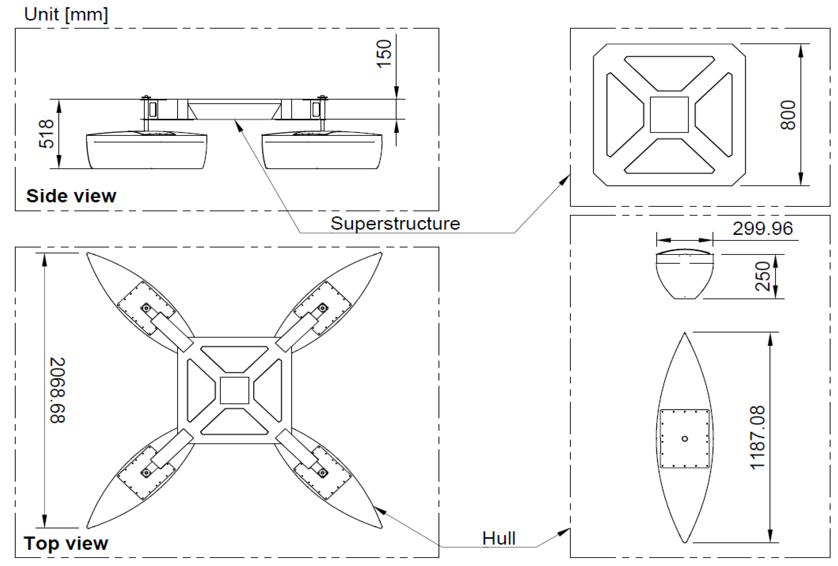
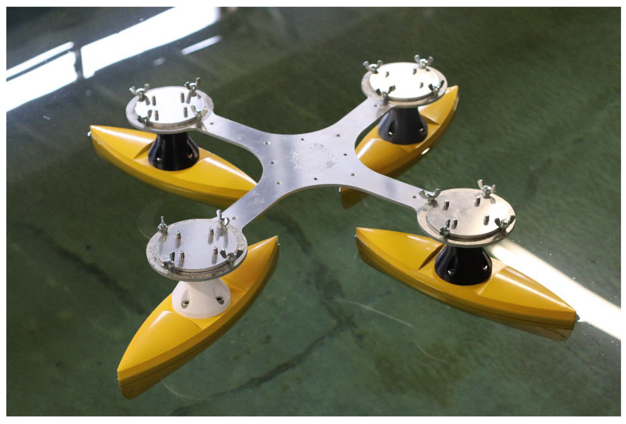
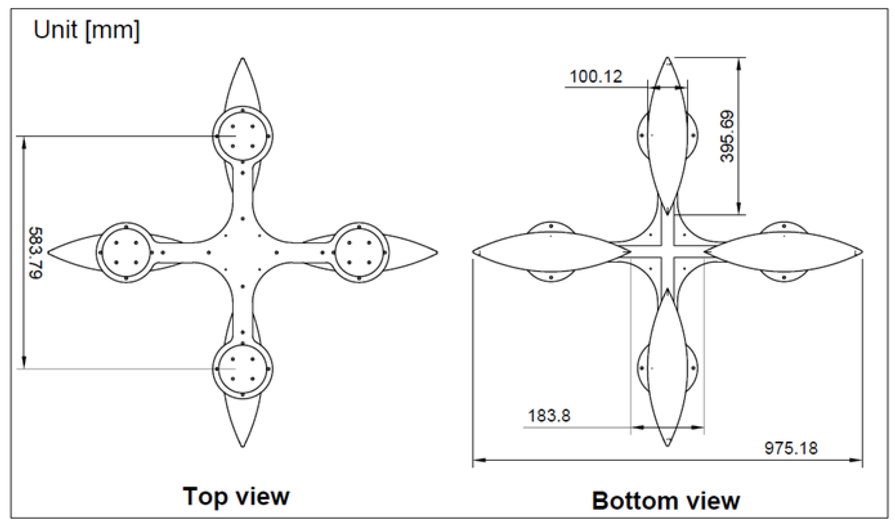
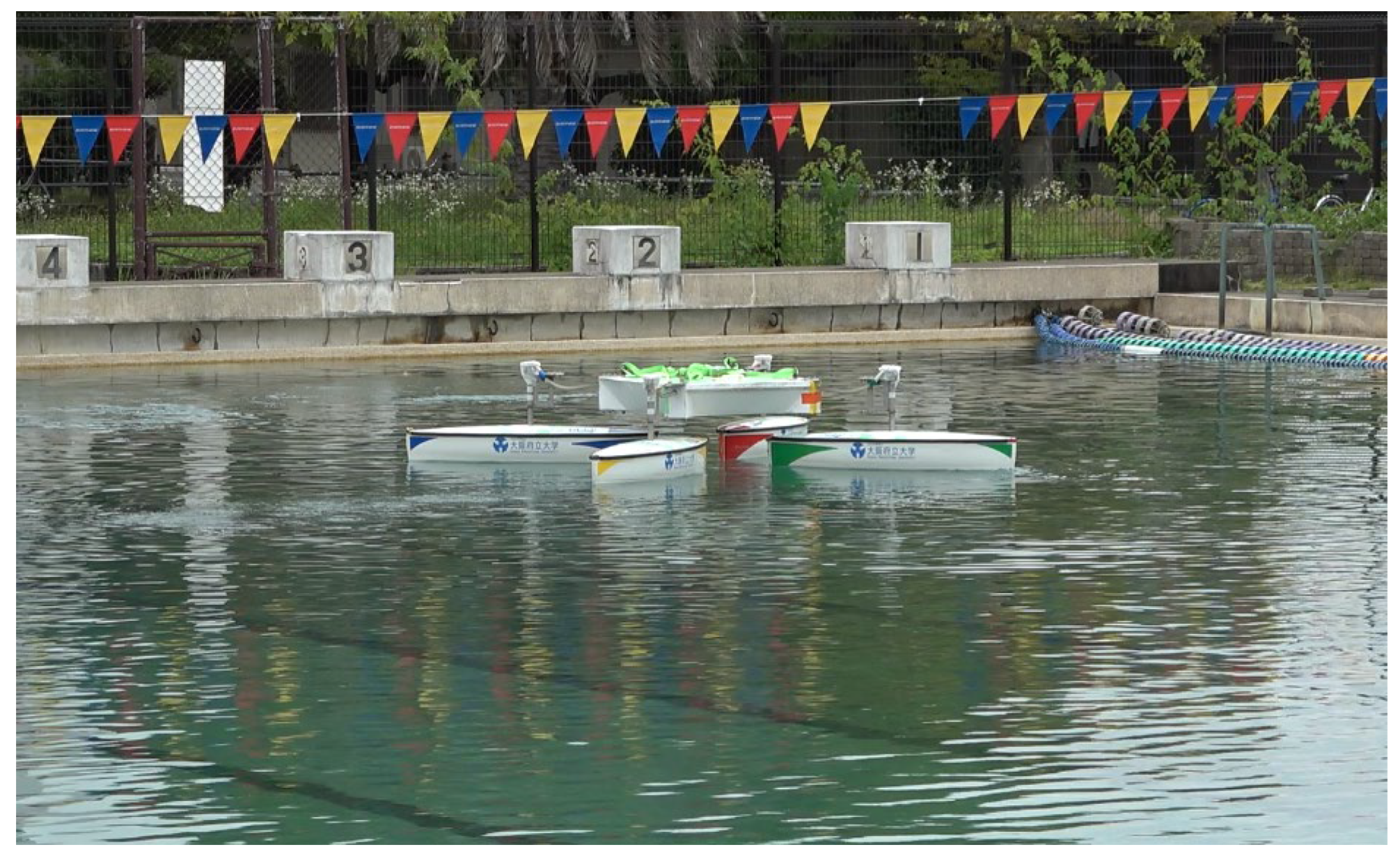
2.2. 1/3 Scale Experiment Model

To perform a simulation with high accuracy, we conducted tank tests on a 1/3 scale model. The scaled model built is shown in Figure 4, and primary dimensional drawings are as shown in Figure 5.

3. Mathematical Model

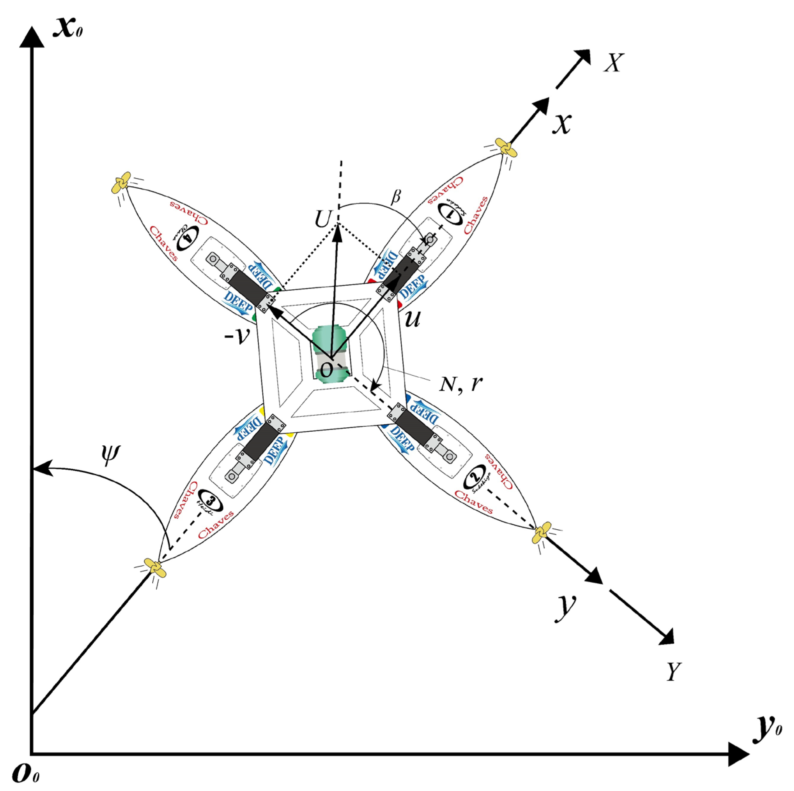
3.1. Motion Equations

Figure 6 shows the defined coordinate system of the vessel. The space-fixed coordinate system o₀-x₀y₀ was firstly defined. The x₀-y₀ plane was aligned with the hydrostatic surface, and the yaw angle ψ concerning the x₀ axis was defined. The coordinate system o-xy was then defined for the vessel body. On the horizontal plane, the midship and center of vessel gravity overlap with the geometric features of the vessel. In this study, since only the horizontal movement of the vessel was considered, it was feasible to align the origin of the coordinate system, as it was fixed to the vessel body along with the position of the center of gravity of the vessel. The x-axis direction on the No.1 hull side was set, and the y-axis was placed laterally. The x-y plane was also parallel to the hydrostatic surface.

Table 2. Significance of symbols.

X	Hydrodynamic force in the x-axis [N]
Y	Hydrodynamic force in the y-axis [N]
N	Hydrodynamic moment around the z-axis [Nm]
U	Forward movement speed [m/s]
u	Velocity in the x-axis [m/s]
v	Velocity in the y-axis [m/s]
r	Yaw rate [rad/s]
β	Drift angle [deg.]
ψ	Heading angle [deg.]

shows the significance of the symbols used in this coordinate system.

This study adopts the MMG (Maneuvering Modeling Groupe) as the mathematical model [18]. Considering the coordinate system that moves with the vessel body (o-xy), the motion equations are as shown below:

$$\left\{\begin{array}{c}\left(m+m_x\right)\dot{u}-\left(m+m_{\mathrm{y}}\right)vr=X\\ \left(m+m_y\right)\dot{v}+\left(m+m_x\right)ur=Y\\ (I_{\mathrm{zz}}+J_{\mathrm{zz}})\dot{r}=N\end{array}\right.$$

(1)

where m: mass of vessel; m_x: added mass in the x-axis; m_y: added mass in the y-axis;

I_zz: the moment of inertia around the center of gravity;

J_zz: the added moment of inertia around the center of gravity;

r: yaw rate; u: velocity in the x-axis; and v: velocity in the y-axis.

X, Y, and N are the forces acting on the vessel body other than the additional mass component. Specifically, the forces acting on the vessel body can be written as shown in Equation (2).

$$\left\{\begin{array}{c}X=X_H+X_P+X_E\\ Y=Y_H+Y_P+Y_E\\ N=N_H+N_E\end{array}\right.$$

(2)

X_H, Y_H, and N_H are forces acting on the four hulls generated from water. X_P and Y_P are the thrusts of the propellers. X_E, Y_E, and N_E are other external force components, mainly wind load. This paper ignores the effect of waves and the water current since aquaculture farms are usually in calm waters.

According to the test results conducted in calm water, we discovered that the parallel motion of vessel drifting during DP is slow (generally about 0.25 m/s), and the yawing rate is consistently less than 0.026 rad/s. Hence, as shown in Equation (3), the forces acting on the hulls due to parallel and static turning motions are only considered based on the quasi-static assumption in this study. We will investigate X_H(u,v,0), Y_H(u,v,0) and N_H(u,v,0) by conducting the oblique towing tests, and N_H(0,0,r) by the static turning tests.

$$\left\{\begin{array}{c}{X}_H=X_{H\left(u, v, 0\right)}\\ Y_H=Y_{H\left(u, v, 0\right)}\\ N_H=N_{H\left(u, v, 0\right)}+N_{H\left(0, 0, r\right)}\end{array}\right.$$

(3)

In addition, the Quadmaran vessel maintains front-back and left-right symmetry while in DP. The principal terms of additional mass and moment inertia (m_x, m_y, J_zz in Equation (1)) are considered sufficient in this study. Here, m_x = m_y since the movements in the x and y directions are happening to similar extents while in DP.

Equation (1) is used to predict the maneuvering motion. The direction (ψ) and position (x₀, y₀) of the vessel in space are also essential information. Equation (4) is also considered along with Equation (1).

$$\left\{\begin{array}{c}\dot{x_0}=u\cos \psi -v\sin \psi \\ \dot{y_0}=u\sin \psi +v\cos \psi \\ \dot{\psi }=r\end{array}\right.$$

(4)

Next, the forces acting on the hulls, the thrust of the propeller, and the wind load on the superstructure and hulls individually will be explained.

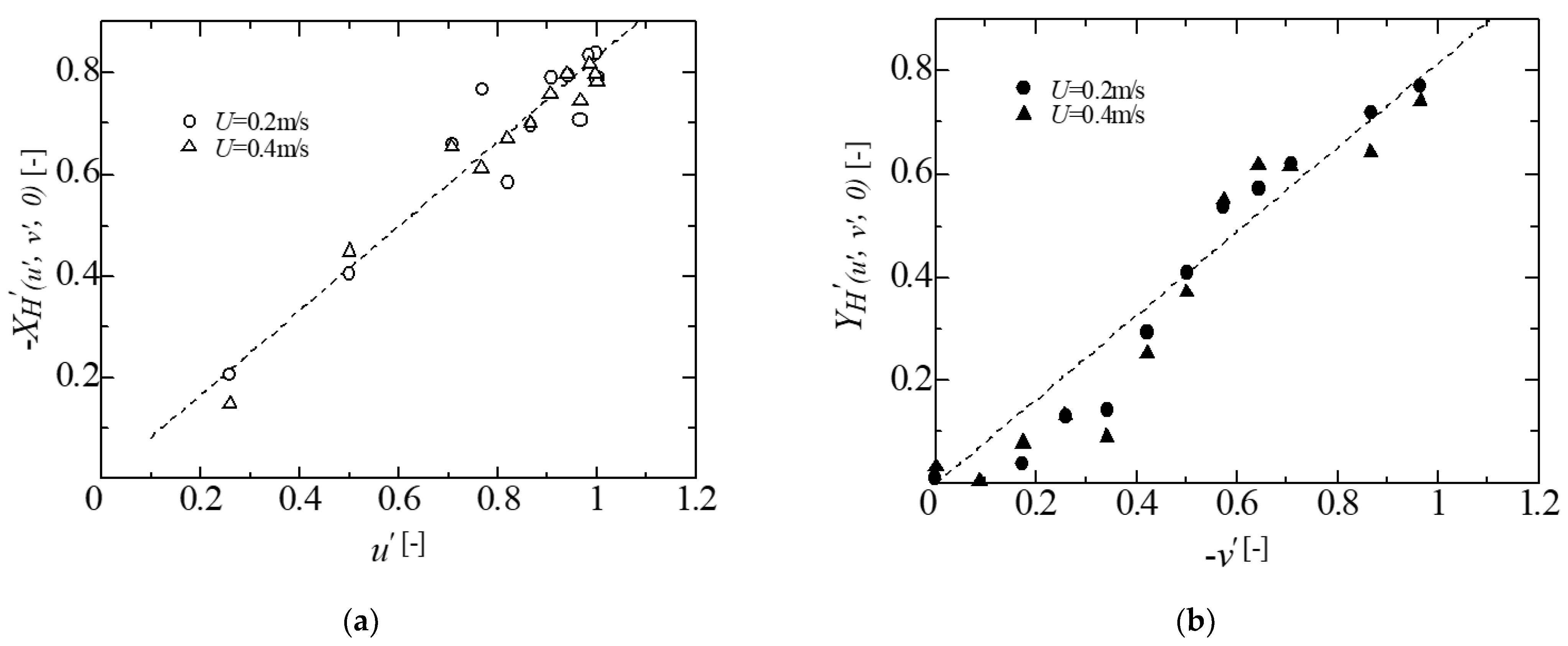
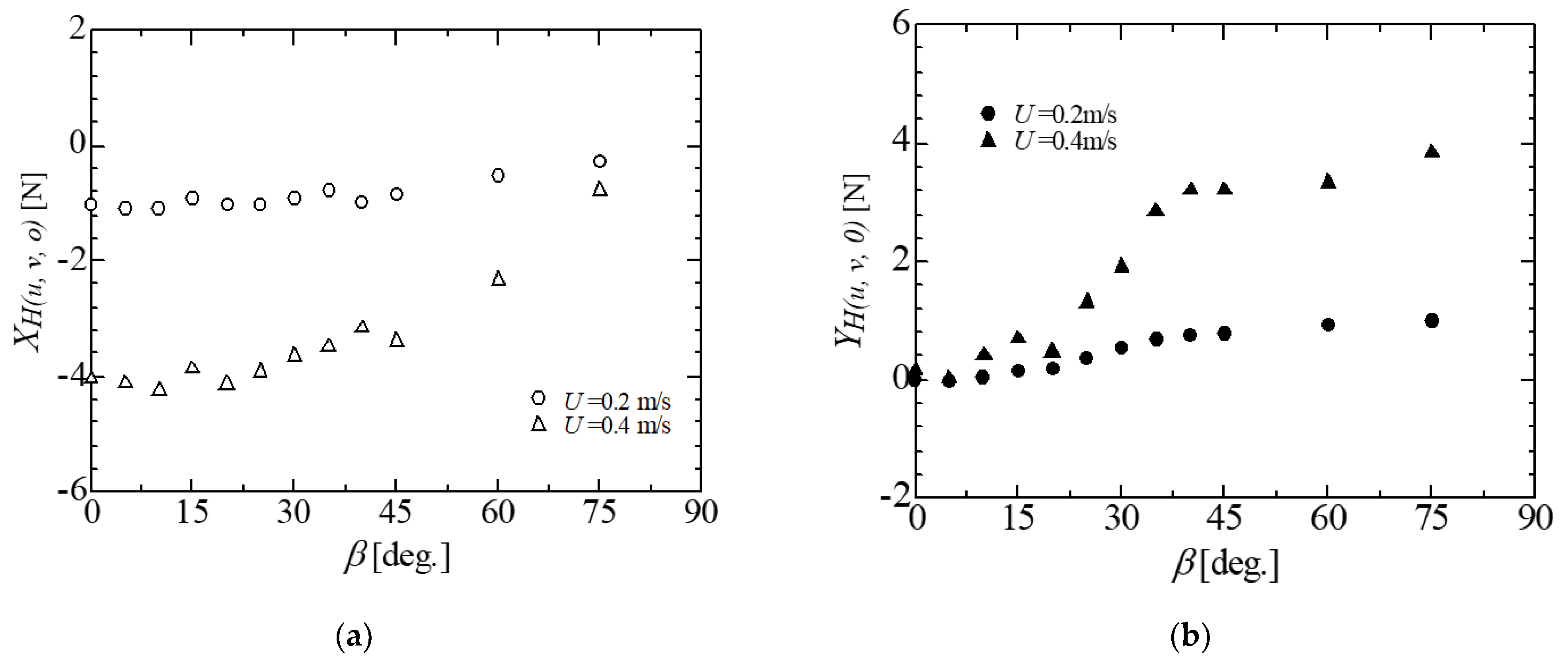
3.2. Water Loads Generated from Parallel Motion

We surveyed the water loads acting on the four hulls in the x and y-axis, and the moment around the z-axis due to parallel motion by conducting oblique towing tests using the 1/3 scaled model. Equation (5) expresses X_H, Y_H, and N_H.

$$\left\{\begin{array}{c}{X}_{H\left(u, v, 0\right)}=\frac{1}{2}\rho Ld{U}^2{X}_H^{\prime }\left(u^{\prime }, v^{\prime }, 0\right)\\ Y_{H\left(u, v, 0\right)}=\frac{1}{2}\rho Ld{U}^2{Y}_H^{\prime }\left(u^{\prime }, v^{\prime }, 0\right)\\ N_{H\left(u, v, 0\right)}=\frac{1}{2}\rho L^{2}d{U}^2{N}_H^{\prime }\left(u^{\prime }, v^{\prime }, 0\right)\end{array}\right.$$

(5)

Here ρ is the density of water, and L is the representative length of the vessel (the diagonal length while in the DP configuration, Figure 5). d is the planned draft, and U is the advanced speed defined as $U\equiv \sqrt{u^2+v^2}$. $X_H^{\prime }$, $Y_H^{\prime }$, and $N_H^{\prime }$, which correspond to the hydrodynamic derivatives, “′” means a dimensionless value. In this study, these hydrodynamic derivatives were considered functions of the dimensionless surge (u′) and sway (v′) velocities.

Since these forces vary based on the drift angle, the fluid force was measured in the oblique towing test at two towing speeds for a range of drift angles. Figure 7 shows the tank test setup, and

Table 3. Oblique towing test conditions.

Item	Value	Unit
Towing speed (U)	0.2, 0.4	m/s
Drift angle (β)	0, 5, 10, 15, 20, 25, 30, 35, 40, 45, 60, 75	deg.

outlines the test conditions.

Figure 8 shows the forces acting on the hulls in x and y directions in various towing speeds and drift angles. From the measurement results on the x-axis, as the drift angle increased, the force decreased. Moreover, after 45 degrees, the deceleration slowed down significantly. An apparent sudden increase was confirmed around 15 and 45 degrees. Contrary to the x-axis, the measured force on the y-axis gradually increased with the drift angle, and slowed down after 45 degrees. Similarly, a sudden decrease occurred around 15 and 45 degrees. It can be concluded that a particular hull configuration determined the fluid force acting on the vessel.

Furthermore, when the dimensionless forces and velocities are considered:

$$X_H^{\prime }, Y_H^{\prime }=X_H, X_H/\frac{1}{2}\rho Ld{U}^2, u^{\prime }, v^{\prime },=u, v/U$$

(6)

Figure 9 shows the dimensionless forces as the vertical axis and u’, v’ as the horizontal axis. The dotted line approximates the linear relationship, which sufficiently outlines the experimental results. We treat the line slope as the hydrodynamic derivatives by the least-square method.

The moment due to parallel motion was thought to be generated. Figure 10a shows the measurement results of the moment in the oblique towing test. It can be clearly seen that the moment fluctuated wildly at a drift angle between 20 and 45 degrees, and peaked at a maximum of around 35 degrees. Also, when the moment was set as dimensionless, we used the following equation:

$$N_H^{\prime }=\frac{N_H}{\frac{1}{2}\rho L^{2}d{U}^2}$$

(7)

Here we use the dimensionless velocity component v’ as the horizontal axis, and Figure 10b shows their relationship. The dimensionless moments have the same trends and roughly the same value at a v′ independent of advancing speed. The dotted line is a cubic curve approximation based on the value of practical velocity (U = 0.2 m/s). It has been used to calculate the part of the moment generated from parallel motion.

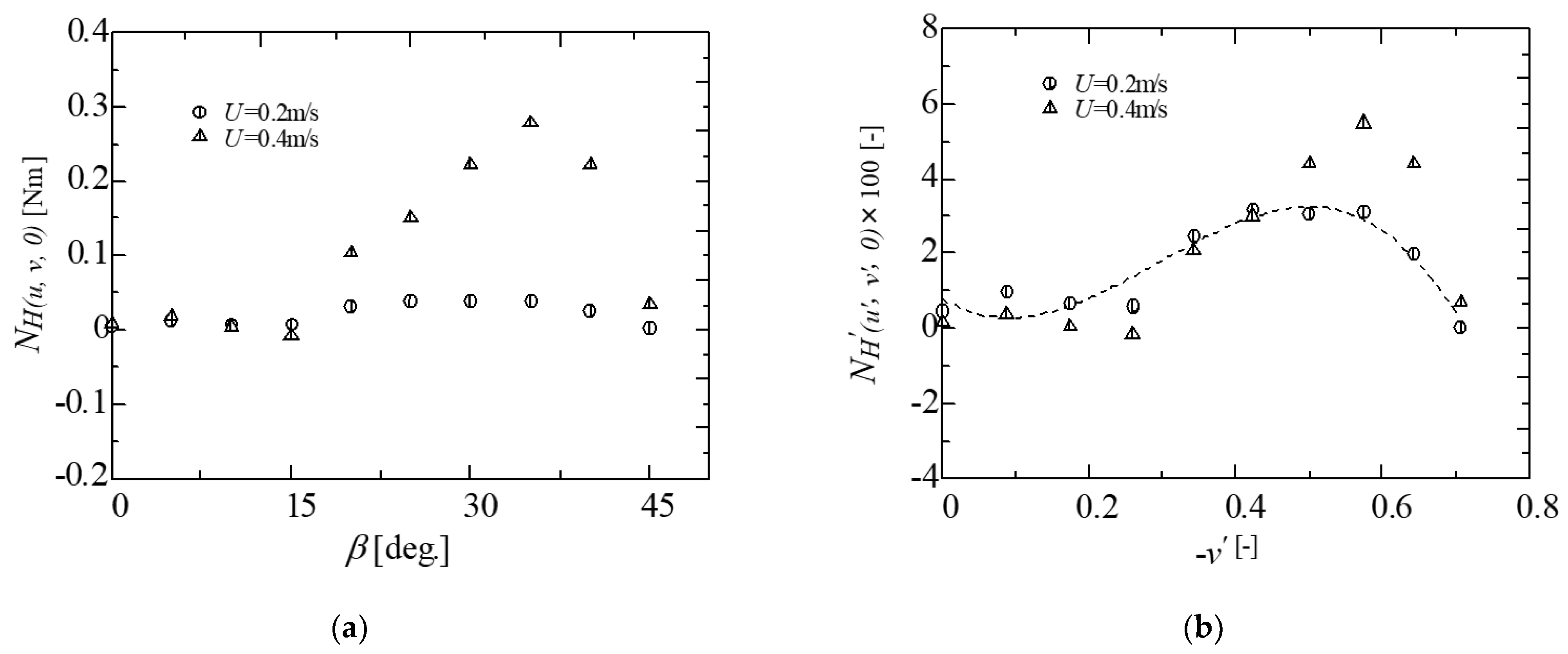
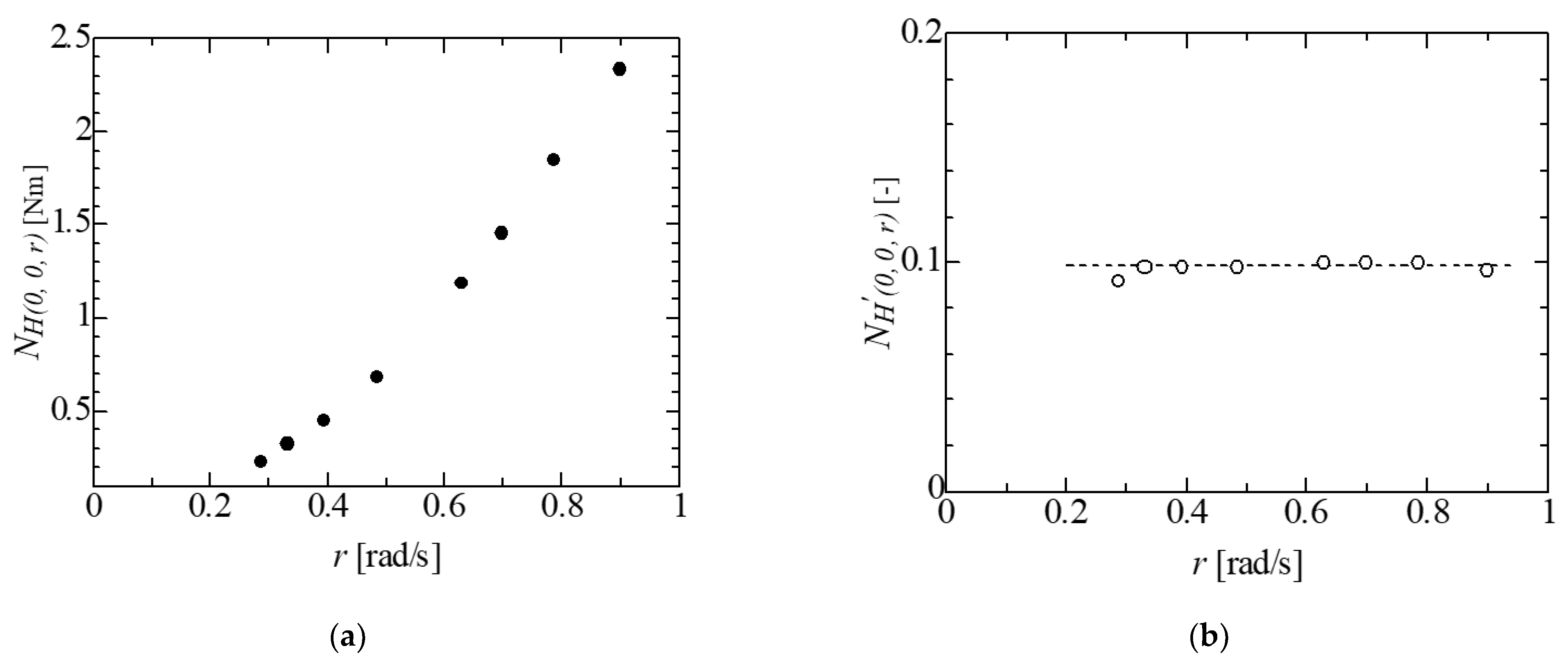
3.3. Moment Generated from Static Yawing Motion

The moment due to the static yawing motion was also considered, and examined by rotating the model at a constant yaw rate (r) using a turning motor. The moment measured at different yaw rates is shown in Figure 11a. The results demonstrated that the moments were proportional to the square of the yaw rate. This suggests that we can obtain the yaw moment coefficient (N_H^’_(0,0,r)) of constant value at any yaw rate. The yaw moment coefficient was obtained as in Equation (8). Figure 11b shows the relationship between the yaw moment coefficient and the yaw rate relationship. We can see that the coefficients were irrelevant to the yaw rate and matched well at roughly 0.1.

$$N_{H\left(0, 0, r\right)}^{\prime }=\frac{N_{H\left(0,0,r\right)}}{\frac{1}{2}\rho r^2{L}^{4}d}$$

(8)

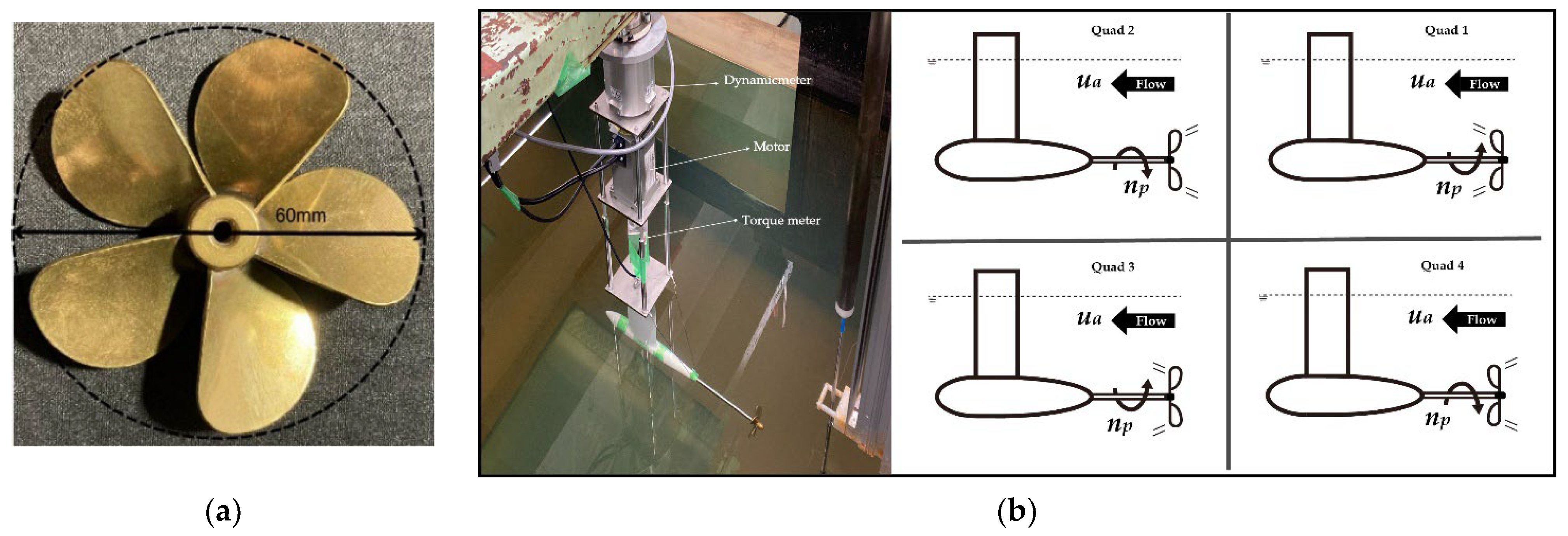
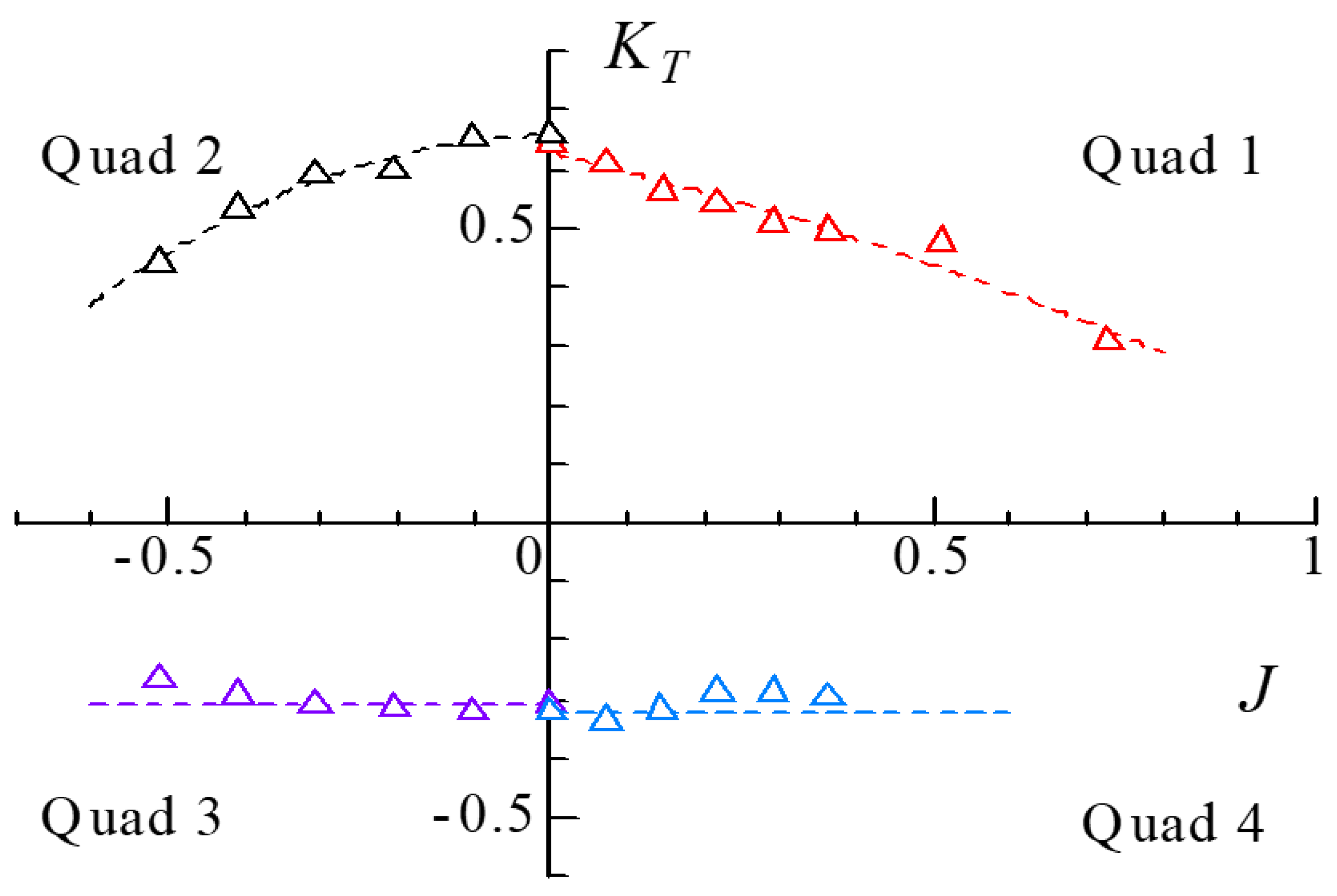
3.4. Propeller Thrust

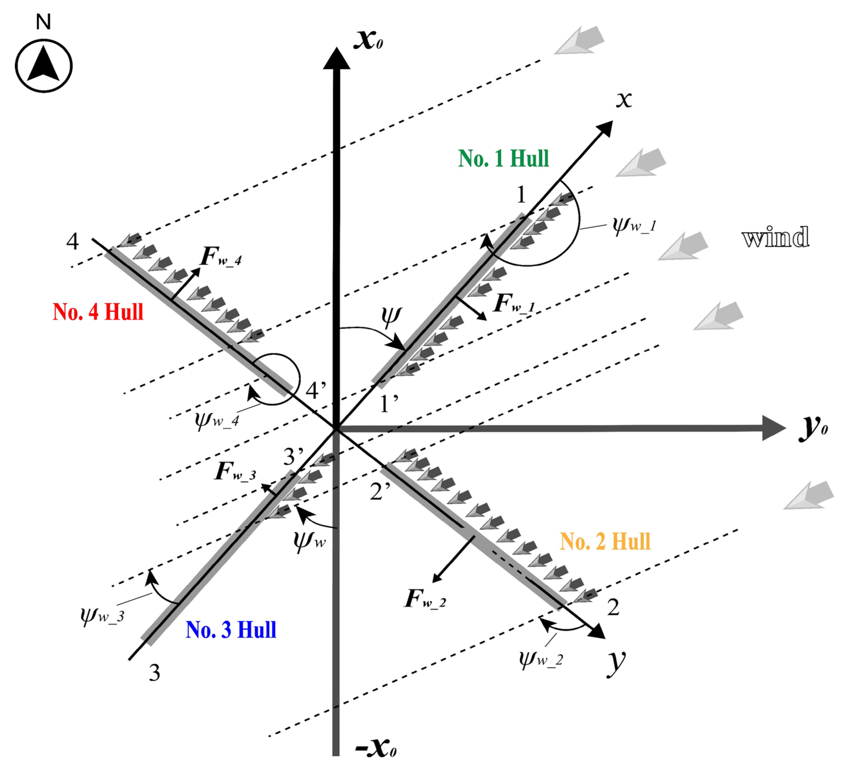
The Quadmaran vessel was equipped with four propellers as shown in Figure 12a: one for each hull. X_P and Y_P as shown in Equation (2) were the resultant propeller thrusts along the x and y-axis. From Figure 6, we can see that X_P was the resultant thrust force of propellers No. 1 and 3, while Y_P was the resultant thrust force of propellers No. 2 and 4. For each propeller, the thrust was generally positively correlated with water density, rotational speed, and operating area. Equation (9) is adopted to express the thrust for the propeller in this study [19].

$$T_P=\left(1-t\right)K_T\rho n_P^2{D}_P^4$$

(9)

Here, t is the thrust deduction coefficient, ρ is the water density, n_P is the rotational speed, D_P is the diameter of the propeller, K_T is the thrust coefficient, which is represented as a function of the advance ratio J, with J being defined as follows:

$$J=\frac{\left(1-w_p\right)V_a}{n_P{D}_P}$$

(10)

V_a is the speed for each hull. W_p is the effective wake fraction factor, which is a coefficient representing the decrease in the flow velocity near the propeller due to the effect of the forward hull. The value measured through the wake fraction measurement test conducted by Kamio et al. has been used [7].

In regards to the thrust deduction coefficient (t in Equation (9)), since the navigation speed while in DP is slow, the increase in hull resistance due to the operation of the propeller can be ignored. It is appropriate to treat the thrust deduction coefficient as 0 based on the results of the test of the thrust deduction coefficient.

The thrust coefficients (K_T) were surveyed using a Propeller Open Test (POT). The rotation speed, rotation direction, and traveling direction of four propellers were constantly changing depending on the vessel’s traveling state while in DP. Therefore, it was necessary to understand the characteristics of the propeller in all four quadrants. The POT was thus conducted in the circulating water tank as shown in Figure 12b. The test conditions considered were that the propeller rotation was in a clockwise and a counterclockwise direction, and the hull was traveling in headway and sternway directions. Since the water in the circulating water tank could only flow in one direction, we changed the configuration direction of the propeller as an alternative.

Table 4. Propeller Open Test conditions.

Item	Value	Unit
Flow velocity (ua)	0.0, 0.1, 0.2, 0.4, 0.5, 0.7, 1.0 (0.7, 1.0 only for Quad 1)	m/s
Rotational speed (np)	976	rpm

shows the POT conditions.

The change of K_T is the independent performance curve of the propeller. As shown in Figure 13, especially in Quad 1 and Quad 2, K_T tended to be smaller as J (absolute value) increased. The curve of Quad 3 and Quad 4 was much smoother when the propeller reversed. This study used the thrust coefficient at the advance ratio J = 0 for Quad 3 and 4, as proposed by Hewins et al. [20].

K_T is expressed as a function of J, as shown in the following equation:

$$K_T=k_0+k_{1}J+k_2{J}^2$$

(11)

Here, k₀, k₁, and k₂ are coefficients representing the characteristics of K_T based on the measurement data.

3.5. Wind Loads

The external force due to wind is less of a concern compared to water resistance, and is often neglected during DP. However, it should not be neglected if the vessel has a bigger superstructure. This particular Quadmaran vessel had four hulls and a superstructure on which the control board and batteries were loaded. In addition, it was also found from the actual sea sailing tests that the wind effect was evident. Hence, we modeled the forces acting on the Quadmaran vessel (including the four hulls and the superstructure) generated from wind using the database of wind load tests [21]. The moment acting on the superstructure was ignored, as the simple shape was previously found from the wind load test results. Although, for hulls, the wind load test was conducted in a single hull because of the equipment limitations. The following model simulated the forces, including the moment, considering the interaction between hulls.

Figure 14 shows the coordinate system for modelling wind loads. For simplicity, each hull was assumed to be a flat board, and the origin of the vessel coincided with origin of the space-fixed coordinate system (o₀-x₀y₀). The orientation of each hull facing the wind had a significant effect on the wind load received by each hull, and could not be modelled in a straightforward way. Therefore, in this study, we developed a model such that the wind load received by each hull could be considered. The wind direction angle, ${\psi }_w$ (w means wind) is defined as the relative angle between each hull of the vessel and the streamline of the wind based on a clockwise convention. Further, ${\psi }_{w\_i}$ (i = 1, 2, 3, 4) for each hull can be defined as shown in Figure 14. Correspondingly, $F_{w\_i}$ (i = 1, 2, 3, 4) are the forces that each hull receives from the wind in the out of plane direction (positive force as per left hand rule). The in-plane wind force acting on the hull was small and negligible. Symbols 1~4 and 1′~4′ represent the position of the stern and bow of the No. 1~4 hulls, respectively.

The force experienced by each hull is proportional to the effective length ($l_{w\_i}$, i = 1, 2, 3, 4) of the hull facing the wind stream. Therefore, it is necessary to obtain these effective lengths based on the relative orientation of each hull and wind direction, including the wind blocked by the upstream hulls. The wind force is considered to act at the center of the effective length for each hull. As Figure 14 shows, it can be understood that the effective length of each hull varied with the relative angle of the hull orientation and streaming wind. In the case of Figure 14, we can understand that $l_{w\_1}=L$, $l_{w\_2}=L$, however, $l_{w\_3}$, and $l_{w\_4}$ were shorter than L affected by hull No. 1 and 2 (the effective wind received on hull No. 3 and 4 was reduced). The details of effective length of each hull hit by the wind are summarized as shown in Equation (12). If ${\psi }_w<\psi$, ${\psi }_w$ will be handled as ${\psi }_w+360°$.

$$\begin{array}{cc}{l}_{w\_1}=\left\{\begin{array}{c}0,{\psi }_w-\psi =0^{\circ }\\ L,0^{\circ }<{\psi }_w-\psi <{45}^{\circ }\\ L,{45}^{\circ }\le {\psi }_w-\psi <{90}^{\circ }\\ L,{\psi }_w-\psi ={90}^{\circ }\\ (L+l)\left(1-\frac{1}{\left|tan\left({\psi }_w-\psi \right)\right|}\right),{90}^{\circ }<{\psi }_w-\psi <{135}^{\circ }\\ l\left(\frac{1}{\left|tan\left({\psi }_w-\psi \right)\right|}-1\right),{135}^{\circ }\le {\psi }_w-\psi <{180}^{\circ }\\ 0,{\psi }_w-\psi ={180}^{\circ }\\ l\left(\frac{1}{\left|tan\left({\psi }_w-\psi \right)\right|}-1\right),{180}^{\circ }<{\psi }_w-\psi <{225}^{\circ }\\ (L+l)\left(1-\frac{1}{\left|tan\left({\psi }_w-{\psi }^{\prime }\right)\right|}\right),{225}^{\circ }\le {\psi }_w-\psi <{270}^{\circ }\\ L,{\psi }_w-\psi ={270}^{\circ }\\ L,{270}^{\circ }<{\psi }_w-\psi <{315}^{\circ }\\ L,{315}^{\circ }\le {\psi }_w-\psi <{360}^{\circ }\end{array}\right.& l_{w\_3}=\left\{\begin{array}{c}0,{\psi }_w-\psi =0^{\circ }\\ l\left(\frac{1}{\left|tan\left({\psi }_w-\psi \right)\right|}-1\right),0^{\circ }<{\psi }_w-\psi <{45}^{\circ }\\ (L+l)\left(1-\frac{1}{\left|tan\left({\psi }_w-\psi \right)\right|}\right),{45}^{\circ }\le {\psi }_w-\psi <{90}^{\circ }\\ L,{\psi }_w-\psi ={90}^{\circ }\\ L,{90}^{\circ }<{\psi }_w-\psi <{135}^{\circ }\\ L,{135}^{\circ }\le {\psi }_w-\psi <{180}^{\circ }\\ 0,{\psi }_w-\psi ={180}^{\circ }\\ L,{180}^{\circ }<{\psi }_w-\psi <{225}^{\circ }\\ L,{225}^{\circ }\le {\psi }_w-\psi <{270}^{\circ }\\ L,{\psi }_w-\psi ={270}^{\circ }\\ (L+l)\left(1-\frac{1}{\left|tan\left({\psi }_w-\psi \right)\right|}\right),{270}^{\circ }<{\psi }_w-\psi <{315}^{\circ }\\ l\left(\frac{1}{ltan\left({\psi }_w-\psi \right)\mid }-1\right),{315}^{\circ }\le {\psi }_w-\psi <{360}^{\circ }\end{array}\right.\\ l_{w\_2}=\left\{\begin{array}{c}L,{\psi }_w-\psi =0^{\circ }\\ L,0^{\circ }<{\psi }_w-\psi <{45}^{\circ }\\ L,{45}^{\circ }\le {\psi }_w-\psi <{90}^{\circ }\\ 0,{\psi }_w-\psi ={90}^{\circ }\\ L,{90}^{\circ }<{\psi }_w-\psi <{135}^{\circ }\\ L,{135}^{\circ }\le {\psi }_w-\psi <{180}^{\circ }\\ L,{\psi }_w-\psi ={180}^{\circ }\\ (L+l)\left(1-\left|tan\left({\psi }_w-\psi \right)\right|\right),{180}^{\circ }<{\psi }_w-\psi <{225}^{\circ }\\ l\left(\left|tan\left({\psi }_w-\psi \right)\right|-1\right),{225}^{\circ }\le {\psi }_w-\psi <{270}^{\circ }\\ 0,{\psi }_w-\psi ={270}^{\circ }\\ l\left(\left|tan\left({\psi }_w-\psi \right)\right|-1\right),{270}^{\circ }<{\psi }_w-\psi <{315}^{\circ }\\ (L+l)\left(1-\left|tan\left({\psi }_w-\psi \right)\right|\right),{315}^{\circ }\le {\psi }_w-\psi <{360}^{\circ }\end{array}\right.& l_{w\_4}=\left\{\begin{array}{c}L,{\psi }_w-\psi =0^{\circ }\\ (L+l)\left(1-\left|tan\left({\psi }_w-\psi \right)\right|\right),0^{\circ }<{\psi }_w-\psi <{45}^{\circ }\\ l\left(\left|tan\left({\psi }_w-\psi \right)\right|-1\right),{45}^{\circ }\le {\psi }_w-\psi <{90}^{\circ }\\ 0,{\psi }_w-\psi ={90}^{\circ }\\ l\left(\left|tan\left({\psi }_w-\psi \right)\right|-1\right),{90}^{\circ }<{\psi }_w-\psi <{135}^{\circ }\\ (L+l)\left(1-\left|tan\left({\psi }_w-\psi \right)\right|\right),{135}^{\circ }\le {\psi }_w-\psi <{180}^{\circ }\\ L,{\psi }_w-\psi ={180}^{\circ }\\ L,{180}^{\circ }<{\psi }_w-\psi <{225}^{\circ }\\ L,{225}^{\circ }\le {\psi }_w-\psi <{270}^{\circ }\\ 0,{\psi }_w-\psi ={270}^{\circ }\\ L,{270}^{\circ }<{\psi }_w-\psi <{315}^{\circ }\\ L,{315}^{\circ }\le {\psi }_w-\psi <{360}^{\circ }\end{array}\right.\end{array}$$

(12)

The relative hull orientation ${\psi }_{w\_i}$ is defined by the formula below:

$${\psi }_{w\_i}=\left[\begin{array}{c}{\psi }_w+180°-\psi \\ {\psi }_w+90°-\psi \\ {\psi }_w-\psi \\ {\psi }_w-90°-\psi \end{array}\right]$$

(13)

Equation (14) expresses the force generated on each hull perpendicular to the hull based on the above model and wind load test results [22].

$$F_{w\_i}=0.64\frac{l_{w\_i}}{L}\sin {\psi }_{w\_i}$$

(14)

Therefore, for the coordinate system fixed to the vessel body, the forces, including hulls and the superstructure ($F_{wx\_s}$, $F_{wy\_s}$) on the x and y-axis, become

$$X_E=F_{w\_4}-F_{w\_2}+F_{wx-s}$$

(15)

$$Y_E=F_{w\_1}-F_{w\_3}+F_{wy-s}$$

(16)

As mentioned earlier, the force acts at the center of the effective length for each hull. If lever arm length, $l_{w\_arm\_i}$ of each hull is defined, yaw moment due to wind can be obtained as shown in Equation (17).

$$N_E={\displaystyle \sum }_{i=1}^4{F}_{w\_i}{l}_{w\_arm\_i}$$

(17)

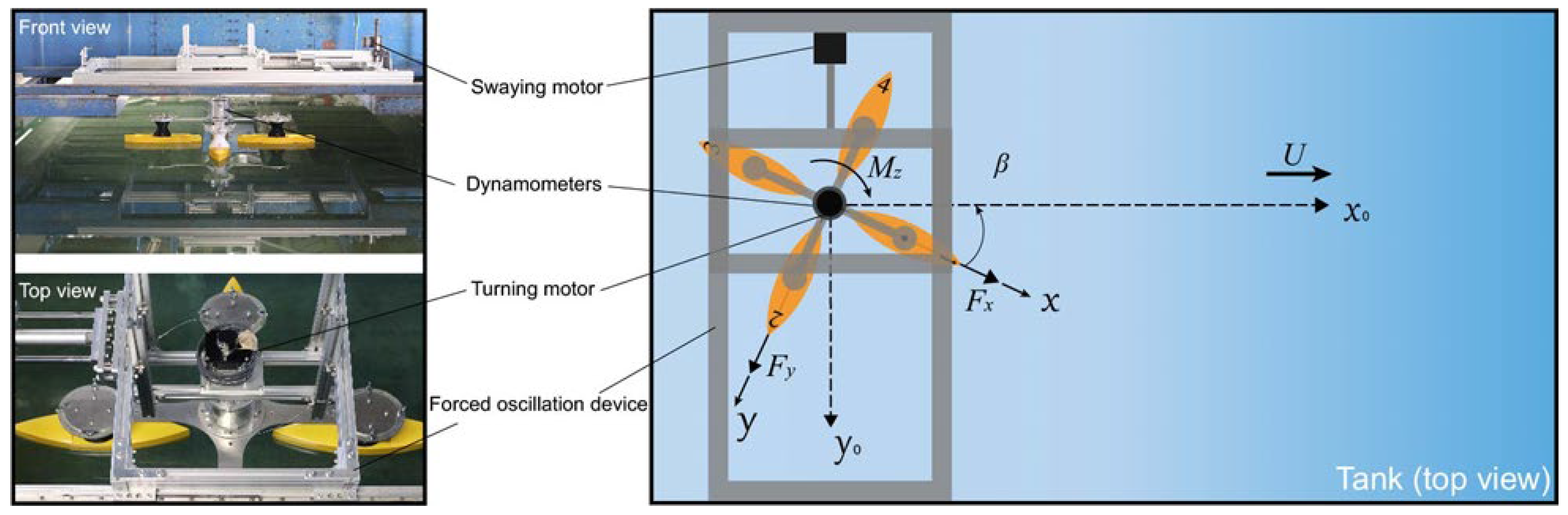
4. Experimental Validation

In this section, the results of the computational model were compared with the experimental results, and a computational model was developed, verified, and validated. Firstly, the computational model was verified with tests conducted in the swimming pool (a calm water area) of Osaka Metropolitan University, Osaka, Japan. Secondly, we compared the predicted results of the DP computational model with the actual sea test conducted at Nanao Bay, Ishikawa, Japan.

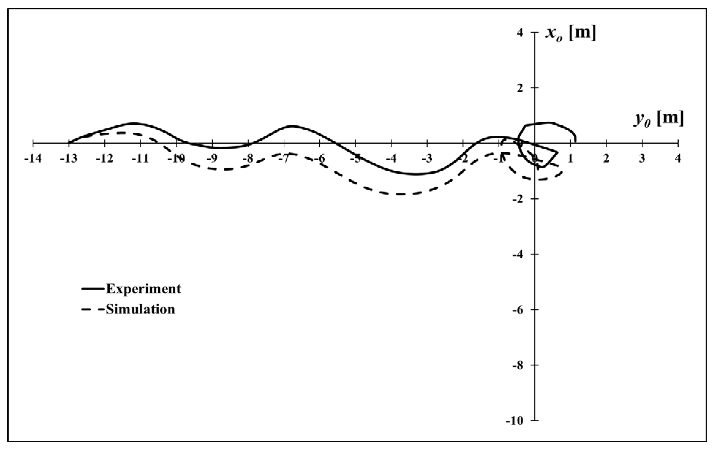
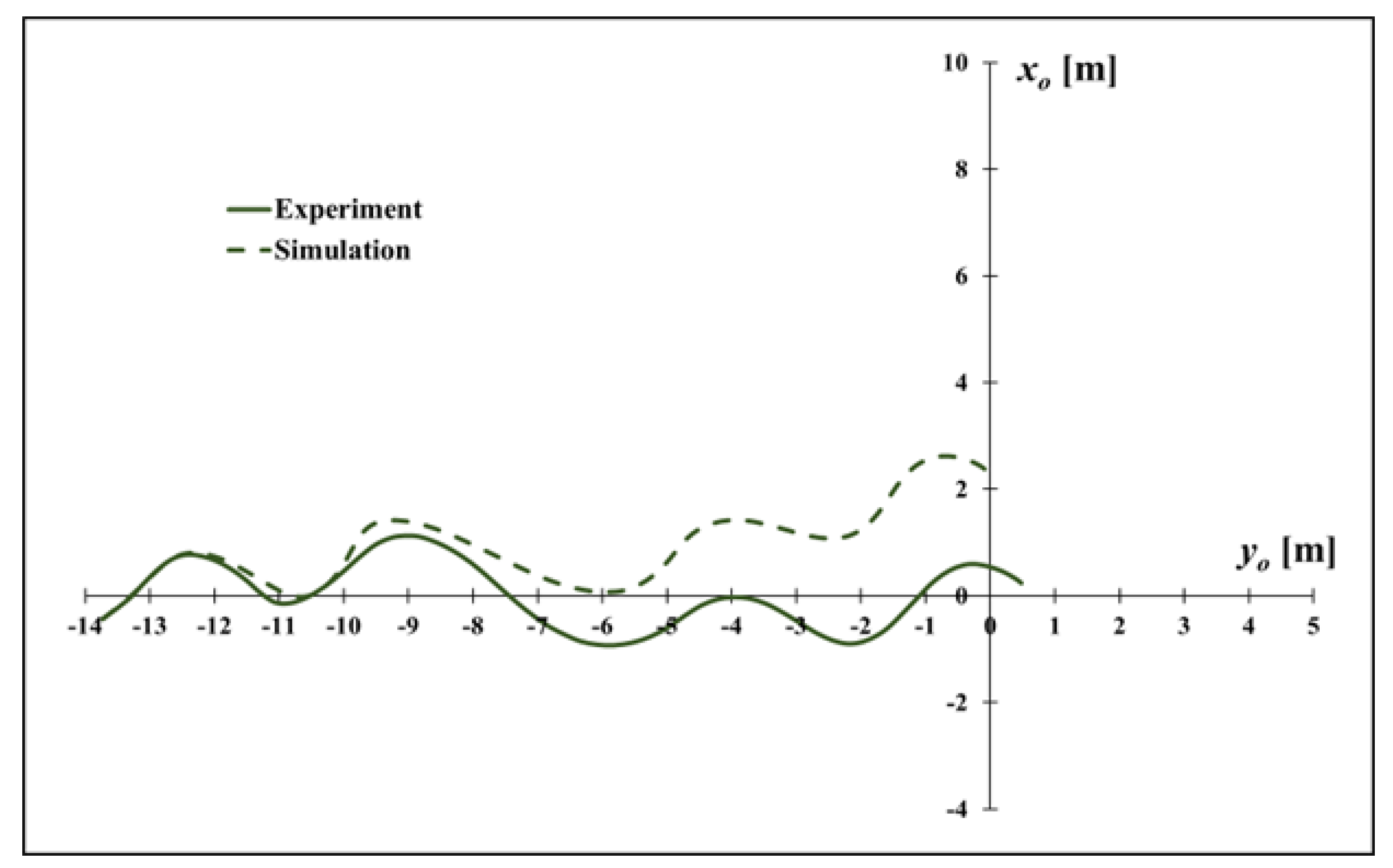
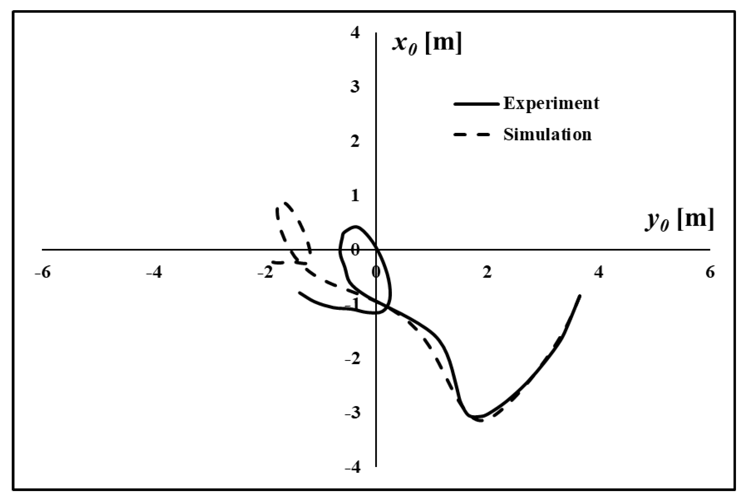
4.1. Calm Water Area

The validation in calm water was conducted by navigating the Quadmaran vessel automatically in a DP posture using various initial conditions of position and heading angle. The GPS system, ichimill, recorded the location information every 2 s [23], and was confirmed to be accurate with an error within centimeters through tests. In addition, the recorded rotation speed value of the four propellers was used in the calculation. Moreover, in this study, to avoid machine time delays and accurately grasp the direction of rotation of the propeller, we decided to operate the propellers only in the forward direction. In the tests, out of the four propellers, we only operated the two that rotate in the forward direction.

Figure 15 shows the running test scene in the pool while in DP. The wind was weak on the test day and was ignored. Figure 16 shows the recorded DP trajectories of the Quadmaran vessel in the calm water area with the heading angle set to 0, 45, and 90 degrees from a specific starting position with no initial speed and yaw rate. From the recorded DP trajectory, we can see that the Quadmaran vessel navigated to the designated reference point, no matter the initial heading angle. Moreover, after arriving at the target, it remained within roughly 1 m of the designated reference point.

Here, we employed the developed motion prediction model and compared it with the calm water experiment results. Figure 17, Figure 18 and Figure 19 compare the experiment and simulation results when the initial heading angle was 0, 45, and 90 degrees. From the results, we can see that the model predicted the motion of a Quadmaran vessel during DP with an accuracy of roughly 2 m. However, the trajectory of the path of the vessel was different and varied depending on the initial heading angle and loads acting on the vessel. Especially in the case of an initial heading of 45 degrees (Figure 18), the trajectory demonstrated the effect of moment generated due to parallel motion. As discussed previously in Figure 10a, moment generated fluctuated between 20 and 45 degrees, and it was relatively challenging to predict the motion while in DP. The error in position prediction could be further reduced if the moment generated in parallel motion can be accurately assessed. Propeller deformation due to long-term use and GPS error are other sources of error in prediction for all the simulations. However, for practical purposes, an accuracy of 2 m is small, and it can be said that the developed computational model predicted the trajectory motion very well.

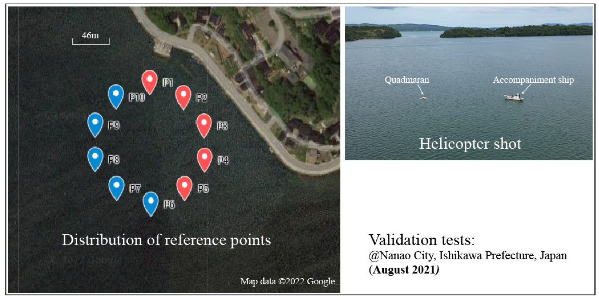
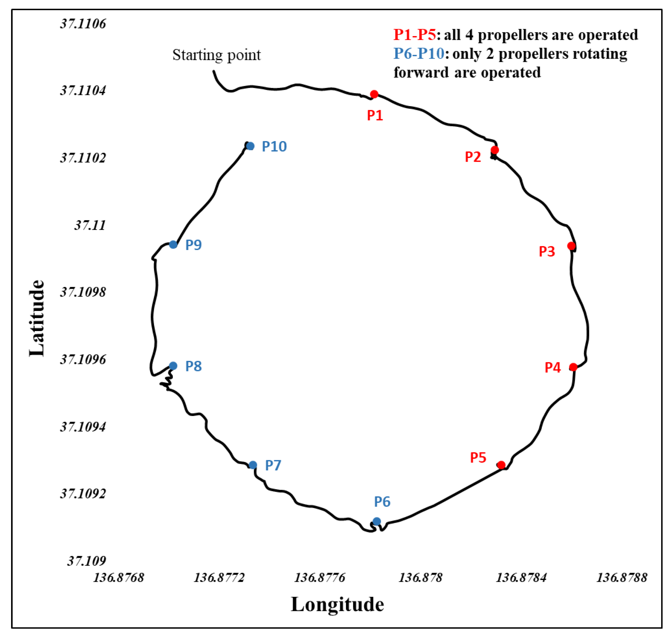
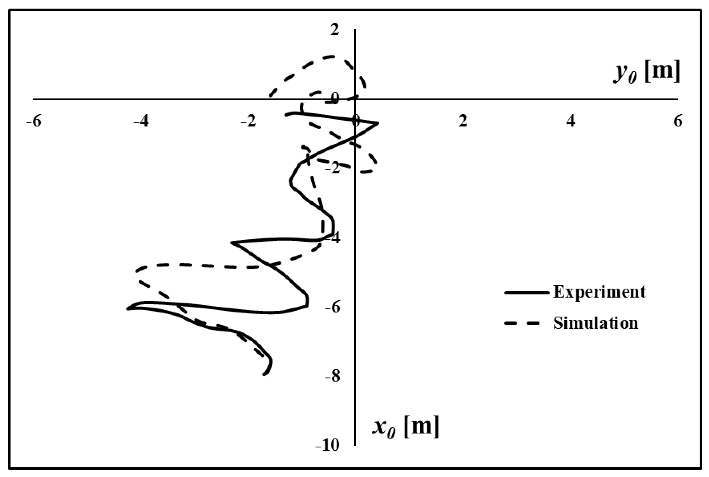
4.2. Actual Sea Area

Similarly, we conducted validation tests in the actual sea area at Nanao City, Ishikawa Prefecture, Japan, in August 2021. As shown in Figure 20, ten reference points (P1~P10) were set for testing. The Quadmaran vessel ran in the straight navigation mode (Figure 2d) between two reference points, and transitioned into the DP mode when the target reference point was within 10 m. Further, once the reference point was within 2 m, a one-minute timer was turned on. Within this one minute, the vessel arrived at the reference point in DP model. After the timer ended, the vessel switched back in to straight navigation mode and proceeded to the next point.

At P1~P5, all propellers were operated. As in the calm water area tests, only two propellers that rotate forward were operated at P6~P10. The overall recorded route of the Quadmaran vessel is depicted in Figure 21.

The wind speed measured on the test day varied between 2 and 4 m/s. From Figure 21, we can see that the Quadmaran vessel sailed well under such wind conditions and followed the established route. It was also confirmed that the vessel could complete tasks such as Dynamic Positioning at each reference point.

Here, we utilized the computational model to predict the motion during DP for P6, P8, and P10 reference points. Figure 22, Figure 23 and Figure 24 compare the experiment and simulation results. Since the wind speed fluctuated from moment to moment, the average measurement value during DP was used for the calculation. From the comparisons, we found that the developed computational model could predict the motion during DP with an accuracy of roughly 2 m, even when during wind conditions of up to 4 m/s. It showed the effectiveness of the wind calculation model, and is reliable to use for predicting the motion during DP of the vessel.

In addition, from the validation results in the calm water area and actual sea area, we found that slow motions can be captured well through oblique towing tests and static turning tests based on the quasi-static motion assumption. Through the computational model, we now have a deeper understanding of the motion characteristics of the Quadmaran vessel while in DP. The method can be used as a basis for multi-hull navigation vessels to predict and improve the DP performance.

5. Conclusions

This study developed a predictive model for the dynamic positioning motion simulation of a vessel with four hulls. The hydrodynamic coefficients were obtained through a series of oblique tank tests and static turning tests using a 1/3 scale model, and the propeller’s performance curve was derived from the Propeller Open Test. A simple wind force model was established based on the wind load test results of a single hull and the superstructure. Validation navigation tests were carried out in calm water, as well as windy sea areas. The calculation margin of error was kept within 2 m by the model created under the quasi-static assumption. Such results are considered satisfactory for systems with multiple error sources, including position recorders, compasses, and mechanical component delays. Specific findings obtained from this study are summarized below.

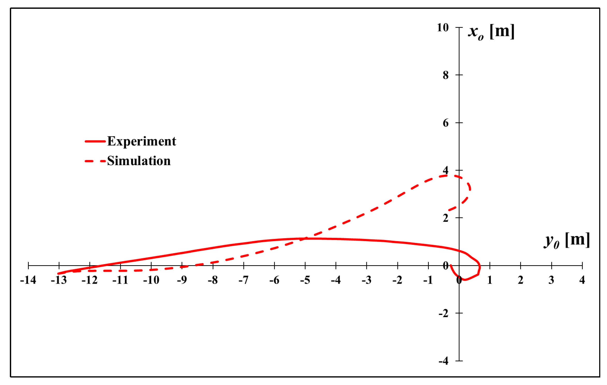
• The Quadmaran vessel can be dynamically positioned and kept within 2 m of the target point, under wind speeds not exceeding 5 m/s, as observed in actual sea tests.
• The drift angle of the vessel had a significant effect on the water loads generated from the parallel motion. The parallel motion with a drift angle in the range of 20–45 degrees was likely to rapidly fluctuate the fluid force due to the unique hull shape. The moment generated from the static yawing motion was almost proportional to the square of the yaw rate. The thrust coefficient (K_T) decreased as the advance ratio (J) increased when rotating forward, and was almost constant when reversing.
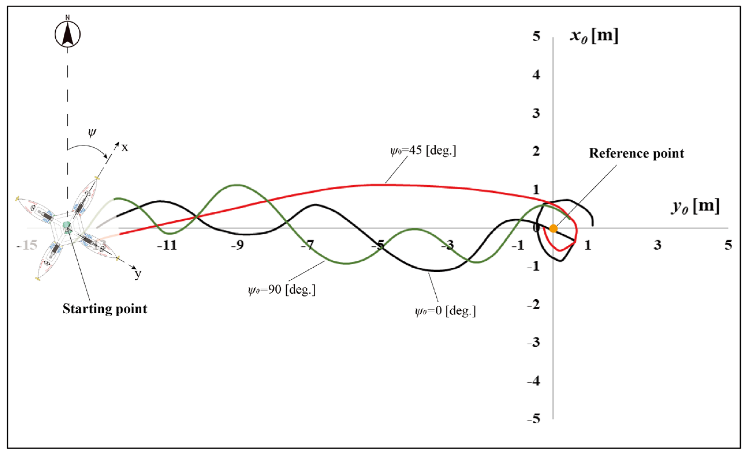
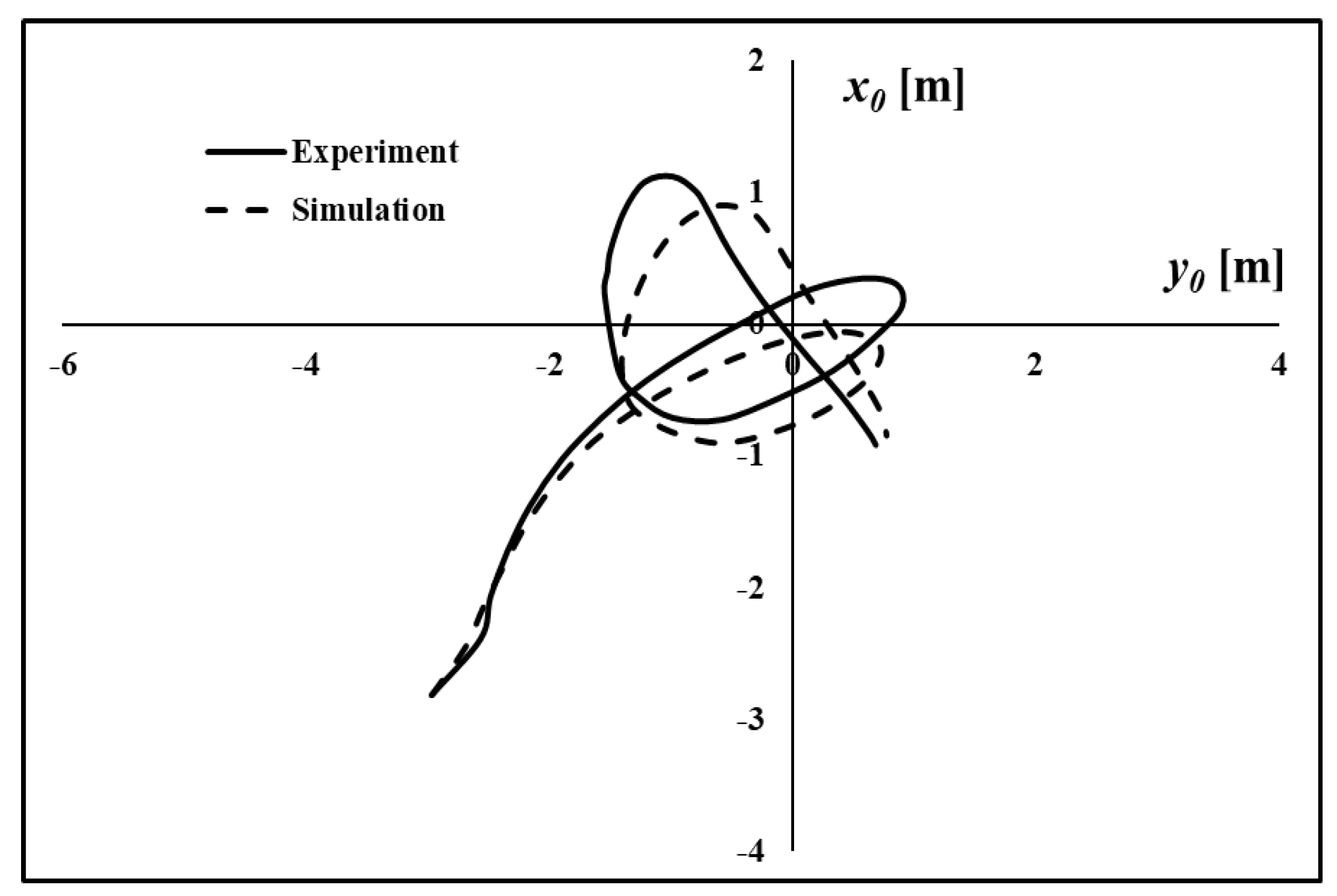
• The wind loads calculation model, which was established based on the database of wind load tests on a single hull and the superstructure, was found to be reliable in predicting the motion during DP of the vessel. The initial heading angle had some significance to the path of trajectory of the Quadmaran vessel in DP mode, but did not affect the prediction model if the loads were accurately assessed.
• The fluid force coefficient, assuming a quasi-static hull motion, was sufficiently accurate to predict the motion in DP mode. Therefore, the developed computational model can be useful to understand the motion characteristics of similar multi-hull vessels.

References

1. Japan Fisheries Agency: White Paper on Fisheries. Available online: https://www.jfa.maff.go.jp/j/kikaku/wpaper/h30_h/trend/1/t1_3_2_1.html (accessed on 29 June 2022).
2. Fauzi, R.; Jaya, I.; Iqbal, M. Unmanned Surface Vehicle (USV) Performance Test in Bintan Island Waters. IOP Conf. Ser. Earth Environ. Sci. 2021, 944, 012013. [Google Scholar] [CrossRef]
3. Lubczonek, J.; Kazimierski, W.; Zaniewicz, G.; Lacka, M. Methodology for Combining Data Acquired by Unmanned Surface and Aerial Vehicles to Create Digital Bathymetric Models in Shallow and Ultra-Shallow Waters. Remote Sens. 2021, 14, 105. [Google Scholar] [CrossRef]
4. Liang, J.; Zhang, J.; Ma, Y.; Zhang, C.-Y. Derivation of Bathymetry from High-Resolution Optical Satellite Imagery and USV Sounding Data. Mar. Geod. 2017, 40, 466–479. [Google Scholar] [CrossRef]
5. Stateczny, A.; Specht, C.; Specht, M.; Brčić, D.; Jugović, A.; Widźgowski, S.; Wiśniewska, M.; Lewicka, O. Study on the Positioning Accuracy of GNSS/INS Systems Supported by DGPS and RTK Receivers for Hydrographic Surveys. Energies 2021, 14, 7413. [Google Scholar] [CrossRef]
6. Komizo, M.; Mukai, K.; Hara, N.; Nihei, Y.; Konishi, K. Sea Testing of Automatic Motion Control System for a Quad-Maran Unmanned Vessel. In Proceedings of the 2019 International Automatic Control Conference (CACS), Keelung, Taiwan, 13–16 November 2019; pp. 1–6. [Google Scholar]
7. Kamio, K.; Tsurumi, Y.; Sakamoto, H.; Mishina, H.; Masuda, N.; Nakada, S.; Nihei, Y. Development of Water Quality Observation System in Shallow Water Using a Quadmaran Automated Vessel. J. Jpn. Soc. Civ. Eng. Ser. B1 Hydraul. Eng. 2021, 77, I_883–I_888. [Google Scholar] [CrossRef]
8. Nakada, S.; Mishina, H.; Kamio, K.; Masuda, N.; Nihei, Y. Monitoring for low-salinity water for aquafarm in hichirippu lagoon using quadmaran automated vessel. J. Jpn. Soc. Civ. Eng. Ser. B2 Coast. Eng. 2021, 77, I_871–I_876. [Google Scholar] [CrossRef]
9. Nihei, Y.; Kitamura, S.; Miyamoto, K.; Sotojo, M.; Ishii, Y.; Chikamoto, M.; Shinoi, T.; Masuda, N. Ships. 2017. Available online: https://patents.google.com/patent/JP6332824B1/en?oq=Patent+No.+6332824 (accessed on 30 June 2022).
10. Komizo, M.; Zhang, C.; Hara, N.; Nihei, Y.; Konishi, K. At-Sea Test of Dynamic Positioning System for a Quad-Maran Unmanned Vessel. In Proceedings of the 18th International Conference on Control, Automation and Systems, PyeongChang, Korea, 17–20 October 2018; pp. 682–684. [Google Scholar]
11. Sørensen, A.J. A Survey of Dynamic Positioning Control Systems. Annu. Rev. Control 2011, 35, 123–136. [Google Scholar] [CrossRef]
12. Sotnikova, M.V.; Veremey, E.I. Dynamic Positioning Based on Nonlinear MPC. IFAC Proc. Vol. 2013, 46, 37–42. [Google Scholar] [CrossRef]
13. Wang, L.; Yang, J.; Xu, S. Dynamic Positioning Capability Analysis for Marine Vessels Based on A DPCap Polar Plot Program. China Ocean. Eng. 2018, 32, 90–98. [Google Scholar] [CrossRef]
14. Arditti, F.; Cozijn, H.; Van Daalen, E.F.G.; Tannuri, E.A. Dynamic Positioning Simulations of a Thrust Allocation Algorithm Considering Hydrodynamic Interactions. IFAC PapersOnLine 2018, 51, 122–127. [Google Scholar] [CrossRef]
15. Ikeda, Y.; Katayama, T.; Okumura, H. Characteristics of Hydrodynamic Derivatives In Maneuvering Equations For Super High-Speed Planing Hulls. In Proceedings of the Tenth International Offshore and Polar Engineering Conference, Seattle, WA, USA, 28 May–2 June 2000. [Google Scholar]
16. Sunarsih, S.; Priyanto, A.; Zamani, M.; Izzuddin, N. A Chebyshev Polynomial on Torque and Thrust Coefficients of Mathematical Propeller Properties for a LNG Manoeuvring Simulation. J. Ocean. Mech. Aerosp. Sci. Eng. 2014, 11, 11–20. [Google Scholar]
17. Ji, M.; Srinivasamurthy, S.; Nihei, Y. Basic Research on the Influence of Descent Flow From Small Unmanned Aerial Vehicle (Quadcopter) on a Small Floating Body. In Proceedings of the ASME 2020 39th International Conference on Ocean, Offshore and Arctic Engineering, Virtual, 3–7 August 2020; Volume 6A, p. V06AT06A034. [Google Scholar]
18. Ogawa, A.; Koyama, T.; Kijima, K. MMG report-I, on the mathematical model of ship manoeuvring. Bull. Soc. Nav. Arch. Jpn. 1977, 575, 192–198. [Google Scholar]
19. Kazuo, S.; Noriyuki, S.; Takahumi, K. Hull Resistance and Propulsion; Marine Engineering; Seizando-Shoten Publishing Co., Ltd.: Shinjuku City, Japan, 2012. [Google Scholar]
20. Hewins, E.F.; Chase, H.J.; Ruiz, A.L. The Backing Power of Geared Turbine Driven Vessels. Annu. Meet. Soc. Nav. Archit. Mar. Eng. 1950, 58, 276–283. [Google Scholar]
21. Nihei, Y.; Tsurumi, Y.; Masuda, N.; Harada, K.; Okuno, J.; Hara, N.; Nakada, S. Automatic And Frequent Measurement Of Water Quality at Multi-Points Using Quadmaran. J. JSCE Ser. B1 2020, 76, I_1039–I_1044. [Google Scholar] [CrossRef]
22. Tsurumi, Y. A Study on Speed Estimation of Quadmaran under Wind Pressure; Osaka Prefecture University: Osaka, Japan, 2019. [Google Scholar]
23. High-Precision Positioning Service Ichimill. Available online: https://www.softbank.jp/biz/services/analytics/ichimill/ (accessed on 29 June 2022).
Figure 1. The Quadmaran vessel sailing on the sea.
Applsci 12 08759 g001
Figure 2. Quadmaran vessel—Modes of operations.
Applsci 12 08759 g002
Figure 3. Principal dimensions of the Quadmaran vessel.
Applsci 12 08759 g003
Figure 4. 1/3 scale model of a Quadmaran vessel.
Applsci 12 08759 g004
Figure 5. Principal dimensions of the 1/3 scale model.
Applsci 12 08759 g005
Figure 6. The coordinate system.
Applsci 12 08759 g006
Figure 7. Oblique towing test.
Applsci 12 08759 g007
Figure 8. Variation of the fluid force with the drift angle: (a) x-axis; (b) y-axis.
Applsci 12 08759 g008
Figure 9. (a) Variation of the dimensionless fluid force along the x-axis with u′; (b) Variation of the dimensionless fluid force along the y-axis with v′.
Applsci 12 08759 g009
Figure 10. (a) Variation of the yaw moment along the z-axis with the drift angle; (b) Variation of the dimensionless yaw moment along the z-axis with v′.
Applsci 12 08759 g010
Figure 11. (a) Variation of the yaw moment due to static rotation motion along the z-axis with the yaw rate; (b) Yaw moment coefficient.
Applsci 12 08759 g011
Figure 12. (a) Propeller; (b) Propeller Open Test.
Applsci 12 08759 g012
Figure 13. KT of four quadrants.
Applsci 12 08759 g013
Figure 14. The coordinate system of wind load.
Applsci 12 08759 g014
Figure 15. Running test scene in calm water.
Applsci 12 08759 g015
Figure 16. The trajectory of the running tests in calm water.
Applsci 12 08759 g016
Figure 17. Comparison of experiment and simulation when the initial heading angle is 0 degrees.
Applsci 12 08759 g017
Figure 18. Comparison of experiment and simulation when the initial heading angle is 45 degrees.
Applsci 12 08759 g018
Figure 19. Comparison of experiment and simulation when the initial heading angle is 90 degrees.
Applsci 12 08759 g019
Figure 20. Validation tests in the actual sea area.
Applsci 12 08759 g020
Figure 21. The route of the navigation tests in the actual sea area.
Applsci 12 08759 g021
Figure 22. Comparison of experiment and simulation at P6.
Applsci 12 08759 g022
Figure 23. Comparison of experiment and simulation at P8.
Applsci 12 08759 g023
Figure 24. Comparison of experiment and simulation at P10.
Applsci 12 08759 g024