Electric Vehicle Transient Speed Control Based on Vector Control FM-PI Speed Controller for Induction Motor

Abstract

The speed control of induction machines for multiple-speed handling is critical. When the vector control method is applied to induction machines, it has a significant impact on speed utilization. This strategy of operating the machine at a fixed predefined speed mode presents better results for electric vehicles. An effective model for a speed control loop is proposed in this paper, using a fixed-mode proportional integral (FM-PI) controller based on an upper and lower limit torque limiter. The power supply is fed using a lithium-ion battery with an inverter-fed mechanism. Moreover, the proposed model is validated using simulations with user-defined speed modes (40, 60, and 80 km/h). These speed modes, with different torque commands, have been considered for advanced modeling. In this model, torque is developed via a closed-loop control operation to attain the required speed assigned by the user. The sensors are used to collect data, and a multiple regression algorithm analyzes the dataset to predict input parameters (voltage (V_ab), phase current (I), and torque (T)) required to achieve the desired speed mode. The efficiency of the proposed model is compared with induction motors bearing the same rating for the loaded and unloaded speed test. Effective machine parameter control is achieved by reaching the desired performance levels of 94.37% and 78.30% in a shorter time for the loaded and unloaded modes. A speed response comparison of the FOPID, KW-WOA-PID, SVR-PI, and FM-PI controller model simulation results indicates that the FM-PI speed controller guarantees better performance and displays an improvement in rising time and settling time, compared to other controllers. The implementation of different driving scenarios proves the model’s effectiveness for robust speed applications.

1. Introduction

The energy consumption of the transportation sector is responsible for one-quarter of the entire fuel demand around the globe, and this is expected to rise exponentially, with an accompanying harmful impact on the environment in the form of climate change. A study reveals that electric vehicles (EVs) would reduce 45% of the daily carbon emissions and are proven to be environmentally friendly. An increase in the number of EV charging stations has further improved their reliability [1]. Induction motor (IM) drives are employed in all types of steady-state and dynamic applications and play an important role in modeling an electric vehicle (EV). The continuous monitoring of various electrical and mechanical parameters of induction motors is required for the efficient performance of EVs. The IM architecture and control strategies need improved modeling, in situations where the major considerations are steady-state and dynamic response, as per system demand.

Different approaches have been considered in the past for effective speed control in IM drives, such as the closed-loop vector control approach. This is applicable for variable frequency drives in which a three-phase stator current is mapped as orthogonal components to present a vector for analysis. This controls the machine in the same way as a separately activated direct current (DC) motor and replicates all its advantages with the IM. Vector control can achieve the desired level of reference speed and is equipped with faster switching to address issues that have been faced in previous designs, e.g., torque variations [2].

The research aims are as follows:

• To operate an EV on fixed speed modes (40, 60, and 80 km/h) for diverse loaded and unloaded driving situations.
• To design an efficient Li-ion DC battery-powered indirect vector-controlled IM-based EV model containing an FM-PI controller operating at user-defined fixed speed levels, with its performance monitored at predefined speed modes, as mentioned earlier.
• To record data sets of input (voltage (V_ab), phase current (I), torque (T)), and output (speed (${\mathsf{\omega }}_{\mathrm{r}}$ )) parameters and analyze them using multiple regression algorithm to achieve the desired speed mode.
• EV mileage tends to improve with an EV operating in a fixed-speed mode. The FM-PI controller performance has been analyzed. The established model contributes a reliable approach to handling diverse driving situations.

The paper has been structured in the following order: Section 2 presents a literature review to provide a detailed structure of previous research and publications in this field. Section 3 provides the modeling approach for the proposed system while considering machine parameters and generating waveforms for a proper understanding of the various speed mode inputs. Section 4 offers a detailed analysis of the model’s performance compared to other controllers and control operations to achieve the desired speed. The conclusion and future prospects are presented in Section 5.

2. Materials and Methods

This section summarizes the various aspects associated with research on induction machines. The phasor diagram of indirect vector control is shown in Figure 1, while the synchronous reference frame mode of the induction machine can be expressed as in Equation (1):

$$\left[\begin{array}{c}{\mathrm{V}}_{\mathrm{qs}}^{\mathrm{e}}\\ {\mathrm{V}}_{\mathrm{ds}}^{\mathrm{e}}\\ {\mathrm{V}}_{\mathrm{qr}}^{\mathrm{e}}\\ {\mathrm{V}}_{\begin{array}{c}\mathrm{d}\mathrm{r}\\ \mathrm{V}\end{array}}^{\mathrm{e}}\end{array}\right]=\left[\begin{array}{c}{\mathrm{R}}_{\mathrm{s}}+{\mathrm{L}}_{\mathrm{s}}\mathrm{P} {\mathsf{\omega }}_{\mathrm{s}}{\mathrm{L}}_{\mathrm{s}} {\mathrm{L}}_{\mathrm{m}}\mathrm{P} {\mathsf{\omega }}_{\mathrm{s}}{\mathrm{L}}_{\mathrm{m}} \\ -{\mathsf{\omega }}_{\mathrm{s}}{\mathrm{L}}_{\mathrm{s}} {\mathrm{R}}_{\mathrm{s}}+{\mathrm{L}}_{\mathrm{s}}\mathrm{P}-{\mathsf{\omega }}_{\mathrm{s}}{\mathrm{L}}_{\mathrm{m}} {\mathrm{L}}_{\mathrm{m}}\mathrm{P} \\ {\mathrm{L}}_{\mathrm{m}}\mathrm{P} ({\mathsf{\omega }}_{\mathrm{s}}-{\mathsf{\omega }}_{\mathrm{r}}){\mathrm{L}}_{\mathrm{m}} {\mathrm{R}}_{\mathrm{r}}+{\mathrm{L}}_{\mathrm{r}}\mathrm{P}({\mathsf{\omega }}_{\mathrm{s}}-{\mathsf{\omega }}_{\mathrm{r}}){\mathrm{L}}_{\mathrm{r}}\\ -({\mathsf{\omega }}_{\mathrm{s}}-{\mathsf{\omega }}_{\mathrm{r}}){\mathrm{L}}_{\mathrm{m}} {\mathrm{L}}_{\mathrm{m}}\mathrm{P} -({\mathsf{\omega }}_{\mathrm{s}}-{\mathsf{\omega }}_{\mathrm{r}}){\mathrm{L}}_{\mathrm{r}} {\mathrm{R}}_{\mathrm{r}}+{\mathrm{L}}_{\mathrm{r}}\mathrm{P} \end{array}\right].\left[\begin{array}{c}{\mathrm{i}}_{\mathrm{qs}}^{\mathrm{e}}\\ {\mathrm{i}}_{\mathrm{ds}}^{\mathrm{e}}\\ {\mathrm{i}}_{\mathrm{qr}}^{\mathrm{e}}\\ {\mathrm{i}}_{\mathrm{dr}}^{\mathrm{e}}\end{array}\right] .$$

(1)

Electromagnetic torque can be expressed as in Equation (2):

$${\mathrm{T}}_{\mathrm{e}}=\frac{3}{2}\frac{\mathrm{P}}{2}{\mathrm{L}}_{\mathrm{m}}\left({\mathrm{i}}_{\mathrm{qs}}^{\mathrm{e}}{\mathrm{i}}_{\mathrm{dr}}^{\mathrm{e}}-{\mathrm{i}}_{\mathrm{ds}}^{\mathrm{e}}{\mathrm{i}}_{\mathrm{qr}}^{\mathrm{e}}\right)$$

(2)

where:

${\mathsf{\omega }}_{\mathrm{s}}$: Synchronous speed

${\mathsf{\omega }}_{\mathrm{r}}$: Electrical speed (rotor speed)

P: Number poles of IM

${\mathrm{T}}_{\mathrm{e}}$: Electromagnetic torque

${\mathrm{L}}_{\mathrm{m}}$: Mutual inductance

${\mathrm{L}}_{\mathrm{s}}$: Stator leakage inductance

${\mathrm{L}}_{\mathrm{r}}$: Rotor leakage inductance

${\mathrm{R}}_{\mathrm{s}}$: Stator resistance

${\mathrm{R}}_{\mathrm{r}}$: Rotor resistance

${\mathrm{V}}_{\mathrm{qs}}^{\mathrm{e}}$: Stator voltage in the synchronous frame on the q-axis

${\mathrm{V}}_{\mathrm{ds}}^{\mathrm{e}}$: Stator voltage in the synchronous frame on the d-axis

${\mathrm{V}}_{\mathrm{qr}}^{\mathrm{e}}$: Rotor voltage in the synchronous frame on the q-axis

${\mathrm{V}}_{\mathrm{dr}}^{\mathrm{e}}$: Rotor voltage in the synchronous frame on the d-axis

${\mathrm{i}}_{\mathrm{qs}}^{\mathrm{e}}$: Stator current in the synchronous frame on the q-axis

${\mathrm{i}}_{\mathrm{ds}}^{\mathrm{e}}$: Stator current in the synchronous frame on the d-axis

${\mathrm{i}}_{\mathrm{qr}}^{\mathrm{e}}$: Rotor current in the synchronous frame on the q-axis

${\mathrm{i}}_{\mathrm{dr}}^{\mathrm{e}}$: Rotor current in the synchronous frame on the d-axis.

Making the appropriate choice of DC battery with effective performance is of considerable importance in many real-life applications. The Li-ion battery type is emerging as a source of enhanced energy, a better rating of power, and an improved charging/discharging cycle, with proficiency in the pulsated types of energy conversion systems. A preselected value for the charge/discharge cycle is essential to increase the lifetime of the Li-ion battery. Battery life-restrictive issues are defined as a drop in battery ability and are caused by a rise in the internal source resistance of DC batteries [3]. Generally, EVs are powered by a commercial battery management system (CBMS). The CBMS provides an alternative to traditional battery packs, which can cause thermal runaway loss. For this reason, individual batteries are often replaced by a commercial battery management system [4].

An inverter-fed mechanism is used to deliver a 3-phase supply to the IM. An IGBT inverter, operating at a higher switching frequency, performs better than the older models. A hysteresis-band PWM (pulse-width modulation) provides optimum performance over the inverter losses. The terminal voltages and respective currents or flux sense windings are included when determining the field angle for a direct vector control strategy [5]. PI-based controllers are more applicable as a way to regulate the torque and flux feedback toward reference values. The proportional controller decreases the rise time, whereas an integral controller eliminates steady-state error in order to attain the set parameters efficiently [6].

In a speed-sensorless vector-controlled induction drive, both torque and flux are controlled independently. Previous studies suggest that peak power is achieved by using incremental and conductance-based MPPT (maximum power point tracking) algorithms. [7]. The MRAS (model reference adaptive system) is another technique that can be used to provide a robust defense and effectively ensures good performance against variations in the parameters, noise removal, and error measurements The space vector modulation (SVM) technique imposes a tension vector through the vector modulation of space for a predictive selection of torque and flux [8]. The implementation of realistic multivariable analysis is preferred with decoupling-decentralized controllers. This technique is suitable for an analysis of the complex parameters in industrial control systems [9].

In terms of the hysteresis boundary, when the current regulator exceeds its limit, the terminal voltage of the inverter changes toward the upper limit or lower limit until a set voltage level is reached. The current error can be calculated by taking the current change rate [10,11]. The estimated value of inductance governs the simulation of an IM. Various factors can influence the calculated inductance value, e.g., the winding distribution rotor, stator slots, magnetic material saturation level, and asymmetric behavior due to various machine faults. The visualization of a 3-dimensional model of the induction motor is generally performed in Simulink [12,13]. A swing equation is applied to describe the relative motion in the case of rotor acceleration or deacceleration to accomplish the selected speed mode values. A transient stability calculation is employed for the behavioral assessment of a synchronous machine rotor during the transition period [14].

Unbalanced supply voltage impacts induction motor efficiency and is usually calculated with an estimation algorithm. The genetic algorithm uses a pre-tested dataset for motors, and the IEEE form F-2/F-1 method calculations are used for estimation-based analysis [14,15]. A particle swarm optimization algorithm is used for accurate estimation of the electrical parameters of IM. These results are helpful in the estimation of motor efficiency [16]. The efficiency of IM, either loaded or unloaded, is estimated via various experimental setups [17,18,19,20]. A study has presented a no-load test determining the efficiency of the IM by testing 129 motors, ranging from 1–500 hp, in a laboratory as per standard IEEE 112 TM procedures [21,22].

In some of the previous studies, the researchers have used different techniques for the desired operation and maintenance of IM, e.g., (a) a variable-gain PID controller implemented for the IM through vector control, which displayed improved sustainability in terms of EV acceleration [23]. (b) The IM power factor is measured using a support vector regression algorithm for loaded, unloaded, and overloaded scenarios [24]. (c) The IM operating conditions are monitored using a multiple regression algorithm with optimization of the genetic algorithm. This predicts short circuits and normal operations with considerable accuracy [25].

The major concern in speed control operation in the case of indirect vector control of IM is the smooth output speed curve. In a recent study, indirect vector control, comprising a fuzzy fractional-order PID (FOPID) controller, contributes to a better tracking reference speed. The FOPID controller implements an ant-colony optimization algorithm for the robust speed-tracking of EV. Apart from the design of the fuzzy control parameters, better tuning of PI control parameters can significantly improve system performance in diverse situations [17]. The researchers believe that an EV operating at a predefined speed contributes to the mileage and efficiency of that EV [26].

3. The Proposed PI-Tuned Speed Controller

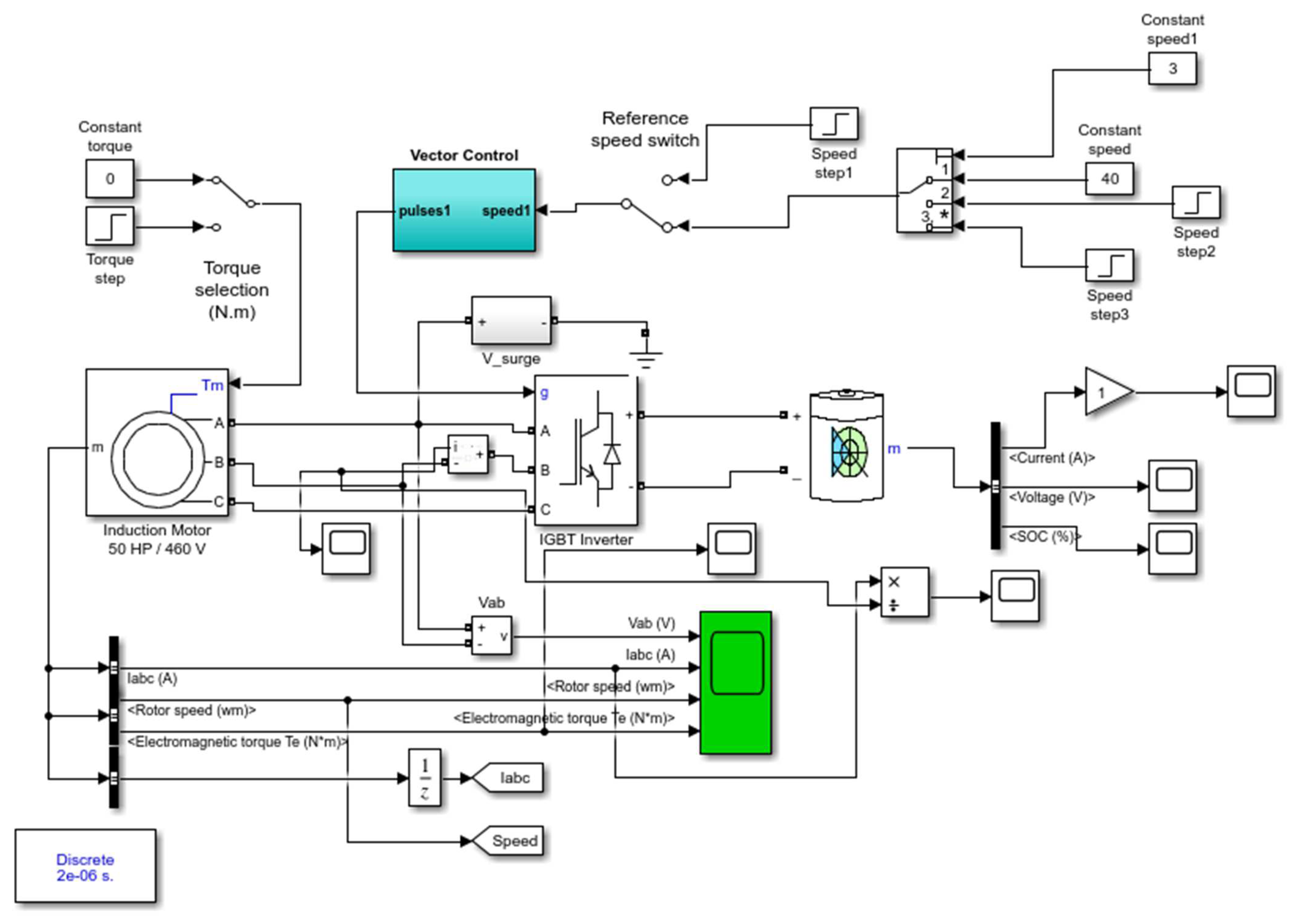
The model under consideration is based on a Li-ion DC battery with the scope to check the performance of the supply voltage. DC voltage is converted into a three-phase AC supply by using an IGBT inverter. The IGBT inverter gate pulses are fed by the speed control loop of the vector control. The output of the IGBT inverter is applied to IM to the drive for the applied speed commands. The output of the IM speed control model is measured to analyze the performance of the EV.

The proposed multimodal EV is applicable for the desired speed modes, based on the current situation and road signals, to ensure a smooth and efficient drive. The user-defined speed mode works as a reference for the speed controller, and after the control action of the PI controller, the gate pulses for inverter operation are generated. The battery is initially charged at 770 V, while temperature and aging effects (due to the battery’s lifecycle) are not considered.

In terms of indirect vector control, two current components are used to change the value of flux and torque, as per the speed command. Figure 2 presents a block diagram of P-I controller-based indirect vector control.

The required angle ${\mathsf{\theta }}_{\mathrm{e}}$ is calculated using the vector control currents ${\mathrm{i}}_{\mathrm{qs}}^{*}$ and ${\mathrm{i}}_{\mathrm{ds}}^{*}$, further transformed from a synchronously rotating frame to a stationary vector frame with the help of angle ${\mathsf{\theta }}_{\mathrm{e}}$, and produced from the flux value. Stationary vector frame current signals are converted into phase current signals to compare the measured phase currents and generate gating pulses for the IGBT inverter. The gate pulses are used to get a 3-phase supply from an IGBT-based inverter, fed by a Li-ion DC battery. The inverter-based supply is directly fed to an IM for suitable output. The input and output parameters are displayed to analyze model performance for the various speed modes (40, 60, and 80 km/h).

The model operation starts with a user-defined reference speed to implement an automatic car model. Reference speed and torque are applied as separate inputs to IM, using a manually operated switch block. The respective reference speeds of 40, 60, and 80 km/h, with torque at (0 and 100 N m), are applied on IM. These three-speed modes are defined to summarize the model’s behavior for user-defined drive patterns. IM speed ω is compared with the reference speed provided by the user ${\mathsf{\omega }}^{*}$ for the tuning of FM-PI controller gains. Feedback on measured speed is continuously monitored for closed-loop control action. A discrete (P-I) controller processes (as a speed difference) an error signal without automatic tuning, followed by a saturator to maintain the torque command ${\mathrm{T}}_{\mathrm{e}}^{*}$ within an upper and lower limit, as shown in Figure 3. The role of the speed controller is to monitor the speed at a steady state as well as for transients. The gain of the P-I controllers is tuned to achieve an optimum damping ratio (less than unity), kept at ${\mathrm{K}}_{\mathrm{p}}$ = 15 and ${\mathrm{K}}_{\mathrm{i}}$ = 30 for a maximum upper torque limit of 300 N m.

The stator direct-axis current ${\mathrm{i}}_{\mathrm{ds}}$ forming the rotor flux and torque is directly linked to the quadrature-axis current, ${\mathrm{i}}_{\mathrm{qs}}$, whereas the reference quadrature axis current ${\mathrm{i}}_{\mathrm{qs}}^{*}$ is computed from the reference torque ${\mathrm{T}}_{\mathrm{e}}^{*}$ as an input variable in Equation (3), while ${\left|\mathsf{\Psi }\mathrm{r}\right|}_{\mathrm{est}}$ and ${\mathrm{T}}_{\mathrm{r}}$ are calculated from Equations (4) and (5), respectively.

$${\mathrm{i}}_{\mathrm{qs}}^{*}=(\frac{2}{3}).(\frac{2}{\mathrm{P}}).(\frac{{\mathrm{L}}_{\mathrm{r}}}{{\mathrm{L}}_{\mathrm{m}}}).(\frac{{\mathrm{T}}_{\mathrm{e}}^{*}}{{\left|\mathsf{\Psi }\mathrm{r}\right|}_{\mathrm{est}}})$$

(3)

$${\left|\mathsf{\Psi }\mathrm{r}\right|}_{\mathrm{est}}=\frac{{\mathrm{L}}_{\mathrm{m}}.{\mathrm{i}}_{\mathrm{ds}}}{1+{\mathrm{T}}_{\mathrm{r}}.\mathrm{s}}$$

(4)

$${\mathrm{T}}_{\mathrm{r}}=\frac{{\mathrm{L}}_{\mathrm{r}}}{{\mathrm{R}}_{\mathrm{r}}}$$

(5)

Here, P is the number of poles, ${\left|\mathsf{\Psi }\mathrm{r}\right|}_{\mathrm{est}}$ is the estimated rotor flux, ${\mathrm{L}}_{\mathrm{r}} \mathrm{and} {\mathrm{L}}_{\mathrm{m}}$ are rotor inductance and motor inductance, respectively, while ${\mathrm{R}}_{\mathrm{r}}$ is the rotor resistance and ${\mathrm{T}}_{\mathrm{r}}$ is the rotor time constant. Here, ${\mathrm{L}}_{\mathrm{r}}$ is calculated via Equation (6). Rotor frequency ${\mathsf{\omega }}_{\mathrm{r}}$ is measured using Equation (7). The direct axis reference current ${\mathrm{i}}_{\mathrm{ds}}^{*}$ is found by taking the rotor flux reference input ${\left|{\mathsf{\Psi }}_{\mathrm{r}}\right|}^{*}$ in Equation (8).

$${\mathrm{L}}_{\mathrm{r}}={\mathrm{L}}_{\mathrm{Ir}}+{\mathrm{L}}_{\mathrm{m}}$$

(6)

$${\mathsf{\omega }}_{\mathrm{r}}=\frac{{\mathrm{L}}_{\mathrm{m}} .{\mathrm{I}}_{\mathrm{q}}}{{\mathrm{T}}_{\mathrm{r}} .{\left|\mathsf{\Psi }\mathrm{r}\right|}^{*}}$$

(7)

$${\mathrm{i}}_{\mathrm{ds}}^{*}=\frac{{\left|\mathsf{\Psi }\mathrm{r}\right|}^{*}}{{\mathrm{L}}_{\mathrm{m}}}$$

(8)

Here, ${\mathrm{L}}_{\mathrm{Ir}}$ is rotor leakage inductance, the rotor flux angle ${\mathsf{\theta }}_{\mathrm{e}}$ is utilized for the coordinate’s transformation from dq to ABC and the coordinate’s conversion from an ABC to a dq form, respectively. The above-mentioned angle is calculated from the integration taken for the sum of the rotor mechanical speed ${\mathsf{\omega }}_{\mathrm{m}},$ measured by the speed sensor, and rotor frequency ${\mathsf{\omega }}_{\mathrm{r}}$ in Equation (9), while rotor frequency is computed in Equation (3). For the ABC to dq transformation, the values of the measured 3-phase current ${\mathrm{I}}_{\mathrm{abc}}$ and rotor flux positions ${\mathsf{\theta }}_{\mathrm{e}}$ are used to generate dq currents for flux and theta generation, respectively.

$${\mathsf{\theta }}_{\mathrm{e}}=\int ({\mathsf{\omega }}_{\mathrm{r}}+{\mathsf{\omega }}_{\mathrm{m}})$$

(9)

DQ to ABC current conversion is calculated with Equations (10)–(12):

$${\mathrm{I}}_{\mathrm{a}}={\mathrm{I}}_{\mathrm{d}}\cos \mathsf{\theta }-{\mathrm{I}}_{\mathrm{q}}\cos \mathsf{\theta }$$

(10)

$${\mathrm{I}}_{\mathrm{b}}={\mathrm{I}}_{\mathrm{d}}\cos \left(\mathsf{\theta }-\frac{2}{3}\mathsf{\pi }\right)-{\mathrm{I}}_{\mathrm{q}}\sin \left(\mathsf{\theta }-\frac{2}{3}\mathsf{\pi }\right)$$

(11)

$${\mathrm{I}}_{\mathrm{c}}={\mathrm{I}}_{\mathrm{d}}\cos \left(\mathsf{\theta }+\frac{2}{3}\mathsf{\pi }\right)-{\mathrm{I}}_{\mathrm{q}}\sin \left(\mathsf{\theta }+\frac{2}{3}\mathsf{\pi }\right).$$

(12)

ABC to DQ current conversion is calculated with Equations (13) and (14):

$${\mathrm{I}}_{\mathrm{d}}=\frac{2}{3}\left({\mathrm{I}}_{\mathrm{a}}\cos \mathsf{\theta }+{\mathrm{I}}_{\mathrm{b}}\cos \left(\mathsf{\theta }-\frac{2}{3}\mathsf{\pi }\right)+{\mathrm{I}}_{\mathrm{c}}\cos \left(\mathsf{\theta }+\frac{2}{3}\mathsf{\pi }\right)\right)$$

(13)

$${\mathrm{I}}_{\mathrm{q}}=-\frac{2}{3}\left({\mathrm{I}}_{\mathrm{a}}\sin \mathsf{\theta }+{\mathrm{I}}_{\mathrm{b}}\sin \left(\mathsf{\theta }-\frac{2}{3}\mathsf{\pi }\right)+{\mathrm{I}}_{\mathrm{c}}\sin \left(\mathsf{\theta }+\frac{2}{3}\mathsf{\pi }\right)\right).$$

(14)

The ${\mathrm{i}}_{\mathrm{qs}}^{*}$ and ${\mathrm{i}}_{\mathrm{ds}}^{*}$ are the reference quadrature and reference direct currents, respectively. Both currents are converted into the 3-phase current references ${\mathrm{I}}_{\mathrm{abc}}^{*}$ through ${\mathsf{\theta }}_{\mathrm{e}}$ for calculations related to the current regulators. The role of the current regulator is to generate gate pulses for the IGBT inverter. The three-phase hysteresis current regulator is taking the measured ${\mathrm{I}}_{\mathrm{abc}}$ and reference ${\mathrm{I}}_{\mathrm{abc}}^{*}$ values to generate gate signals for the smooth operation of the IGBT inverter. The IM is implemented as an asynchronous machine Simulink block. The IM is supplied by a current-controlled PWM (IGBT)inverter, working as a three-phase AC source. 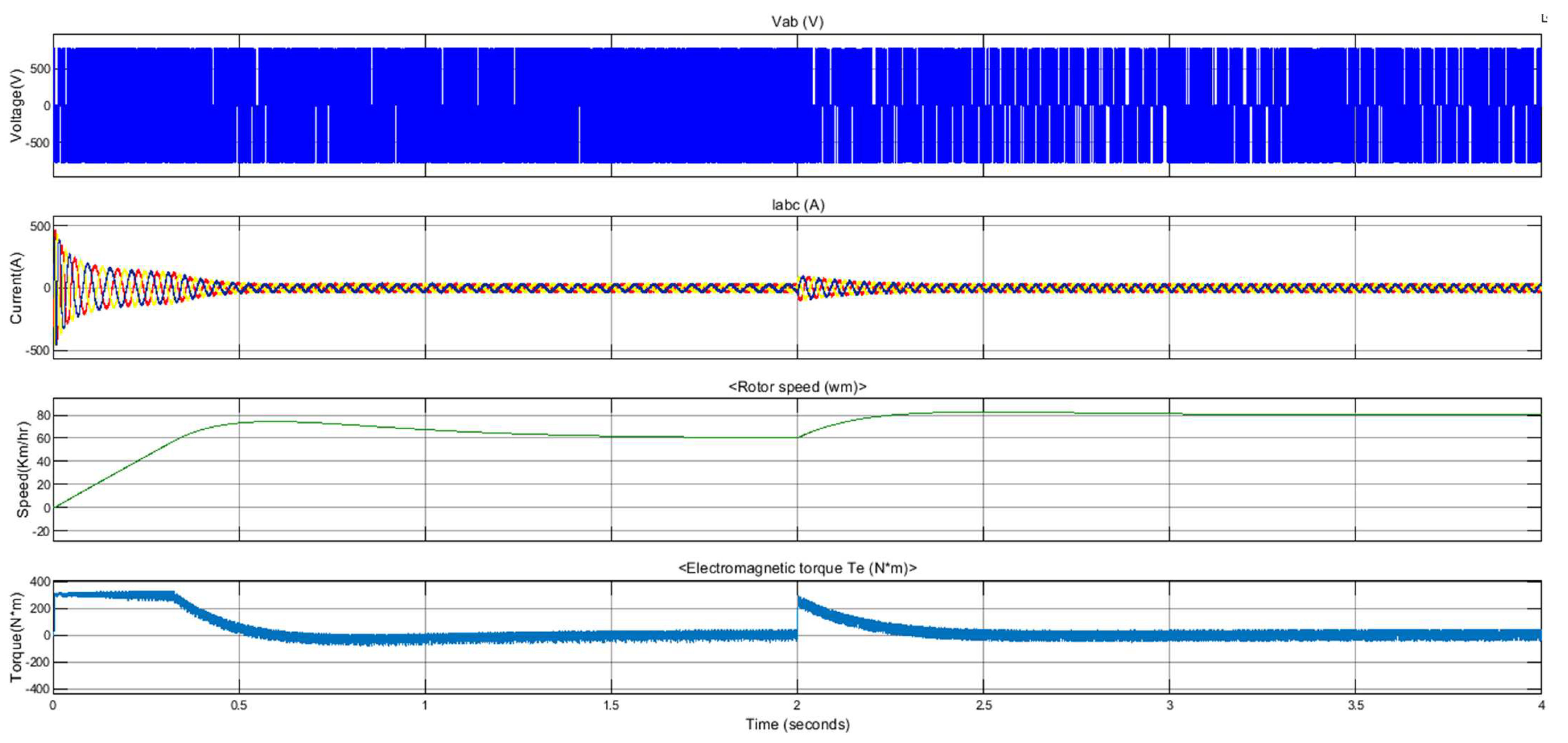The model developed in Simulink is presented in Figure 4. The output waveforms are generated for (a) voltage between two phases, (b) current (3-phase), (c) rotor speed, and (d) electromagnetic torque to analyze behavior at different time periods. The IM employed is set at 50 HP, 460 V, four-pole, and 60 Hz, with the parameters given in

Table 1. Induction machine electrical parameters.

Sr. No	Parameter Name	Impedance Parameters	Value
1	Stator winding resistance	Rs	87 mΩ
2	Stator leakage inductance	LIs	0.8 mH
3	Excitation inductance	Lm	34.7 mH
4	Rotor resistance	Rr	227 mΩ
5	Rotor leakage inductance	LIr	0.8 mH

.

The actions of the rotor and stator are synchronized by the swing equation. The purpose is to calculate the conversion efficiency from electrical power to mechanical power. The swing equation in terms of torque is calculated using Equation (15). Here, ${\mathrm{T}}_{\mathrm{m}}$, ${\mathrm{T}}_{\mathrm{g}},$ and ${\mathrm{T}}_{\mathrm{D}}$ are the mechanical, electrical, and damping torques, respectively.

$$\frac{{\mathrm{Jd}}^2{\mathsf{\delta }}_{\mathrm{m}}}{{\mathrm{dt}}^2}={\mathrm{T}}_{\mathrm{net}}=({\mathrm{T}}_{\mathrm{m}}-{\mathrm{T}}_{\mathrm{g}}-{\mathrm{T}}_{\mathrm{D}})$$

(15)

Here, Equation (14) can be re-written in terms of power by multiplying both sides with instantaneous mechanical speed input ${\mathsf{\omega }}_{\mathrm{m}},$ as in Equation (16):

$$\frac{{\mathrm{J}\mathsf{\omega }}_{\mathrm{m}}.{\mathrm{d}}^2{\mathsf{\delta }}_{\mathrm{m}}}{{\mathrm{dt}}^2} ={\mathrm{T}}_{\mathrm{net}} =({\mathrm{T}}_{\mathrm{m}}-{\mathrm{T}}_{\mathrm{g}}-{\mathrm{T}}_{\mathrm{D}}).{\mathsf{\omega }}_{\mathrm{m}}.$$

(16)

Different strategies have been used to achieve the relevant results [10,18]. The hysteresis-based current controller (CC) operates by relating a current error variation between the calculated and required 3-phase currents, versus a constant hysteresis band. An inner hysteresis band is employed to sense the changing moments via digital logic for use in Equation (17).

M, in Equation (18), is the angular momentum of the rotor at a synchronous speed. Here, ${\mathrm{P}}_{\mathrm{m}}$, ${\mathrm{P}}_{\mathrm{g}},$ and ${\mathrm{P}}_{\mathrm{D}}$ are the mechanical, electrical, and damping power in MW (megawatts), respectively. In various swing equations, the parameter H is the merged inertia constant of the prime mover–generator–exciter system, expressed in seconds. It is generally accepted to have a time range of (1–10) seconds for all types of machines under test; the calculated value is based upon the three-phase MVA ratings of the IM under examination, as given in Equation (19).

$$\frac{\mathrm{M}.{\mathrm{d}}^2{\mathsf{\delta }}_{\mathrm{m}}}{{\mathrm{dt}}^2}={\mathrm{P}}_{\mathrm{net}} =({\mathrm{P}}_{\mathrm{m}} -{\mathrm{P}}_{\mathrm{g}}-{\mathrm{P}}_{\mathrm{D}})$$

(17)

$$\mathrm{M}=\mathrm{J}.{\mathsf{\omega }}_{\mathrm{m}}$$

(18)

$$\mathrm{H}=\frac{{\mathrm{J}\mathsf{\omega }}_{\mathrm{s}}^2}{2.{\mathrm{S}}_{\mathrm{rated}}}$$

(19)

After substituting M (Equation (18)) into Equation (17), Equation (20) is obtained:

$$2\mathrm{H}\text{·}\left(\frac{{\mathrm{S}}_{\mathrm{rated}}}{{\mathsf{\omega }}_{\mathrm{s}}^2}\right){\mathsf{\omega }}_{\mathrm{m}}.\left(\frac{{\mathrm{d}}^2{\mathsf{\delta }}_{\mathrm{m}}}{{\mathrm{dt}}^2}\right)={\mathrm{P}}_{\mathrm{net}}=({\mathrm{P}}_{\mathrm{m}}-{\mathrm{P}}_{\mathrm{g}}-{\mathrm{P}}_{\mathrm{D}}).$$

(20)

Finally, the present net power P_net is calculated in Equation (21):

$$\left(\frac{2\mathrm{H}}{2.{\mathsf{\omega }}_s}\right).\left(\frac{{\mathrm{d}}^2{\mathsf{\delta }}_{\mathrm{m}}}{{\mathrm{dt}}^2}\right)={\mathrm{P}}_{\mathrm{net}}=({\mathrm{P}}_{\mathrm{m}}-{\mathrm{P}}_{\mathrm{g}}-{\mathrm{P}}_{\mathrm{D}}).$$

(21)

The dataset for the proposed model is derived from Figure 5. The input parameter voltage (V_ab), phase current (I), torque (T), and output parameter speed (${\mathsf{\omega }}_{\mathrm{r}}$) are recorded for 1 million time samples. The dataset of both the input and output parameters is loaded into a multiple regression algorithm for predictive analysis. Then, the multiple linear regression algorithm predicts the speed from the input parameters of voltage (V_ab), phase current (I), and torque (T), respectively. The mathematical equations of the regression algorithm are presented as Equations (22) and (23):

$${\mathrm{y}}_{\mathrm{i}}={{\displaystyle \sum }}_{\mathrm{i}=1}^{\mathrm{n}}\mathrm{f}({\mathrm{x}}_{\mathrm{i}},\mathsf{\beta })+{\mathsf{\epsilon }}_{\mathrm{i}}$$

(22)

$${\mathrm{y}}_{\mathrm{i}}=\mathrm{f}\left({\mathrm{x}}_{\mathrm{i}},\mathsf{\beta }\right)$$

(23)

where ${\mathsf{\epsilon }}_{\mathrm{i}}$ is the difference between actual and estimated value, $\mathrm{f}\left({\mathrm{x}}_{\mathrm{i}},\mathsf{\beta }\right)$ is a polynomial equation, ${\mathrm{x}}_{\mathrm{i}}$ is the number of independent variables, and $\mathsf{\beta }$ is the coefficient of the polynomial equation. In the case of input voltage (V_ab), phase current (I), torque(T), and output speed (${\mathsf{\omega }}_{\mathrm{r}}$) Equation (24) is utilized:

$${\mathsf{\omega }}_{\mathrm{r}}={\mathsf{\beta }}_0+{\mathsf{\beta }}_1{\mathrm{V}}_{\mathrm{ab}}+{\mathsf{\beta }}_2\mathrm{I}+{\mathsf{\beta }}_3\mathrm{T}$$

(24)

where ${\mathsf{\beta }}_0$ is the intercept, ${\mathsf{\beta }}_1$ is the slope of (voltage (V_ab)), ${\mathsf{\beta }}_2$ is the slope of (phase current (I)), ${\mathsf{\beta }}_3$ is the slope of (torque (T)). Here, input voltage (V_ab), phase current (I), and torque (T) are the independent variables, while output (speed (${\mathsf{\omega }}_{\mathrm{r}}$)) is the dependent variable.

4. Discussion

As shown in Figure 5, the low-speed mode for EV is 40 km/h. It is evident from the waveform that the total time taken by the FM-PI controller is 1.4 s, with an overshoot of 12.5%. The IM begins operation from the rest position. Hence, the torque reaches its maximum limit of 300 Nm. Due to this huge torque value, a large current is required to change the state of the motor from rest to motion. As the control action proceeds towards the referenced speed, both torques, and the three phases, the current value drops exponentially. A zoom view of the phase-to-phase voltage, V_ab, is presented in Figure 6.

Figure 7 shows that the 60 km/h medium-speed mode is followed by 40 km/h in the lower speed mode. The control operation from the resting position to a lower speed takes 1.4 s, while it takes 1.1 s from low speed to medium speed. Hence, the total time taken by the FM-PI controller is 2.5 s, while the overshoot for the second speed transition is observed as 5%. The simulated model follows two reference speed commands to reach the step speed through a closed-loop PI control operation. Initially, the current and torque reach the maximum value. While the motor achieves a set speed value, at this point the current value drops with the decay in rotor torque, dropping to the minimum value. It reaches a stable speed at 3.1 s, with the torque and current both approaching minimum values.

As presented in Figure 8, the high-speed mode at 80 km/h is followed by a medium-speed mode at 60 km/h. The protocol to reach a high speed in less time is to adopt the medium-speed mode from the rest position, followed by a high-speed transition. For a speed step of 60 km/h, initially, the FM-PI controller takes 1.7 s to reach medium speed, while from the second transition at 2 s, it takes 1.1 s from medium speed to high speed. Therefore, the total time taken by the FM-PI controller is 2.8 s, while the overshoot for the second transition is 4%.

The general speed mode operation consists of four speed transitions, as presented in Figure 9. The model was subjected to a start from the rest position toward the low, medium, high, and brake transitions, respectively. The first step was at 40 km/h, then at 2.0 s for 40 km/h to 60 km/h. The next step was applied at 4.0 s for 60 km/h to 80 km/h, then, at 6.0 s, a brake was applied to deaccelerate the IM toward the rest position. At 2.0 s, the reference speed command instantly reached a value of from 40 to 60 km/h. The torque with the current reached the maximum value to attain the required speed as early as possible, through vector control. The same behavior was observed at 4.0 s for the reference speed step from 60 to 80 km/h. When the machine finally achieved a speed of 80 km/h at 5.1 s, with torque and current both approaching minimum values over time, at 6.0 s, the torque took a negative maximum of 300 N.m., and the speed dropped toward the resting state. Finally, it reached the rest position at 7.7 s. The overshoot of the first, second, and third transitions remained the same, while the undershoot in the fourth transition is 22%.

The additional driving scenario built for a load torque of 100 Nm, applied for low (40 km/h), medium (60 km/h), and high-speed modes (80 km/h), is presented in Figure 10. The waveform suggests that the PI-based model response time remained the same for all speed transitions. Figure 11 presents the speed transition from resting to low (40 km/h), then low (40 km/h) to high (80 km/h), and finally, from high (80 km/h) to low-speed mode (40 km/h), respectively. The first transition response time remained the same, while the second was 1.6 s and the third was 1.4 s. The overshoot of the first transition was 5%, and the overshoot of the second transition was 15%, while the undershoot of the third transition was 5%.

The waveform in Figure 12 represents the IM operation for the low (40 km/h) and high (80 km/h) speed modes. In Figure 12a, as the measured speed rises, the torque value falls. Figure 12b summarizes the variation in torque and phase current with a measured tracking speed mode of 40 km/h. The analysis suggests that as the desired speed is achieved, both the torque and phase current reach the minimum value accordingly. 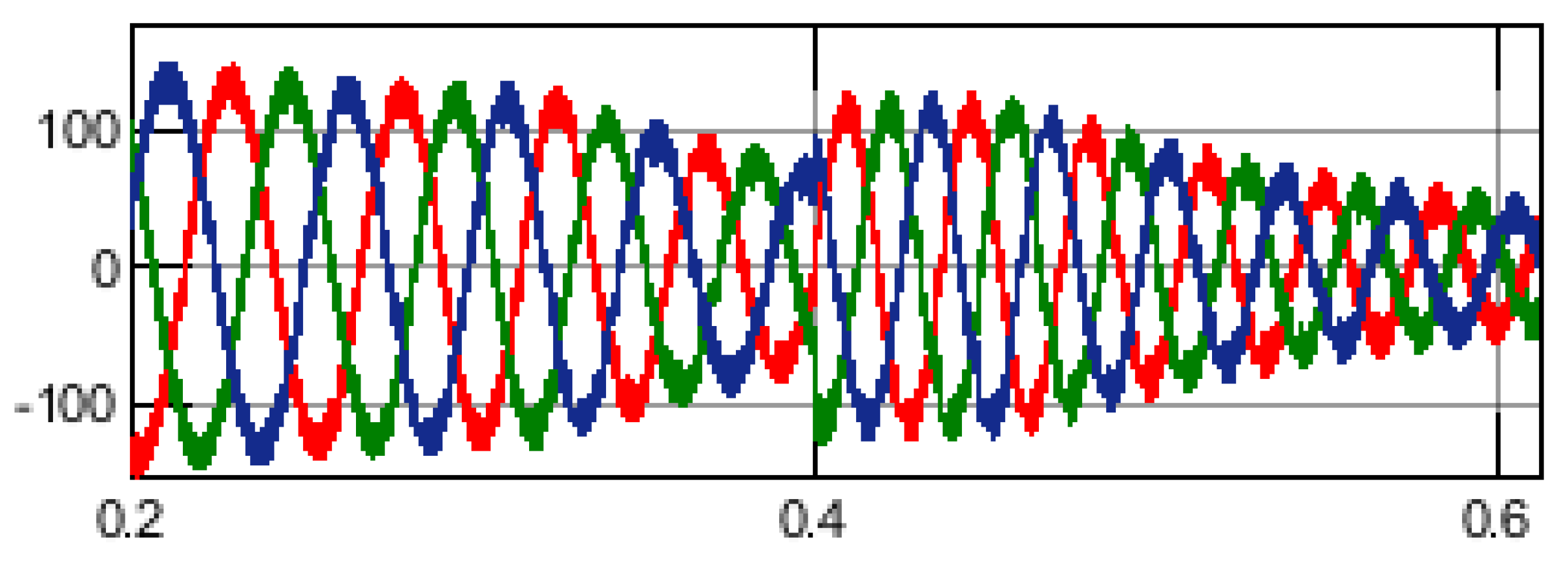Figure 12c portrays the variation of the three-phase current values at speed modes of 60 and 80 km/h. When the speed mode at 60 km/h is applied, the current reaches the maximum value; as the reference speed is achieved, the three-phase current value drops. When the next speed mode at 80 km/h is applied, the first current value rises; as the model tries to reach the reference speed of 80 km/h, the three-phase current value reaches its minimum value. Figure 13 presents a zoomed-in view of the variations in the three-phase voltage supply for the 60–80 km/h speed mode.

In the next step, the swing equation is implemented to calculate the accelerated power. The rotor angle, measured at a 2 s threshold for a 40 km/h speed command, is approximately 112°; this matches the results of the FFT analysis performed on the model. The calculated accelerated power is approximately 4.7 kW for both cases. This verifies the model validation for efficiency analysis.

In

Table 2. Efficiency results were calculated and measured for 15 different induction motors under test conditions, ranging from 1–500 hp.

Sr. No.	Power	Speed	Design	INS. CLASS	Measured Efficiency	Estimated Efficiency	Error [100%]
1	1	1745	B	F	0.844	0.853	0.69
2	3	1745	B	F	0.865	0.865	1.223
3	7.5	1750	B	F	0.877	0.881	0.744
4	10	1745	B	F	0.9	0.903	0.511
5	20	1770	B	F	0.923	0.924	0.596
6	30	1775	B	B	0.938	0.942	0.486
7	40	1180	B	F	0.932	0.928	1.509
8	50	1770	B	F	0.943	0.938	1.292
9	75	1777	B	F	0.92	0.926	0.042
10	100	1780	B	F	0.933	0.94	0.049
11	150	1780	B	F	0.942	0.935	1.177
12	200	1785	B	F	0.946	0.946	0.26
13	300	1790	B	F	0.952	0.952	0.361
14	400	1788	B	F	0.949	0.953	0.083
15	500	1185	B	F	0.947	0.947	0.398

, the error is calculated between measured and estimated efficiency (for the proposed algorithm, IEEE standard, and IEC standard) [23]. In the first stage, the speed of the IM of the experimental setup is converted to km/h using Equation (25). For 50 hp IM, 1770.0 rpm is converted into 266 km/h. Thus, after conversion, the required test speed of 60 km/h is calculated as 398 rpm.

K = d·r·(0.001885)

(25)

The mechanical output power is calculated by using the formula in Equation (26).

$${\mathrm{P}}_{\mathrm{m}}={\mathsf{\omega }}_{\mathrm{r}}·{\mathrm{T}}_{}$$

(26)

where “${\mathsf{\omega }}_{\mathrm{r}}$” denotes the rotor speed and T is the developed torque by the IM. The input power of IM is computed with the output power for efficiency calculations. Input power is calculated as 54,863 watts by taking the RMS current and phase voltage value. The mechanical form of the output power at 60 km/h speed is calculated as 42,970 watts. Therefore, the efficiency of the running model is 78.3%. The error percentage for the no-load condition is less than unity (0.5305%).

A drop in the efficiency of IM from 94.37% to 78.3% can be seen in Table 2 [24]. A decrease in IM efficiency from unloaded to loaded operation is observed, due to the loading effect applied to match the required speed mode. A drop in speed in the given proposed model indicates that the loaded motor performance is observed while considering all experimental factors. Moreover, the efficiency of the IM improves as the reference speed reaches the maximum rated speed. The proposed methodology proves that the machine operation in its loaded form can be considered for practical applications, demonstrating good efficiency when compared with a hybrid vehicle.

The loaded and unloaded models are compared in

Table 3. Efficiency comparison of IM with the unloaded model at the same ratings.

Sr. No	Author	HP Rating (Induction Machine)	Motor Operation	Efficiency
1	Hsu, J.S., et al. [19]	50	Unloaded	92%
2	Al-Badri, M., P. Pillay, and P. Angers [15]	50	Unloaded	94.37%
3	Mc Coy, G.A and Douglass, J.G [20]	50	Unloaded	93%
4	Siraki, A. G., Pillay, P., and Angers, P. [26]	50	Unloaded	92.6%
5	Wallace, A., et al. [27]	50	Loaded	75%
6	Proposed Model	50	Loaded	78.30%

. The minimum error percentage for the loaded model is 21.7%, while the efficiency of other IM models [15,20,26,27] is compared under the same operating conditions. The analysis suggests that the FM-PI-based proposed loaded model performs better for a given operational environment. The analysis shows that IM is more efficient under a no-load scenario, whereas its efficiency drops if a load is introduced. A multiple regression algorithm analysis was performed to calculate the required speed (${\mathsf{\omega }}_{\mathrm{r}}$) (40, 60, and 80 km/h) from the input parameters of voltage (V_ab), phase current (I), and torque (T). After taking the dataset values into consideration, an accuracy of 98% was achieved. The dataset value for the output speed at 40, 60, and 80 km/h matched with the values of the input parameters of voltage (V_ab), phase current (I), and torque (T), respectively.

Therefore, the current drawn from the Li-ion battery is reduced, compared to the traditional EV model when operating at a variable speed. Hence, the larger discharging time of the Li-ion battery represents the smart handling of power consumption. The waveforms of all driving scenarios suggest that the proposed model can achieve the desired speed levels with adequate precision.

The fuzzy FOPID controller performance was validated by the New European Driving Cycle (NEDC) test [17]. The (NEDC) test is used to validate the speed tracking performance of the EV model under test. Kent mapping and adaptive weights—the whale optimization algorithm-based proportional integral derivative (KW-WOA-PID) algorithm was developed to enhance the convergence speed and accuracy of the speed controller [28]. The support vector regression-based proportional integral (SVR-PI) controller exhibits robust speed control against external perturbations [29].

Table 4. Speed response comparison for a speed of 40 km/h.

Controller Type	Rise Time (s)	Settling Time (s)	Overshoot (%)
FOPID	$\approx 30$	11	0.505
KW-WOA-PID	0.38	0.51	3.56
SVR-PI	0.367	0.408	0.0
FM-PI	0.26	0.24	12.5

compares the speed response parameters of FOPID, KW-WOA-PID, and SVR-PI speed controllers with the proposed FM-PI speed controller for a speed of 40 km/h. The speed response parameters of the FM-PI speed controller are taken from Figure 5. The comparison shows that the proposed FM-PI controller has a better rising time and settling time than the FOPID, KW-WOA-PID, and SVR-PI controllers. As the settling time is lower, the overshoot impact is neglected as the controller reaches the desired speed more rapidly than the above-mentioned controllers. The evaluation suggests that the FM-PI speed controller performs better in terms of discrete-level speed transitions. The FM-PI speed controller reached the desired speed with the minimum rise time and settling time without undershooting. The speed response tests indicate that the FM-PI speed controller displays robust speed control with better precision and accuracy.

5. Conclusions

This paper has presented vector control implementation on an IM for EVs operating at 40, 60, and 80 km/h. The reference speed was achieved in different driving scenarios within the minimum time intervals. The FM-PI controller-based EV model’s speed control performance and error percentage are less than the existing state-of-the-art loaded models, which validates its applicability. The prediction of output speed using multiple regression for the input parameters of voltage, phase current, and torque showed 98% accuracy. The efficient prediction of speed from voltage, current, and torque, in turn, reduces the losses from the Li-ion DC batteries used in EVs. The simulation results illustrate the finding that the FM-PI controller’s speed response was more effective and faster than the FOPID, KW-WOA-PID, and SVR-PI speed controllers. Therefore, the controller is reliable for achieving optimum control along with efficient handling of the machine. In the future, advanced machine learning techniques can be used to perform predictive analysis and reduce the response time to reach the desired speed.