Article

Joint Optimization of Production Lot Sizing and Preventive Maintenance Threshold Based on Nonlinear Degradation

1
School of Economics and Management, Beijing Information Science & Technology University, Beijing 100124, China
2
Academy of Mathematics and Systems Science, Chinese Academy of Sciences, Beijing 100045, China
3
School of Reliability and Systems Engineering, Beihang University, Beijing 100191, China
*
Authors to whom correspondence should be addressed.
Appl. Sci. 2022, 12(17), 8638; https://doi.org/10.3390/app12178638
Submission received: 27 June 2022 / Revised: 19 August 2022 / Accepted: 22 August 2022 / Published: 29 August 2022

Abstract

:
In a manufacturing system, lot sizing and maintenance are interdependent and interact with each other. Few studies jointly investigated production lot sizing and maintenance management considering system degradation. However, during the production process, the system and critical component performance will undergo inevitable degradation over time. For example, equipment wears out due to both its own internal causes and the external environment. To monitor the degradation process, interval inspection is usually performed to obtain information about the system degradation and nonlinear degradation is more general. Thus, based on the nonlinear degradation of the production system, this study developed a joint optimization model of production lot sizing and preventive maintenance (PM) thresholds with the goal of maximizing profit per unit of time. The maintenance decision follows the control limit principle, i.e., the choice between preventive maintenance (PM), corrective maintenance (CM), or neither (do nothing) is based on the magnitude of degradation. A simulation algorithm is proposed to obtain the optimal lot-sizing allocation and PM thresholds. The effectiveness of this joint optimization model algorithm is illustrated by numerical examples and the results show that the maximum profit per unit time can be obtained by reasonably formulating PM thresholds and production lot sizing.

1. Introduction

Most systems will degrade over time due to a variety of internal factors, such as component aging, mechanical wear, and external factors, such as shock and vibration [1,2,3]. Failure occurs when degradation accumulates beyond an acceptable or safe level (threshold) [4]. Obviously, unexpected downtime poses certain safety risks as well as serious economic losses. Lack of timely maintenance of the system may also lead to significant losses in production and reduced profits [5].
Maintenance can be defined as all activities required to keep a system working properly and may include inspection, lubrication, adjustment, repair, and replacement [6]. Maintenance is an important measure to prevent potential failures. When and how to implement maintenance based on system characteristics and fault evolution is a critical and widely studied topic in system operation research. In some industrial systems, such as manufacturing systems, defense systems, and power generation systems, system maintenance is required between successive tasks. There may be different maintenance schemes for different system states, such as do nothing, minimal repair (repair as old), preventive maintenance (PM), corrective maintenance (CM), time-based maintenance (TBM), condition-based maintenance (CBM), and condition-based maintenance, but it is not possible to perform all maintenance actions during intervals, so the best decision needs to be made in conjunction with the actual situation. In [7], a weather-centered opportunistic maintenance strategy was developed for flexible implementation of wind turbine operations and maintenance. In [8], three types of maintenance windows (regular, opportunistic, and postponed) are planned to ensure flexible arrangements for inspections and spare parts. Preventive maintenance is gaining momentum and has been applied in many industrial systems [9,10,11], but how to determine the optimal preventive maintenance threshold is an interesting issue in practice. CM is maintenance that restores a system to a specified functional state after repairing a faulty component. TBM is time- or cycle-based preventive maintenance. Since TBM follows a set schedule, it is likely to lead to under- or over-maintenance. CBM is equipment condition-based preventive maintenance that makes decisions on real-time diagnostic information about impending failures and, therefore, if properly applied, it can effectively reduce system downtime compared to other maintenance strategies [12,13,14]. Unlike CM and TBM, CBM relies on the state of the monitored system over time.
Maintenance management has a significant impact on the reliability and availability of production systems [15]. In a production system, production activities and maintenance plans are inseparable and they are two factors that affect each other and are interrelated. The approach of studying either factor alone without considering the other one cannot optimize the goals of the production system. Therefore, it is worthwhile to consider the production and maintenance plans together, to solve the conflicts between them rationally and improve the efficiency of the production system effectively. A modern manufacturing system needs to face the market demand of multi-variety and small lot size production, how to reduce cost, reduce inventory, and improve efficiency against fierce market competition, which determines the viability of an enterprise in the whole environment.
Bi-objective optimization can more accurately optimize the reliability of the system [16] and there are some studies that determine production planning and maintenance strategies through bi-objective optimization and multi-objective optimization. As such, [17] first proposes a joint model of production and maintenance and classifies them into three categories, explaining that in some cases, integrating maintenance and production planning is an effective method to reduce the total cost of production activities, PM activities, and costs associated with equipment failure. In [18], the authors treat the production system as a single-component system and propose an integrated model for lot size and maintenance planning for random failures to jointly optimize PM cycle length and maximum production capacity. In [19], the authors consider different environmental factors (pollutants, emissions, etc.) in manufacturing systems and propose a production and maintenance optimization strategy that combines emission control based on the effects of system degradation to optimize emissions and PM quantities. The authors of [20] propose a joint optimization model of PM quantity and production lot sizing considering two failure modes, hard and soft failures, and state that the manufacturer will gain the maximum profit by using the optimal lot size and maintenance strategy [21] proposed a joint optimization model that considers both production quantity and PM interval, and showed that production lot size and preventive maintenance are mutually influential in terms of cost and profit, so they should be jointly optimized. The authors of [22] considered the production, maintenance, and quality control problems in a production system and proposed a joint optimization model to determine the optimal production lot size, inventory threshold, and maintenance threshold by minimizing the cost. The authors of [23] developed a model to optimize the production lot size by considering CBM activities and obtained the long-term average cost rate of a degraded manufacturing system using renewal theory. The authors of [24] considered the joint optimization of the economic production lot sizing and CBM for the production equipment. The degradation process is determined by age and covariate values, which are modeled as a Markov process. The problem is formulated and solved in the framework of a semi-Markovian decision process. The study in [25] investigated the optimal lot sizing and maintenance strategy for a partially observable production system by using multivariate Bayesian control methods.
The literature mentioned above is based on certain failure modes or maintenance methods to optimize production planning and maintenance decisions. In terms of maintenance decisions, few of them consider PM thresholds. However, a comprehensive strategy to study production planning and PM thresholds through continuous system degradation is worth considering. Moreover, it has been shown that the joint optimization of production planning and maintenance strategies is superior to separate or sequential optimization strategies in terms of cost [26]. Therefore, in this paper, a joint optimization model of PM threshold and lot sizing based on system degradation is proposed. With the objective of maximizing profit per unit time, the optimal combination of production lot sizing and PM threshold is found. The solution algorithm for the optimal batch size and PM threshold is given in conjunction with the actual situation. Finally, the validity of the model is illustrated by numerical arithmetic examples.
The main contribution of this paper to integrated production–maintenance scheduling is outlined below:
(1)
Determining thresholds is a major challenge for maintenance management and this paper considers production lot sizing jointly with PM thresholds for more practicality.
(2)
Based on the nonlinear degradation of the system, a joint optimization model of production lot sizing and PM threshold is developed and a solution algorithm is given.
The rest of the paper is structured as follows. Section 2 describes the production system under study. Section 3 develops a joint lot-size-maintenance optimization model and provides the corresponding solution algorithm. Section 4 presents a case study on a centrifugal system and tests the performance of the model. Section 5 concludes the study and provides recommendations for future research.

2. Problem Description

2.1. System Specification

In this paper, we consider a production system that produces multiple products. The fixed demand for different products at a certain time is divided into small lots for production and the different products need to be produced in a fixed sequence. The performance of the system is degraded from the time it is put into production. When the system needs to change the products produced, the system needs to be set up and recommissioned to meet the different product requirements. Therefore, to avoid interruptions in the production process, this time interval can be used to condition monitoring and equipment maintenance [27,28]. We consider the set-up time and the maintenance time, where the set-up time required for each product is different, as well as the maintenance time required for different degradation states. We do not consider inspection time. A production cycle is a complete run, in which all products are produced in sequence once. Each product is produced only once in a production cycle and this production schedule repeats over time.

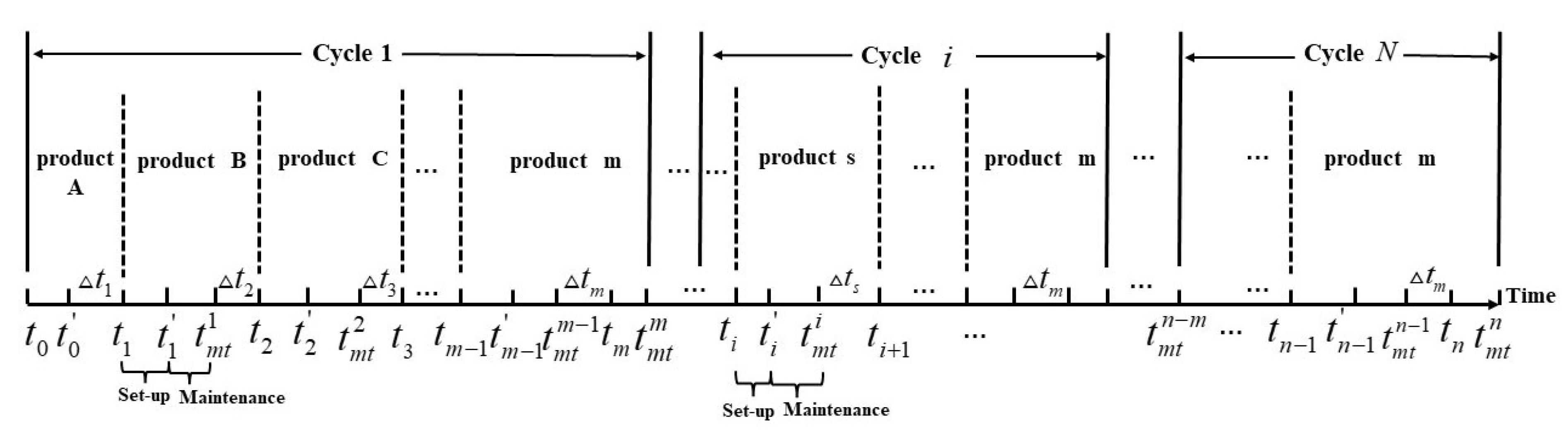
2.2. Maintenance Scheduling

Wireless sensor networks (WSNs) are the key technique in Industrial Internet of Things and modern smart industry [29]. In this paper, we utilize this technique to detect the operational status of this production system and maintenance decisions follow the principle of control constraints. If the magnitude of system degradation does not exceed the pre-defined PM threshold, then no maintenance measures are performed (do nothing). If the magnitude of degradation exceeds the PM threshold but does not exceed the CM threshold, then PM is performed and the system is repaired to a random state between “as new” and “as old”. Otherwise, if the magnitude of degradation exceeds the CM threshold, then CM is performed and the system is repaired to an “as new” state. To facilitate the modelling, this paper assumes that when the magnitude of system degradation reaches the failure threshold, the system does not immediately go down and interrupt the production process, but at this time, it is necessary to perform minimal repair to allow the system to run until the next detection point. In the production process, we do not consider the magnitude of degradation that the system recovers from due to the protection measures.

2.3. Production–Maintenance Interaction

The interaction process between production and condition-based maintenance needs to be described. In a production cycle, the system produces various products in sequence. During this production process, degradation information can be recorded continuously, but maintenance decisions are made only at the intervals of set up based on the state of degradation.
For the sake of clarity, now consider the production in one cycle. The system starts producing each type of product sequentially from the moment t 0 ( t 0 = 0 ). The time period for producing the first product is ( t 0 , t 1 ) and then it is ready to produce the second product until the m - th product is produced. ( t i , t i ) is the set-up time and ( t i , t m t i ) ( i = 0 , 1 , n ) is the maintenance time. This process is shown in Figure 1. If the magnitude of system degradation does not exceed the PM threshold at t i , then neither PM nor CM is taken. If the degradation exceeds the PM threshold but is lower than the CM threshold, then PM is immediate at t i . PM is imperfect in that the degradation level after PM will be reduced to a level below the PM threshold. Otherwise, if the failure threshold is exceeded, a perfect CM is immediate at t i , which will bring the system back to a brand-new state.

2.4. Assumptions

(1)
The demand for all products is fixed and can be divided into small lots for production.
(2)
The production system will produce various products sequentially in a predetermined order.
(3)
Each product is produced only once in a production cycle and the production cycle is a complete run of all products produced according to their lot sizes.
(4)
Inspection time is negligible.
(5)
The magnitude of degradation does not change after the set up.
(6)
During the production process, the magnitude of degradation recovered by the system due to some protective measures is not considered.
(7)
CM results in a fixed cost of loss.
(8)
In case of failure, minimal repairs are always performed without changing the failed process and interrupting the production process.
Assumption 1 is set based on demand-fixed mass production. Assumptions 2 and 3 have already been explained in the system specification. Assumption 4 is an approximation, which is used to simplify the modeling process. In fact, compared with the production time (usually calculated by month or year) and maintenance time (usually calculated by day or month), the inspection time (usually calculated by hour) is much shorter. Assumption 5 is an approximation to practice. In actual production, the system stops running during set up, so the magnitude of degradation does not change. Assumption 6 is to exclude the impact of the system’s protection measures on the degradation magnitude. Assumption 7 is self-setting, because a failure may interrupt the production process and, therefore, cause losses [30]. Assumption 8 is widely used in equipment maintenance modeling [19]. In a typical production industry where recovery from a failure is a very urgent issue, the most economical approach is to repair or replace only the failed component after inspection. Therefore, minimal repairs essentially do not affect the failure rate and intensity of failure in the entire system.

3. Integrated Model

Equipment with nonlinear characteristics of the degradation trajectory is widely available, such as aero-engines [31], milling tools [32], etc. Neglecting the nonlinearity of the degradation process will lead to increased uncertainty in the degradation model [33]. In the last few decades, many degradation models have been proposed in the field of reliability engineering [34,35,36,37,38]. In particular, the degradation of each system element is considered in [38] to model the degradation process. Stochastic process methods are used to evaluate system reliability [39,40]. In order to achieve an accurate description of non-monotonic degenerative processes, the Wiener process began to be introduced into degenerative modeling and has become the most widely used model for stochastic degenerative processes. Since the linear Wiener process is a special form of the nonlinear Wiener process, the nonlinear Wiener process to describe the degradation trajectory of the product has some practical significance and it is more widely used in engineering practice.
According to the nonlinear degradation model of the Wiener process, the X ( t ) = X ( 0 ) + λ Λ ( t , b ) + σ B B ( t ) , X ( t ) denotes the magnitude of degradation in the device performance at time t , λ is a drift coefficient. Λ ( t , b ) is a continuous nonlinear function containing parameters b and time t , which usually has Λ ( t , b ) = t b and Λ ( t , b ) = exp ( b t ) 1 . σ B is the diffusion coefficient, the same value among the same equipment, thus, reflecting the common features among similar products. B ( t ) denotes standard Brownian motion. To not lose generality, make X ( 0 ) = 0 , λ and B ( t ) independent of each other. Assuming that the drift coefficients corresponding to different stages in the same degradation process are constant, it is easy to obtain λ i + 1 = λ i . The Wiener process is an independent incremental process and the degradation increments are Δ X ( Δ t s ) = X ( t i + 1 ) X ( t i ) . It is assumed that the continuous nonlinear function satisfies Λ ( t , b ) = t b and degradation increments Δ X ( Δ t s ) approximate to λ ( t i + 1 b t i b ) , where b is a constant.
For ( t i , t i + 1 ) ( i = 0 , 1 , 2 , m , , n 1 , production of the ( i + 1 ) t h product), assume that the set-up time for each product and the repair time for each degradation state are known, t i + 1 = t m t i + Δ t s , Δ t s is determined by the productivity u and the production lot sizing, Δ t s = Q s / ( N u ) , the s - th ( s = ( i + 1 ) % m ) product should be produced within ( t m t , t i + 1 ) . The total cost from t 0 to t i is C i , the number of PM is r i and the number of CM is f i .

3.1. Maintenance Situations

Depending on whether maintenance actions, either failure-induced or preventive, are conducted at the production set-up points, we conclude the following three situations:
1.
If there is neither CM nor PM at time t i , it means that X ( t i ) < L p , neither PM nor CM is used at this time, so the degradation magnitude does not change either, X ( t m t i ) = X ( t i ) , t m t i = t i . Therefore, the magnitude of degradation at time t i + 1 is X ( t i + 1 ) = X ( t m t i ) + Δ X ( Δ t s ) . At time t i + 1 , there are the following three sub-situations.
(1)
The system has neither CM nor PM: X ( t i + 1 ) = X ( t m t i ) + λ ( t i + 1 b ( t m t i ) b ) < L p . The cost at time t i + 1 is C i + 1 = C i + c i = C i + C m + C s , t m t i + 1 = t i + 1 , no change in the number of PM as r i + 1 = r i , no change in the number of CM as f i + 1 = f i .
(2)
The system performs PM only: L p X ( t i + 1 ) = X ( t m t i ) + λ ( t i + 1 b ( t m t i ) b ) < L f . The cost at time t i + 1 is C i + 1 = C i + Δ c i = C i + C m + C s + C p , t m t i + 1 = t i + 1 + t p m , the number of PM changes to r i + 1 = r i + 1 , no change in the number of CM as f i + 1 = f i .
(3)
The system performs CM only: X ( t i + 1 ) = X ( t m t i ) + λ ( t i + 1 b ( t m t i ) b ) L f . The cost at time t i + 1 is C i + 1 = C i + C m + C s + C f + C l + t s C min , t m t i + 1 = t i + 1 + t c m , the number of CM changes to f i + 1 = f i + 1 , no change in the number of PM as r i + 1 = r i . The minimal repair cost is t s C min , which ensures that the system can continue to operate from t m t i to t i + 1 even though L f is reached in ( t m t i , t i + 1 ) .
2.
If PM is performed at time t i , it means that L p X ( t i ) < L f , the magnitude of degradation at time t m t i after maintenance becomes X ( t m t i ) , which X ( t m t i ) = γ , t m t i = t i + t p m . Here, to ensure the effectiveness of PM, we assume that γ = Φ ( ψ ) L p , Ψ ~ N ( 0 , 1 ) , 1 < ψ < 1 . The magnitude of degradation at time t i + 1 is X ( t i + 1 ) = γ + Δ X ( Δ t s ) . At time t i + 1 , there are the following three sub-situations.
(1)
The system has neither CM nor PM: X ( t i + 1 ) = γ + λ ( t i + 1 b ( t m t i ) b ) < L p . The cost at time t i + 1 is C i + 1 = C i + C m + C s , t m t i + 1 = t i + 1 , no change in the number of PM as r i + 1 = r i , no change in the number of CM as f i + 1 = f i .
(2)
The system performs PM only: L p X ( t i + 1 ) = γ + λ ( t i + 1 b ( t m t i ) b ) < L f . The cost at time t i + 1 is C i + 1 = C i + C m + C s + C p , t m t i + 1 = t i + 1 + t p m . The number of PM changes to r i + 1 = r i + 1 , no change in the number of CM as f i + 1 = f i .
(3)
The system performs CM: X ( t i + 1 ) = γ + λ ( t i + 1 b ( t m t i ) b ) L f . The cost at time t i + 1 is C i + 1 = C i + C m + C s + C f + C l + t s C min , t m t i + 1 = t i + 1 + t c m , the minimal repair cost is t s C min . The number of CM changes to f i + 1 = f i + 1 , no change in the number of PM as r i + 1 = r i .
3.
If CM is performed at time t i , it means that X ( t i ) L f . After maintenance, the magnitude of degradation at time t m t i becomes 0, which is X ( t m t i ) = 0 . The magnitude of degradation at time t i + 1 is X ( t i + 1 ) = X ( t m t i ) + Δ X ( Δ t s ) = λ ( t i + 1 b ( t m t i ) b ) . At time t i + 1 , there are the following three sub-situations.
(1)
The system has neither CM nor PM: X ( t i + 1 ) = λ ( t i + 1 b ( t m t i ) b ) < L p . The cost at time t i + 1 is C i + 1 = C i + C m + C s , t m t i + 1 = t i + 1 , no change in the number of PM as r i + 1 = r i , no change in the number of CM as f i + 1 = f i .
(2)
The system performs PM only: L p X ( t i + 1 ) = λ ( t i + 1 b ( t m t i ) b ) < L f . The cost at time t i + 1 is C i + 1 = C i + C m + C s + C p , t m t i + 1 = t i + 1 + t p m . The number of PM changes to r i + 1 = r i + 1 , no change in the number of CM as f i + 1 = f i .
(3)
The system performs CM: X ( t i + 1 ) = λ ( t i + 1 b ( t m t i ) b ) L f . The cost at time t i + 1 is C i + 1 = C i + C m + C s + C f + C l + t s C min , t m t i + 1 = t i + 1 + t c m , the minimal repair cost is t s C min . The number of CM changes to f i + 1 = f i + 1 , no change in the number of PM as r i + 1 = r i .
The total production and maintenance cost for the integrated model is T C = C n + C H . Inventory holding costs need to be calculated for the entire production and maintenance process. According to the notation and assumptions, the Q s is the demand for the s - th product and N is the number of production cycles (lots). Therefore, we know that the s - th product produces Q s / N in each production cycle and the consumption rate is d s = Q s / [ N s = 1 m ( t s + t s + t m t s ) ] . The maximum inventory of product s - th can be obtained by multiplying the difference between productivity and consumption rate by the production time as ( μ s d s ) t s . Assume that both productivity and consumption rate are fixed, so the total inventory holding rate of product s - th in a production cycle is [ ( s = 1 m t s ) ( μ s d s ) t s ] / 2 . Therefore, we can obtain the total inventory holding cost as C H = N ( i = 1 m t i ) × [ s = 1 m ( μ s d s ) t s C h s ) ] / 2 .
We can obtain the sum of the gross profit of all products
s = 1 m R s Q s
The net profit is
E R = s = 1 m R s Q s T C
Therefore, to maximize the profit per unit time, the optimal decision variables L p and N can be obtained.
U R ( L p , N ) = s = 1 m R s Q s T C N s = 1 m ( t s + t s + t m t s )

3.2. Computation Algorithm for the Model

The calculation algorithm for the model is shown in Algorithm 1. First, determine the approximate range of N and L p , set the initial values of degradation magnitude, time, cost, and maintenance times, and obtain the production time of each product through the actual demand and productivity; then, start production from t = 0 (according to the system specification (detailed description)), in each inspection window and the degradation of the system can be obtained. According to the relationship between the degradation and L p , L f , the type of maintenance the system needs to perform is determined (according to the detailed description of maintenance situations). Calculate and record information, such as the magnitude of degradation after maintenance (or without maintenance), maintenance times, and the maintenance cost and proceed sequentially until the end of production. Finally, it is necessary to traverse all combinations of N and L p to find the combination that maximizes the profit per unit time.
Algorithm 1. Computation algorithm for the model.
1. Give the value range of N and L p .
2. Assign X ( t 0 ) = 0 , t = 0 , T C = 0 , r = 0 , f = 0
3. Obtain Δ t s by Q s / ( u N ) , generate the production time of one cycle.
4. for j = 0 : N
5.  for s = 0 : m
6.   Generate t i based on the required set-up time for each product. Determine which product should be produced at time t m t i .
7.   Determine the maintenance status at time t i based on the degradation quantity X ( t i ) .
8.   Determine the relationship of X ( t i ) with L p and L f , if X ( t i ) < L p , doing nothing, means no repair time. Generate X ( t i + 1 ) from X ( t i ) and Δ X . Obtain the cost C t i + 1 , times of PM r ( t i + 1 ) and times of CM f ( t i + 1 ) at t i + 1 .
9.   else if L p X ( t i ) < L f , carry out PM, need to spend the corresponding PM time, then X ( t i ) into X ( t m t i ) , where X ( t m t i ) = γ . Generate X ( t i + 1 ) from X ( t m t i ) and Δ X . Obtain the cost C t i + 1 , times of PM r ( t i + 1 ) and times of CM f ( t i + 1 ) at t i + 1 .
10.   else X ( t i ) L f , carry out CM, need to spend the corresponding CM time, X ( t i ) into X ( t m t i ) , where X ( t m t i ) = 0 . Generate X ( t i + 1 ) from Δ X . Obtain the cost C t i + 1 , times of PM r ( t i + 1 ) and times of CM f ( t i + 1 ) at t i + 1 .
11.  end
12. end
13. Obtain the total cost T C , total number of PM r , total number of CM f .
14. Calculate profit per unit of time.

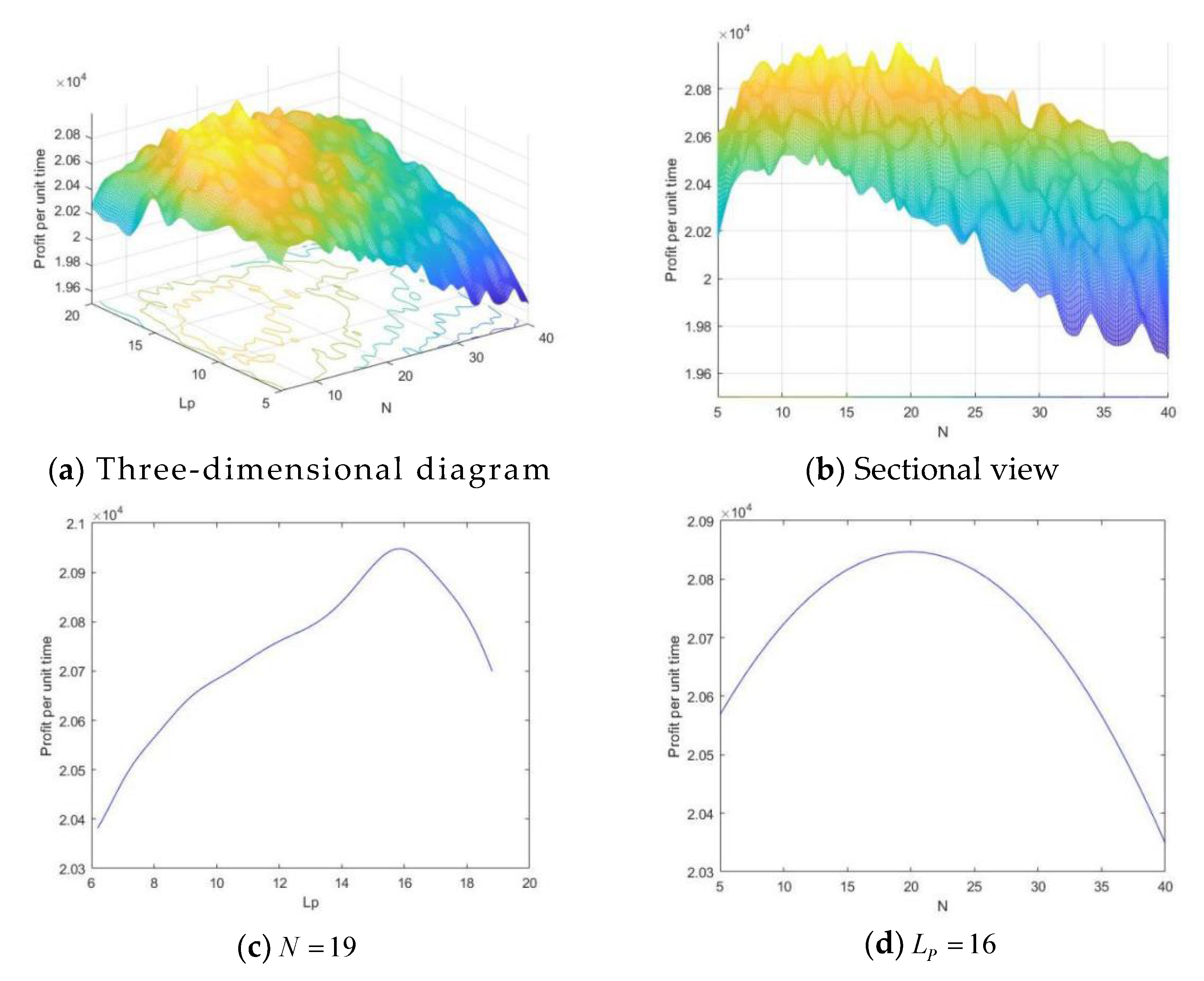
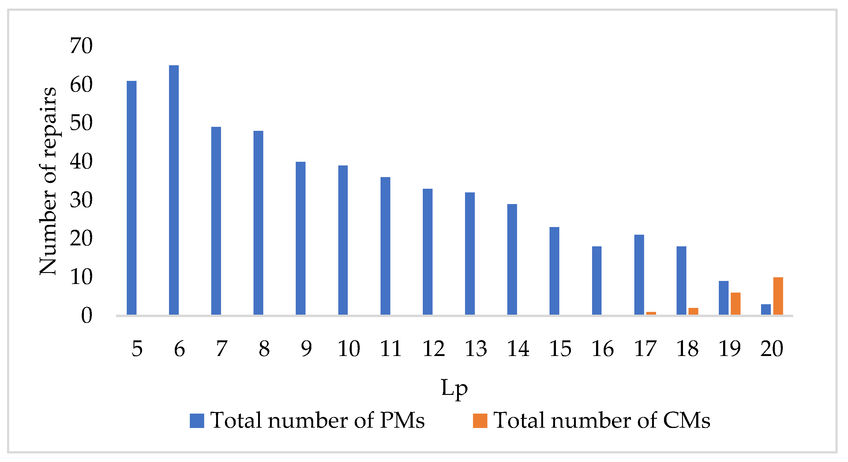
4. Numerical Example

In this section, to verify the validity of the model, we investigate the production of six different sizes of cast iron pipes alternately in a centrifugal system in the literature [19], based on computer simulation principles. Consider this production system in the case of nonlinear degradation and perform production simulation for production lot sizing and PM thresholds. The production equipment is the key equipment in the cast iron process. After preparing the molten iron, the centrifuge is used for casting. The machine stops when different types of cast iron pipes are produced or there is an insufficient supply of molten iron. This is referred to as the make-ready time, which can be used for inspection and maintenance. Production systems may suffer from fatigue cracks, corrosion, and other degradation during the production process. Most of the current manufacturing equipment is complex composite equipment. To simplify the model and allow managers to make generalized decisions, our case studies are not limited to specific components or signals, but monitor the entire production system as a whole.
Since no real data were collected from the production system, we made rough estimates of the parameters based on related work [30], respectively, λ = 0.0458 and b = 1.463 . Different parameters have different effects on system reliability [41]. Although these parameters are not collected from real systems, numerical analysis provides useful insights for analyzing production systems with PM thresholds and production lot sizing.
In this production process, the production quantity is in tons and the unit time is in days. As can be seen from Table 1, the system produces only 6 products, where the minimum demand is 2000. In practice, the number of lot sizing N is less than 100. This indicates that the search space in this case is not very large and the combinatorial optimization method is suitable for solving such optimization problems. In operations research, combinatorial optimization is the process of finding the optimal solution from the solution space to optimize the objective function [42]. Therefore, the combinatorial optimization method is used here to obtain the optimal solution. Assuming the failure threshold L f = 20.5 , the cost parameters are shown in Table 2.
We first programmed the python algorithm to test the performance of the model based on the proposed model and parameter values. The maximum profit per unit of time was 20,997.21. Figure 2 shows the results of the profit per unit time when N goes from 5 to 40 and L P goes from 5 to 20. To clearly illustrate the change in profit per unit time, the results are shown from four perspectives: (a) three-dimensional, (b) sectional view, (c) N = 19 , and (d) L P = 16 .
As can be seen from Figure 2, the profit per unit time rises gradually with different combinations of N and L p , obtaining a maximum value of 20,997.21 at N = 19 and L P = 16 . The results show that the production system can produce 19 production cycles (lots) and the optimal lot sizes for these six products are 4500 / 19 236 , 2500 / 19 131 , 4000 / 19 210 , 3600 / 19 189 , 2000 / 19 105 , 3500 / 19 184 . Excluding maintenance time and set-up time, the duration of a production cycle is approximately 18.9 days.
As shown in Figure 3, it can be seen that when N = 19 , L f = 20.5 , the overall trend of the amount of PM gradually decreases with an increase in L P and the amount of CM gradually increases with an increase in L P . In particular, CM appears only at L P = 17 and it appears more frequently when the value of L P is closer to the value of L f . This can be explained in terms of management logic. For the model in this paper, if the value of L P is set well below the failure threshold L f , then the probability that the magnitude of degradation exceeds L P will increase significantly and PM measures will be implemented more frequently. On the one hand, this will reduce the cost due to CM; on the other hand, the cost of PM will increase as the amount of PM increases and it is likely to cause excessive PM. The profit may be reduced as a result. If the value of L P is set close to the failure threshold L f , then the amount of PM will be significantly reduced and the amount of CM will be obviously increased. This will cause the cost of CM to increase and since CM is much higher than the cost of PM, this will lead to a significant reduction in profit. With the model algorithm in this paper, we can obtain the optimal method to obtain the balance between L P and L f . Thus, determine the value of L P .

5. Conclusions

In this paper, a joint optimization strategy for lot sizing and PM threshold for a nonlinear degenerate multi-product production system was investigated. Based on the degraded state information in the system, a profit maximization model is constructed, a solution algorithm is given, and the validity of the model is illustrated by numerical examples. Compared with the maximum profit obtained by jointly optimizing lot sizing and PM quantity in [20], the minimum cost obtained by jointly optimizing yield and PM interval in [21] and the minimum cost obtained by jointly optimizing the PM strategy and lot sizing in [24], this study illustrates that the maximum profit can be obtained by rationalizing the PM threshold and lot sizing.
The shortcoming of this paper is that the measured value of the performance degradation magnitude is regarded as the real value. In an actual operating environment, due to the interference of external noise, the real performance degradation level in the system is difficult to obtain directly and only the measured value of the performance degradation quantity can be obtained by using condition monitoring means, but there is an error between the measured value and the real value.
On the basis of this study, future research and extensions can be carried out in the following aspects: (1) more in-depth analysis combined with stochastic processes; (2) the model in this paper can also be extended to other degradation systems that can be condition monitored, such as fatigue crack extension, bearing wear, etc.

Author Contributions

Conceptualization, L.Q., J.L. and K.G.; methodology, J.L., K.G. and L.Y.; formal analysis, J.L. and K.G.; investigation, L.Q.; data curation, L.Q., J.L. and K.G.; writing—original draft preparation, L.Q. and J.L.; project administration, L.Q.; funding acquisition, L.Q. and K.G. All authors have read and agreed to the published version of the manuscript.

Funding

This work was funded, in part, by the National Natural Science Foundation of China under Grant 72001027, 72071005 and 72001078, the Chinese Post Doctoral Science Foundation under Grant 270514, and by the R&D Program of Beijing Municipal Education Commission under Grant KM202111232007.

Conflicts of Interest

The authors declare no conflict of interest.

Nomenclature

Abbreviations
PM: Preventive Maintenance
CM: Corrective Maintenance
Notations
N : Production lot sizing
m : The system produces m products in total
Q s : Demand for the s - th product ( s = 1 , 2 , , m )
u s : Productivity of the s - th product
d s : Consumption rate of the s - th product
t : Manufacturing system production time
Δ t s : In a production cycle, the time required to produce the s - th product
t i : The time when the system starts the i + 1 - th set-up ( i = 0 , 1 , m , m + 1 , , n 1 ,   t 0 = 0 )
t i : The time when the system starts the i + 1 - th   maintenance
t s : The s - th product requires a system set-up time
t m t i : The time when the system starts producing the i+1-th product
t m t s : The s - th product requires system maintenance time
C i : Costs incurred in ( t 0 , t i )
Δ c i : Costs incurred in ( t i 1 , t i ) ,   C 1 = Δ c 1
X ( t k ) : The magnitude of degradation of the system at the time t k ( k = 0 , 1 , 2 , m , m + 1 , , n , X ( t 0 ) = 0 )
Δ X : The increment of the degradation magnitude, which is X ( t i + 1 ) X ( t i )
γ : Degradation after PM
L f : CM threshold
L p : PM threshold
r j : The number of PMs performed at the time t j
r : The total number of PMs in the entire production process
f j : The number of CMs at time t j
f : The total number of CMs in the entire production process
%: Remainder sign
C s : The set-up cost of the s - th product
C m : Inspection cost
C min : Average cost of minimal repair
C f : Average cost of a CM cost
C p : Average cost of a PM
C l : The cost of loss caused by a CM
C h s : The average inventory holding cost per unit time of the s - th product
C H : The inventory holding cost of the entire production and maintenance process
T C : The total cost of the entire production and maintenance process
R s : The gross profit of each product, which is equal to the unit sales price minus the unit production cost, excluding maintenance, repair and inventory costs
E R : Net profit
U R : Profit per unit time

References

  1. Peng, R.; Wu, D.; Xiao, H.; Xing, L.; Gao, K. Redundancy versus protection for a non-reparable phased-mission system subject to external impacts. Reliab. Eng. Syst. Saf. 2019, 191, 106556. [Google Scholar] [CrossRef]
  2. Chen, J.; Li, Z. An extended extreme shock maintenance model for a deteriorating system. Reliab. Eng. Syst. Saf. 2017, 93, 1123–1129. [Google Scholar] [CrossRef]
  3. Rafiee, K.; Feng, Q.; Coit, D.W. Condition-Based Maintenance for Repairable Deteriorating Systems Subject to a Generalized Mixed Shock Model. IEEE Trans. Reliab. 2015, 64, 1164–1174. [Google Scholar] [CrossRef]
  4. Ye, Z.-S.; Wang, Y.; Tsui, K.-L.; Pecht, M. Degradation data analysis using wiener processes with measurement errors. IEEE Trans. Reliab. 2013, 62, 772–780. [Google Scholar] [CrossRef]
  5. Zeng, S.W. General model for analysis of manufacturing cost, reliability, availability and maintenance in manufacturing systems. In Proceedings of the 9th International Conference on Reliability and Maintainability, La Baule, France, 30 May–3 June 1994; pp. 260–275. [Google Scholar]
  6. Pandey, M.; Zuo, M.J.; Moghaddass, R.; Tiwari, M. Selective maintenance for binary systems under imperfect repair. Reliab. Eng. Syst. Saf. 2013, 113, 42–51. [Google Scholar] [CrossRef]
  7. Yang, L.; Li, G.; Zhang, Z.; Ma, X.; Zhao, Y. Operations & Maintenance Optimization of Wind Turbines Integrating Wind and Aging Information. IEEE Trans. Sustain. Energy 2020, 12, 211–221. [Google Scholar] [CrossRef]
  8. Zhang, Z.; Yang, L. State-based opportunistic maintenance with multifunctional maintenance windows. IEEE Trans. Reliab. 2020, 70, 1481–1494. [Google Scholar] [CrossRef]
  9. Sun, Q.; Ye, Z.-S.; Peng, W. Scheduling Preventive Maintenance Considering the Saturation Effect. IEEE Trans. Reliab. 2018, 68, 741–752. [Google Scholar] [CrossRef]
  10. de Jonge, B.; Scarf, P.A. A review on maintenance optimization. Eur. J. Oper. Res. 2019, 285, 805–824. [Google Scholar] [CrossRef]
  11. Jardine, A.K.; Lin, D.; Banjevic, D. A review on machinery diagnostics and prognostics implementing condition-based maintenance. Mech. Syst. Signal Process. 2006, 20, 1483–1510. [Google Scholar] [CrossRef]
  12. Mann, L.; Saxena, A.; Knapp, G.M. Statistical-based or condition-based preventive maintenance? J. Qual. Maint. Eng. 1995, 1, 46–59. [Google Scholar] [CrossRef]
  13. Huynh, K.; Barros, A.; Bérenguer, C.; Castro, I. A periodic inspection and replacement policy for systems subject to competing failure modes due to degradation and traumatic events. Reliab. Eng. Syst. Saf. 2011, 96, 497–508. [Google Scholar] [CrossRef]
  14. Ahmad, R.; Kamaruddin, S. An overview of time-based and condition-based maintenance in industrial application. Comput. Ind. Eng. 2012, 63, 135–149. [Google Scholar] [CrossRef]
  15. Chen, H.; Yan, X.; Zhang, Y.; Niu, X. A review of production system maintenance management-statistical process control-economic production lot integration optimization research. Mod. Manuf. Eng. 2020, 10, 148–155+12. (In Chinese) [Google Scholar] [CrossRef]
  16. Gao, K.; Yan, X. Study on the Optimal Strategy of Missile Interception. IEEE Access 2021, 9, 22239–22252. [Google Scholar] [CrossRef]
  17. Weinstein, L.; Chung, C.-H. Integrating maintenance and production decisions in a hierarchical production planning environment. Comput. Oper. Res. 1999, 26, 1059–1074. [Google Scholar] [CrossRef]
  18. Aghezzaf, E.H.; Jamali, M.A.; Ait-Kadi, D. An integrated production and preventive maintenance planning model. Eur. J. Oper. Res. 2007, 181, 679–685. [Google Scholar] [CrossRef]
  19. Hajej, Z.; Rezg, N.; Gharbi, A. Joint optimization of production and maintenance planning with an environmental impact study. Int. J. Adv. Manuf. Technol. 2017, 93, 1269–1282. [Google Scholar] [CrossRef]
  20. Gao, K.; Peng, R.; Qu, L.; Wu, S. Jointly optimizing lot sizing and maintenance policy for a production system with two failure modes. Reliab. Eng. Syst. Saf. 2020, 202, 106996. [Google Scholar] [CrossRef]
  21. Liu, X.; Wang, W.; Zhang, T.; Zhai, Q.; Peng, R. An integrated production, inventory and preventive maintenance model for a multi-product production system. Reliab. Eng. Syst. Saf. 2015, 137, 76–86. [Google Scholar] [CrossRef]
  22. Bouslah, B.; Gharbi, A.; Pellerin, R. Integrated production, sampling quality control and maintenance of deteriorating production systems with AOQL constraint. Omega 2016, 61, 110–126. [Google Scholar] [CrossRef]
  23. Peng, H.; van Houtum, G.-J. Joint optimization of condition-based maintenance and production lot-sizing. Eur. J. Oper. Res. 2016, 253, 94–107. [Google Scholar] [CrossRef]
  24. Jafari, L.; Makis, V. Joint optimal lot sizing and preventive maintenance policy for a production facility subject to condition monitoring. Int. J. Prod. Econ. 2015, 169, 156–168. [Google Scholar] [CrossRef]
  25. Jafari, L.; Makis, V. Optimal lot-sizing and maintenance policy for a partially observable production system. Comput. Ind. Eng. 2016, 93, 88–98. [Google Scholar] [CrossRef]
  26. Sarker, R.; Haque, A. Optimization of maintenance and spare provisioning policy using simulation. Appl. Math. Model. 2000, 24, 751–760. [Google Scholar] [CrossRef]
  27. Zhao, X.; Chai, X.; Sun, J. Joint optimization of mission abort and component switching policies for multistate warm standby systems. Reliab. Eng. Syst. Saf. 2021, 212, 107641. [Google Scholar] [CrossRef]
  28. Qiu, Q.; Maillart, L.; Prokopyev, O.; Cui, L. Optimal Condition-Based Mission Abort Decisions. IEEE Trans. Reliab. 2022, 5, 1–18. [Google Scholar] [CrossRef]
  29. Gao, K.; Peng, R.; Qu, L.; Xing, L.; Wang, S.; Wu, D. Linear system design with application in wireless sensor networks. J. Ind. Inf. Integr. 2021, 27, 100279. [Google Scholar] [CrossRef]
  30. Gao, K.; Yan, X.; Peng, R.; Xing, L. Economic Design of a Linear Consecutively Connected System Considering Cost and Signal Loss. IEEE Trans. Syst. Man Cybern. Syst. 2019, 51, 5116–5128. [Google Scholar] [CrossRef]
  31. Guo, Q.; Li, Y.; Zheng, T. Prediction of aero-engine performance degradation based on nonlinear Wiener process. Propuls. Technol. 2021, 42, 1956–1963. (In Chinese) [Google Scholar]
  32. Goebel, K.; Agogino, A. Mill data set [DB/OL]. In NASA. Available online: http://ti.arc.nasa.gov/project/prognostic-data-repository (accessed on 15 April 2022).
  33. Wang, Z.; Chen, Y.; Cai, Z.; Luo, C. Residual life prediction considering nonlinear degradation with stochastic failure threshold. J. Natl. Univ. Def. Technol. 2020, 42, 177–185. (In Chinese) [Google Scholar]
  34. Li, Y.-F.; Zio, E.; Lin, Y.-H. A Multistate Physics Model of Component Degradation Based on Stochastic Petri Nets and Simulation. IEEE Trans. Reliab. 2012, 61, 921–931. [Google Scholar] [CrossRef]
  35. Gebraeel, N.; Elwany, A.; Pan, J. Residual Life Predictions in the Absence of Prior Degradation Knowledge. IEEE Trans. Reliab. 2009, 58, 106–117. [Google Scholar] [CrossRef]
  36. Giorgio, M.; Guida, M.; Pulcini, G. An age- and state-dependent Markov model for degradation processes. IIE Trans. 2011, 43, 621–632. [Google Scholar] [CrossRef]
  37. Kim, M.J.; Makis, V. Optimal maintenance policy for a multi-state deteriorating system with two types of failures under general repair. Comput. Ind. Eng. 2009, 57, 298–303. [Google Scholar] [CrossRef]
  38. Yi, K.; Kou, G.; Gao, K.; Xiao, H. Optimal allocation of multi-state elements in a sliding window system with phased missions. J. Risk Reliab. 2020, 235, 50–62. [Google Scholar] [CrossRef]
  39. Gao, K. Simulated Software Testing Process and Its Optimization Considering Heterogeneous Debuggers and Release Time. IEEE Access 2021, 9, 38649–38659. [Google Scholar] [CrossRef]
  40. Lei, B.; Gao, K.; Yang, L.; Fang, S. A Model of Optimal Interval for Anti-Mosquito Campaign Based on Stochastic Process. Mathematics 2022, 10, 440. [Google Scholar] [CrossRef]
  41. Huang, S.; Lei, B.; Gao, K.; Wu, Z.; Wang, Z. Multi-State System Reliability Evaluation and Component Allocation Optimization Under Multi-Level Performance Sharing. IEEE Access 2021, 9, 88820–88834. [Google Scholar] [CrossRef]
  42. Gao, K.; Xiao, H.; Qu, L.; Wang, S. Optimal interception strategy of air defence missile system considering multiple targets and phases. Proc. Inst. Mech. Eng. Part O J. Risk Reliab. 2021, 236, 138–147. [Google Scholar] [CrossRef]
Figure 1. Production and maintenance process.
Applsci 12 08638 g001
Figure 2. The profit per unit time as a function of N and L p by the model.
Applsci 12 08638 g002
Figure 3. When N = 19 , L p corresponds to the number of repairs.
Applsci 12 08638 g003
Table 1. Different parameter values of different products.
Product Q u C s C h s R s
14500502000.31380
22500502100.53410
34000802050.42400
43600602000.55380
52000502200.34420
63500502080.52400
Table 2. Same parameter values of different products.
C M C p C f C l C min
10050050001000200
Publisher’s Note: MDPI stays neutral with regard to jurisdictional claims in published maps and institutional affiliations.

