Reliability Modelling Considering Self-Exciting Mechanisms of Shock Damage

Abstract

This study investigates reliability modelling and optimal preventive maintenance polices for engineering systems subject to shocks, considering two types of self-exciting mechanisms. Under trigger mechanism 1, if the accumulative number of $\delta$—ineffective shocks reaches the trigger threshold $k_1$ among the run of ineffective shocks, then the self-exciting mechanism will be activated, resulting in the accumulative number of effective shocks increasing by $m_1$. Under trigger mechanism 2, if the consecutive number of $\delta$—ineffective shocks reaches a fixed threshold K₂ among the run of ineffective shocks, then the self-exciting mechanism will be triggered and the accumulative number of effective shocks will increase by $m_2$. The system breaks down when the accumulative number of effective shocks exceeds the fixed threshold. Based on the established shock models, the reliability indices are obtained through the finite Markov chain imbedding approach. According to the operation of the system under different monitoring conditions, two types of preventive maintenance strategies are considered; then, optimization models are established, and the optimal preventive maintenance thresholds are determined. Finally, the proposed models are illustrated by numerical examples.

1. Introduction

Internal deterioration and external shock damage are two main sources of system failure, and the shock model is commonly applied to characterize the impact of external damage on system failure behavior such as overload and vibration. Shock models have received extensive attention both theoretically and practically [1,2]. Numerous shock models have been established during the past few decades and can be divided into five basic categories: accumulative shock [3], extreme shock [4], run shock [5], $\delta$—shock [6] and mixed shock [7]. In the accumulative shock model, system failure is due to the accumulative effect. Under the extreme impact model, the system will collapse as long as the single impact exceeds the critical value. The system breaks down when $k$ consecutive shocks arrive and the magnitude exceeds the failure threshold. In the $\delta$—shock model, when the time interval between two adjacent shocks is smaller than a fixed threshold, the system will malfunction. In addition, shock models can be combined to construct a mixed shock model [8].

Existing research on shock models are mainly focused on reliability evaluation and optimal preventive maintenance strategy. In reliability engineering, system reliability, survival rate and failure rate function are discussed extensively. Zhao et al. [9] studied the reliability modelling and optimal triggering policy of protective devices for multi-state systems subject to shocks. Zhao et al. [10] established mixed two-stage shock models governed by a run of external shocks with certain lengths. Wang et al. [11] applied the copula function in deriving the joint distribution of dependent deterioration processes. Li et al. [12] proposed reliability models for phased mission systems with finite and infinite random shocks and compared the evaluated system reliability under different shock modes. Yang et al. [13] studied condition based maintenance strategy for redundant systems subject to shock damage using improved reinforcement learning. Lin et al. [14] considered the system reliability with both internal deterioration and external damage and used the Monte Carlo simulation to evaluate the system reliability. In addition, some results of reliability analyses of shock models have also been studied [15,16,17,18,19].

For systems operating in a shock environment, designing appropriate maintenance policies is crucial for mitigating the failure risk caused by external shock damage. Chang et al. [20] proposed a maintenance policy where the system is removed by a minimal repair when experiencing a type-I failure and a perfect repair when experiencing a type-II failure; then, a hybrid replacement policy is possible, considering system age, failure modes, and repair cost. Qiu et al. [21] studied an optimal preventive maintenance policy for systems subject to shock damage modelled by the shot noise process. Nakagawa [22] introduced a replacement policy to replace an element when the total damage exceeds the critical threshold. Zhao et al. [23] put forward three preventive maintenance strategies for systems with varying monitoring conditions, and optimization models were formulated to determine the optimal maintenance thresholds. Zhao et al. [24] proposed novel shock models to characterize the case that the component damage process will be accelerated with the increase of the damage degree in a shock environment. Wang et al. [25] described the deterioration and shock processes of the traction power supply system by the jump process and developed a preventive maintenance strategy to minimize the average cost rate. Yang et al. [26] proposed a condition-based maintenance policy for systems subject to internal degradation and external damage and evaluated the average cost per unit time by jointly optimizing the preventive thresholds and the periodic inspection frequency. Other operations and maintenance strategies in a shock environment have been reported [27,28,29,30].

In addition to performing preventive maintenance, self-healing ability has recently emerged as another effective way to enhance the system reliability, due to the rapid development of technology. To evaluate the system reliability with consideration of self-healing mechanisms existing in polymer matrix composite materials, Liu et al. [31] characterize healing time and healing level in the self-healing process of shocks. Cha et al. [32] suggested a new type of shock models, where each delayed failure can be cured with certain probabilities. Cui et al. [33] developed accumulative damage shock models and introduced the concept of self-healing effects.

As another special mechanism in terms of shock damage, the damage self-exciting phenomenon, is also commonly observed in various engineering fields. For example, an aircraft with self-exciting materials may encounter turbulence that causes some damage to the fuselage. When the accumulative external shock damage exceeds the critical threshold, the aircraft will fail and cause extreme losses. If there is no effective shock in a time period, and the airframe suffers some appropriate stimulation, the self-exciting mechanism can be triggered. These stimuli can be considered as ineffective shocks and can be heat, light or electric fields. As another example, a software module includes a string of codes. The errors in software can result in software failure. We can consider the ‘bugs’ as a kind of shock and the software failure means the answers generated by the software are deviant from required answer. If there is no effective impact in a period of time and some ineffective bugs occur, then the self-exciting phenomenon will appear.

Due to its significant impact on system failure behavior, the self-exciting phenomenon should be given full consideration in system reliability evaluation. Anastasia Borovykh et al. [34] considered that reserves are subjected to self-exciting and cross-exciting shocks and proposed a modelling method. Chen et al. [35] proposed approaches to model reliability growth and provided a common evaluation method to model self-exciting point processes. Wang et al. [36] established a model considering mixed shock models and self-exciting mechanisms to generalize software reliability models.

Despite the popularity of the self-exciting phenomenon, little research has been dedicated to the reliability modelling of the self-exciting process in a shock environment. Although the proposed model shares some similarities with Zhao et al. [23], we extend the research by considering two novel self-exciting triggering mechanisms. To be specific, Zhao et al. [23] proposed a self-healing mechanism by considering that the damage caused by a valid shock can be healed when the number of invalid shocks reaches a threshold in the trailing run of invalid shocks. In contrast, we propose two novel self-exciting mechanisms by considering that the effective shocks are increased when the number of ineffective shocks attain the trigger threshold. Two types of self-exciting trigger mechanisms are considered based on the consecutive and cumulative number of ineffective shocks. To this end, this paper develops novel shock models considering two types of self-exciting triggering mechanisms. Under trigger mechanism 1, when the accumulative number of $\delta$—ineffective shocks reaches the trigger threshold $k_1$ among the run of ineffective shocks, the system will trigger the self-exciting mechanism, and the accumulative number of effective shocks will increase by $m_1$. Under trigger mechanism 2, when the consecutive number of $\delta$—ineffective shocks reaches the trigger threshold $k_2$ among the run of ineffective shocks, the system will trigger the self-exciting mechanism, and the accumulative number of effective shocks will increase by $m_2$. Based on the established shock models, we analyze the system reliability. Two maintenance policies are proposed, considering different monitoring conditions to minimize the average cost rate.

The remainder of the paper is organized as follows. Section 2 establishes shock models under two self-exciting trigger mechanisms. Section 3 evaluates the system reliability under two models. Two types of maintenance strategies are proposed, and the optimal maintenance policies are established to minimize the average long-term cost rate in Section 4. Numerical examples are given in Section 5. Finally, the conclusions and future research are presented in Section 6.

2. Model Assumptions and Model Description

Problem Description

The system considered operates in a stochastic environment modeled by a homogeneous Poisson impact process. The time lag between adjacent shocks is independent and identically distributed following exponential distribution with parameter $\lambda$. Arrived shocks can be classified as effective shocks, with probability $p$ that can lead to system damage, and ineffective shocks, with probability $1-p$, which are harmless to the system. When the accumulative number of effective shocks exceeds the threshold $n$, the system will fail. When the time interval between an ineffective shock and the previous shock is less than the given threshold $\delta$, it is defined as an $\delta$—ineffective shock. When the arrival of shocks is more frequent, the self-exciting mechanism is triggered, and the accumulative number of effective shocks will increase by a certain number. Two types of self-exciting mechanisms are considered.

Trigger mechanism 1: Under this trigger mechanism, among the run of ineffective shocks, when the accumulative number of $\delta$—ineffective shocks reaches $k_1$, the self-exciting mechanism will be triggered to increase the accumulative number of effective shocks by $m_1$.

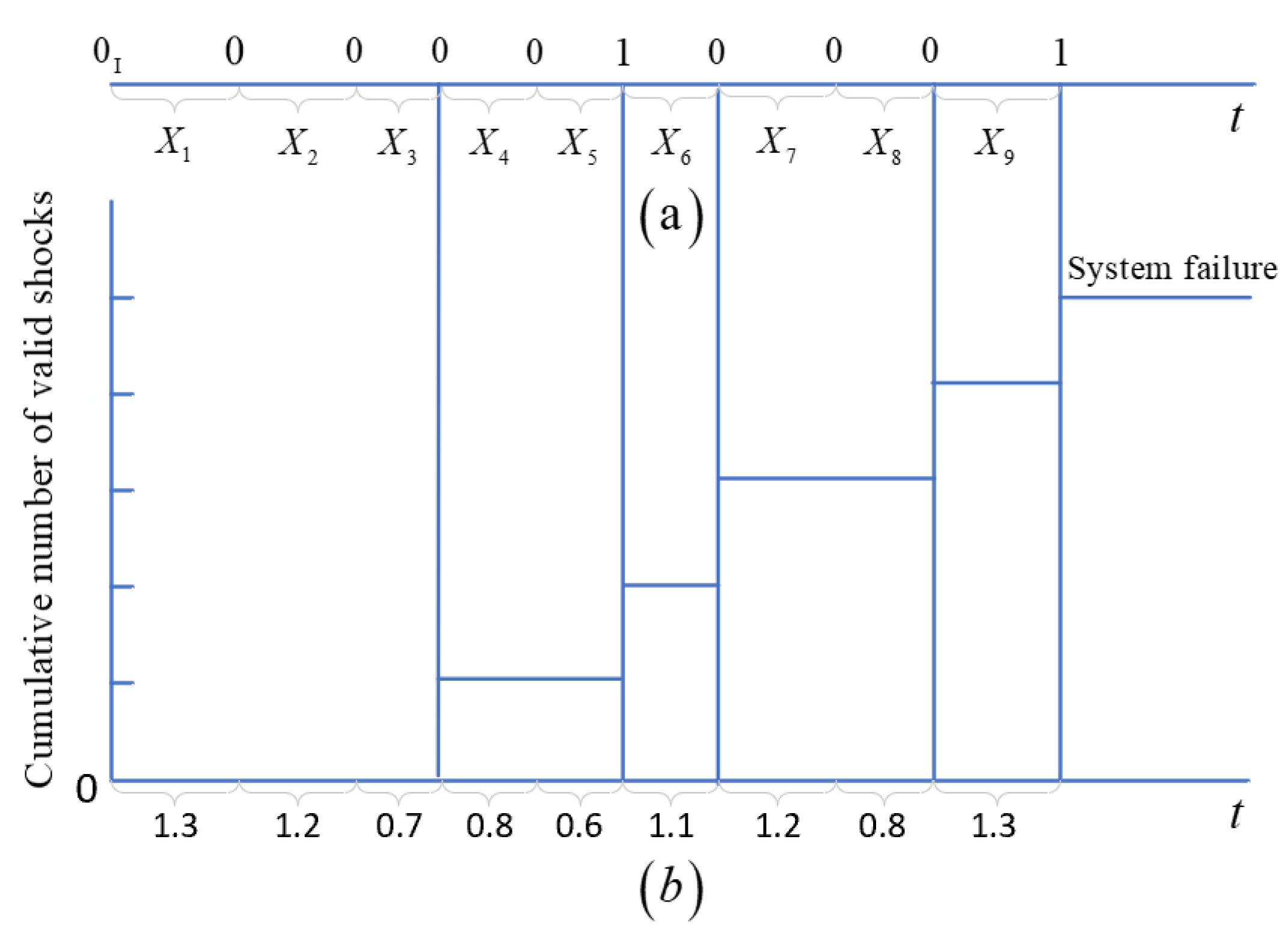
Let $X_i,i=1,2,\dots$ indicate the time lag between the (i − 1)th and ith shock. Figure 1 shows the possible evolution of the system failure process under trigger mechanism 1, where $n=5$, $k_1=2$, $\delta =1.25$, $m_1=1$. Let ‘$1$’ denote effective shocks, ‘$0$’ denote ineffective shocks, and ‘$0_{\mathrm{I}}$’ denote the initial state of the shock sequence. In Figure 1a, the first four shocks are $\delta$—ineffective shocks. Figure 1b shows the corresponding accumulative number of effective shocks. Upon the 3rd shock, the accumulative number of $\delta$—ineffective shocks in the trailing run of ineffective shock reaches 2, then the self-exciting mechanism will be triggered and the accumulative number of effective shocks increases by 1. In the same way, when the 6th shock occurs, the accumulative number of ineffective shocks in the trailing run of $\delta$—ineffective shocks reaches 2, the self-exciting mechanism is triggered again, and the accumulative number of effective shocks increases by 1. When the 9th shock occurs, the accumulative number of effective shocks reaches 5, and the system fails.

Trigger mechanism 2: Under this trigger mechanism, among the run of ineffective shocks, when the consecutive number of $\delta$—ineffective shocks reaches $k_2$, the self-exciting mechanism is triggered to increase the accumulative number of effective shocks by $m_2$.

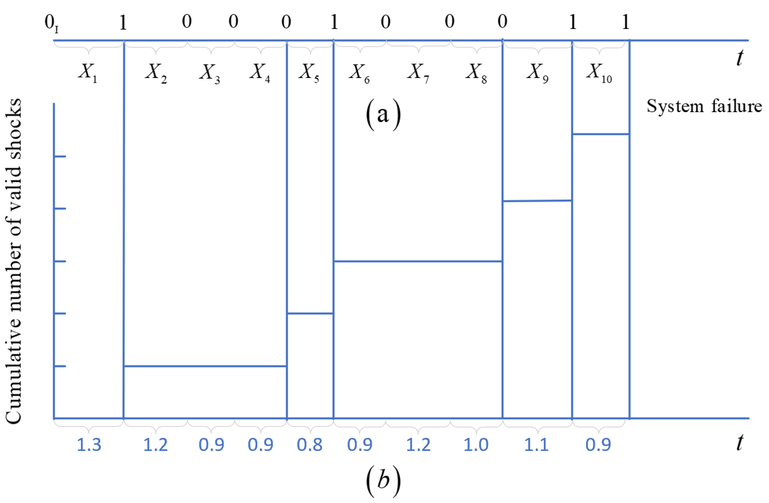
Figure 2 shows the failure process of the system, where $n=5$, $k_2=3$, $\delta =1.25$, and $m_2=1$. When the 4th shock occurs, the accumulative number of $\delta$—ineffective shocks in the trailing run of ineffective shock reaches 2; then, the self-exciting mechanism will be triggered, and the accumulative number of effective shocks should be increased by 1. When the 4th shock occurs, the consecutive number of ineffective shocks in the trailing run of ineffective shocks is three, so the self-exciting mechanism is triggered. When the 8th shock occurs, the consecutive number of $\delta$—ineffective shocks in the trailing run of ineffective shocks reaches 2, the self-exciting mechanism is triggered, and the accumulative number of effective shocks should be increased by 1. When the 10th shock occurs, the accumulative effective shock times of the system reaches 5, and the system fails.

3. Reliability Modelling and Evaluation

3.1. Reliability Modelling and Evaluation under Triggering Mechanism 1

In this section, we use the finite Markov chain imbedding method to conduct probabilistic analysis under triggering mechanism 1.

First, we define three random variables in the sequence of $h_1$ random shocks. Let $U_{h_1}$ denote the accumulative number of effective shocks. Let $V_{h_1}$ represent the number of $\delta$—ineffective shocks in the trailing run of ineffective shocks. Let $W_{h_1}$ denote the number of $\delta$—ineffective shocks that can trigger the next self-exciting mechanism, where $W_{h_1}=V_{h_1}-\left[\frac{V_{h_1}}{k_1}\right]·k_1$, $\left[\frac{V_{h_1}}{k_1}\right]$ is the integer part of $\frac{V_{h_1}}{k_1}$.

A Markov chain $\left\{Y_{h_1},h_1\ge 0\right\}$ that is associated with $U_{h_1}$ and $W_{h_1}$ is defined as $Y_{h_1}=\left(U_{h_1},W_{h_1}\right)$, for $h_1\ge 0$. The state space is ${\mathsf{\Omega }}_1=\left\{\left(u_1,w_1\right):0\le u_1\le n_1-1\right\}\cup \left\{E_a\right\}$. Let $Y_{h_1}=\left(u_1,w_1\right)$ denote that the system has been impacted $h_1$ times.

Let $u_1$ denote the accumulative number of effective shocks. Let $w_1$ denote the number of $\delta$—ineffective shocks that can trigger the next self-exciting mechanism. Let $Y_0=\left(0,0\right)$ denote the initial state. Let $E_a$ denote the absorbing state where the accumulative number of effective shocks reaches $n$ and the system fails.

Let $q_1$ denote the probability that the $h_1-\mathrm{th}$ shock is a $\delta$—ineffective shock whose time lag with the preceding shock is less than $\delta$. Let $q_2$ denote the probability that the $h_1-\mathrm{th}$ shock is an ineffective shock whose time lag with the preceding shock exceeds $\delta$, where $q_1=q·P\left\{X_m<\delta \right\}$, $q_2=q·P\left\{X_m\ge \delta \right\}$ and $q_1+q_2=q$.

Table 1. Transition probabilities in ${\mathsf{\Lambda }}_1$.

No.	Applicability	Condition	Prob.
1	$0\le u_1<n-1,0\le w_1<k_1-1$	$P\left\{Y_{h_1}=\left(u_1,w_1\right)|Y_{h_1-1}=\left(u_1,w_1\right)\right\}$	$q_2$
2	$0\le u_1<n-1,0\le w_1<k_1-1$	$P\left\{Y_{h_1}=\left(u_1+1,0\right)|Y_{h_1-1}=\left(u_1,w_1\right)\right\}$	$p$
3	$0\le u_1<n-1,0\le w_1<k_1-1$	$P\left\{Y_{h_1}=\left(u_1,w_1+1\right)|Y_{h_1-1}=\left(u_1,w_1\right)\right\}$	$q_1$
4	$0\le u_1<n-1,w_1=k_1-1$	$P\left\{Y_{h_1}=\left(u_1,w_1\right)|Y_{h_1-1}=\left(u_1,w_1\right)\right\}$	$q_2$
5	$0\le u_1<n-1,w_1=k_1-1$	$P\left\{Y_{h_1}=\left(u_1+1,0\right)|Y_{h_1-1}=\left(u_1,w_1\right)\right\}$	$p+q_1$
6	$u_1=n-1,0\le w_1<k_1-1$	$P\left\{Y_{h_1}=\left(u_1,w_1\right)|Y_{h_1-1}=\left(u_1,w_1\right)\right\}$	$q_2$
7	$u_1=n-1,0\le w_1<k_1-1$	$P\left\{Y_{h_1}=E_a|Y_{h_1-1}=\left(u_1,w_1\right)\right\}$	$p$
8	$u_1=n-1,0\le w_1<k_1-1$	$P\left\{Y_{h_1}=\left(u_1,w_1+1\right)|Y_{h_1-1}=\left(u_1,w_1\right)\right\}$	$q_1$
9	$u_1=n-1,w_1=k_1-1$	$P\left\{Y_{h_1}=\left(u_1,w_1\right)|Y_{h_1-1}=\left(u_1,w_1\right)\right\}$	$q_2$
10	$u_1=n-1,w_1=k_1-1$	$P\left\{Y_{h_1}=E_a|Y_{h_1-1}=\left(u_1,w_1\right)\right\}$	$p+q_1$
11	$n/a$	$P\left\{Y_{h_1}=E_a|Y_{h_1-1}=E_a\right\}$	1
12	$n/a$	Others	0

shows the transition rules of the transition probability matrix ${\mathsf{\Lambda }}_1$ of Markov chain $\left\{Y_{h_1},h_1\ge 0\right\}$.

For example, when $n=4$, $k_1=2$, $m_1=1$, the state space ${\mathsf{\Omega }}_1$ for the Markov chain $\left\{Y_{h_1},h_1\ge 0\right\}$ is constructed as

$${\mathsf{\Omega }}_1=\left\{\left(0,0\right),\left(0,1\right),\left(1,0\right),\left(1,1\right),\left(2,0\right),\left(2,1\right),\left(3,0\right),\left(3,1\right)\right\}\cup \left\{E_a\right\}$$

Based on the transition rules, we can obtain the one-step transition probability matrix:

$${\mathsf{\Lambda }}_1=\begin{array}{c}\left(0,0\right)\\ \left(0,1\right)\\ \left(1,0\right)\\ \left(1,1\right)\\ \left(2,0\right)\\ \left(2,1\right)\\ \left(3,0\right)\\ \left(3,1\right)\\ E_a\end{array}{\left[\begin{array}{ccccccccc}{q}_2& q_1& p& 0& 0& 0& 0& 0& 0\\ 0& q_2& p+q_1& 0& 0& 0& 0& 0& 0\\ 0& 0& q_2& q_1& p& 0& 0& 0& 0\\ 0& 0& 0& q_2& p+q_1& 0& 0& 0& 0\\ 0& 0& 0& 0& q_2& q_1& p& 0& 0\\ 0& 0& 0& 0& 0& q_2& p+q_1& 0& 0\\ 0& 0& 0& 0& 0& 0& q_2& q_1& p\\ 0& 0& 0& 0& 0& 0& 0& q_2& p+q_1\\ 0& 0& 0& 0& 0& 0& 0& 0& 1\end{array}\right]}_{9\times 9}.$$

The transition probability matrix ${\mathsf{\Lambda }}_1$ with order ${\gamma }_1$ can be partitioned into four submatrices:

$${\mathsf{\Lambda }}_1=\left[\begin{array}{cc}{\mathbf{P}}_{1_{\left(\gamma -1\right)\times \left(\gamma -1\right)}}& {\mathbf{Q}}_{1_{\left(\gamma -1\right)\times 1}}\\ {\mathbf{0}}_{1_{1\times \left(\gamma -1\right)}}& {\mathbf{E}}_{1_{1\times 1}}\end{array}\right],$$

where ${\mathbf{P}}_{1_{\left(\gamma -1\right)\times \left(\gamma -1\right)}}$ is a transition probability matrix between each transient state, ${\mathbf{Q}}_{1_{\left(\gamma -1\right)\times 1}}$ is the column matrix from each transient state to the absorption state, ${\mathbf{0}}_{1_{1\times \left(\gamma -1\right)}}$ is a zero matrix, which is the transition probability matrix from the absorption state to transient state, and ${\mathbf{E}}_{1_{1\times 1}}$ is an identity matrix representing the probability from the absorption state to the absorption state.

Let $N_1$ denote the total number of shocks before the system failure. We can derive some probabilistic indices related to the shock numbers $N_1$ by the following equations. The distribution function of the shock numbers $N_1$ is

$$P\left\{N_1\le l\right\}={\displaystyle \sum _{j=1}^l{\mathsf{\alpha }}_1{\mathbf{P}}_1{}^{j-1}}{{\mathbf{e}}^{\prime }}_1{}_{{}_{\gamma -1}}=1-{\mathsf{\alpha }}_1{\mathbf{P}}_1{}^l{{\mathbf{e}}^{\prime }}_1{}_{{}_{\gamma -1}},$$

(1)

where ${\mathsf{\alpha }}_1={\left(1,0,\dots ,0\right)}_{1\times \left(\gamma -1\right)},$ and ${\mathbf{e}}_1{}_{{}_{\gamma -1}}={\left(1,\dots ,1\right)}_{1\times \left(\gamma -1\right)}.$

The probability mass function of the shock numbers $N_1$ is

$$P\left\{N_1=l\right\}={\mathsf{\alpha }}_1{\mathbf{P}}_1{}^{l-1}{\mathbf{Q}}_1.$$

(2)

The expected number of shocks $E\left(N_1\right)$ is

$$E\left(N_1\right)={\alpha }_1{\left(I_1-P_1\right)}^{-1}{{\mathbf{e}}^{\prime }}_1{}_{{}_{\gamma -1}}.$$

(3)

We can derive the probability density function of $T$ when $N_1=n$:

$$f_1\left(t\right)=\{\begin{array}{cc}{\lambda }^n{t}^{n-1}\exp \left(-\lambda t\right)/\left(n-1\right)!,& t\ge 0\\ 0,& t<0.\end{array}$$

(4)

In addition, we can obtain the probability density function of $T$ by using the Law of Total Probability:

$$f_1\left(t\right)=\{\begin{array}{cc}{\displaystyle \sum _{l=1}^{\infty }\left[\left({\lambda }^l{t}^{l-1}\exp \left(-\lambda t\right)/\left(l-1\right)!\right)\times P\left\{N_1=l\right\}\right]},& t\ge 0\\ 0,& t<0.\end{array}$$

(5)

The expected system life $E\left(T_1\right)$ is

$$E\left(T_1\right)={\displaystyle \underset{0}{\overset{\infty }{\int }}t{f}_1\left(t\right)}dt$$

(6)

Then, we can show the reliability function of the system as

$$\begin{array}{ll}{R}_1\left(x\right)& =P\left\{T>x\right\}\\ & =P\left\{{\displaystyle \sum _{i=1}^{N_1}{X}_i>x}\right\}\\ & =1-{\displaystyle {\int }_0^x{\displaystyle \sum _{l=1}^{\infty }\left[\left({\lambda }^l{t}^{l-1}\exp \left(-\lambda t\right)/\left(l-1\right)!\right)\times P\left\{N_1=l\right\}\right]}dt}.\end{array}$$

(7)

3.2. Reliability Modelling and Evaluation under Trigger Mechanism 2

In this section, we use the finite Markov chain imbedding method to conduct probabilistic analysis under trigger mechanism 2.

First, we define three random variables in the sequence of $h_1$ random shocks. Let $U_{h_2}$ denote the accumulative number of effective shocks.

Let $V_{h_2}$ represent the number of $\delta$—ineffective shocks in the trailing run of ineffective shocks. Let $W_{h_2}$ denote the number of $\delta$—ineffective shocks that can trigger the next self-exciting mechanism, where $W_{h_2}=V_{h_2}-\left[\frac{V_{h_2}}{k_2}\right]·k_2$, $\left[\frac{V_{h_2}}{k_2}\right]$ is the integer part of $\frac{V_{h_2}}{k_2}$.

A Markov chain $\left\{Y_{h_2},h_2\ge 0\right\}$ that is associated with $U_{h_2}$ and $W_{h_2}$ is defined as $Y_{h_2}=\left(U_{h_2},W_{h_2}\right)$, for $h_2\ge 0$. The state space is ${\mathsf{\Omega }}_2=\left\{\left(u_2,w_2\right):0\le u_2\le n_2-1\right\}\cup \left\{E_a\right\}$. Let $Y_{h_2}=\left(u_2,w_2\right)$ denote that the system has been impacted $h_2$ times.

Let $u_1$ denote the accumulative number of effective shocks. Let $w_2$ denote the number of $\delta$—ineffective shocks that can trigger the next self-exciting mechanism. Let $Y_0=\left(0,0\right)$ denote the initial state. Let $E_a$ denote the absorbing state where the accumulative number of effective shocks reaches $n$ and the system fails.

Let $q_1$ denote the probability that the $h_2-\mathrm{th}$ shock is a $\delta$—ineffective shock whose time lag with the preceding shock is less than $\delta$. Let $q_2$ denote the probability that the $h_2-\mathrm{th}$ shock is an ineffective shock whose time lag with the preceding shock exceeds $\delta$, where $q_1=q·P\left\{X_m<\delta \right\}$, $q_2=q·P\left\{X_m\ge \delta \right\}$ and $q_1+q_2=q$.

Table 2. Transition probabilities in ${\mathsf{\Lambda }}_2$.

No.	Applicability	Condition	Prob.
1	$0\le u_2<n-1,0\le w_2<k_2-1$	$P\left\{Y_{h_2}=\left(u_2,0\right)|Y_{h_2-1}=\left(u_2,w_2\right)\right\}$	$q_2$
2	$0\le u_2<n-1,0\le w_2<k_2-1$	$P\left\{Y_{h_2}=\left(u_2+1,0\right)|Y_{h_2-1}=\left(u_2,w_2\right)\right\}$	$p$
3	$0\le u_2<n-1,0\le w_2<k_2-1$	$P\left\{Y_{h_2}=\left(u_2,w_2+1\right)|Y_{h_2-1}=\left(u_2,w_2\right)\right\}$	$q_1$
4	$0\le u_2<n-1,w_2=k_2-1$	$P\left\{Y_{h_2}=\left(u_2,0\right)|Y_{h_2-1}=\left(u_2,w_2\right)\right\}$	$q_2$
5	$0\le u_2<n-1,w_2=k_2-1$	$P\left\{Y_{h_2}=\left(u_2+1,0\right)|Y_{h_2-1}=\left(u_2,w_2\right)\right\}$	$p+q_1$
6	$u_2=n-1,0\le w_2<k_2-1$	$P\left\{Y_{h_2}=\left(u_2,0\right)|Y_{h_2-1}=\left(u_2,w_2\right)\right\}$	$q_2$
7	$u_2=n-1,0\le w_2<k_2-1$	$P\left\{Y_{h_2}=E_a|Y_{h_2-1}=\left(u_2,w_2\right)\right\}$	$p$
8	$u_2=n-1,0\le w_2<k_2-1$	$P\left\{Y_{h_2}=\left(u_2,w_2+1\right)|Y_{h_2-1}=\left(u_2,w_2\right)\right\}$	$q_1$
9	$u_2=n-1,w_2=k_2-1$	$P\left\{Y_{h_2}=\left(u_2,0\right)|Y_{h_2-1}=\left(u_2,w_2\right)\right\}$	$q_2$
10	$u_2=n-1,w_2=k_2-1$	$P\left\{Y_{h_2}=E_a|Y_{h_2-1}=\left(u_2,w_2\right)\right\}$	$p+q_1$
11	$n/a$	$P\left\{Y_{h_2}=E_a|Y_{h_2-1}=E_a\right\}$	1
12	$n/a$	Others	0

shows the transition rules of the transition probability matrix ${\mathsf{\Lambda }}_2$ of Markov chain $\left\{Y_{h_2},h_2\ge 0\right\}$.

For example, when $n=4$, $k_2=2$, $m_2=1$, the state space ${\mathsf{\Omega }}_2$ for the Markov chain $\left\{Y_{h_2},h_2\ge 0\right\}$ is constructed as

$${\mathsf{\Omega }}_2=\left\{\left(0,0\right),\left(0,1\right),\left(1,0\right),\left(1,1\right),\left(2,0\right),\left(2,1\right),\left(3,0\right),\left(3,1\right)\right\}\cup \left\{E_a\right\}$$

Based on the transition rules, t we can obtain the one-step transition probability matrix:

$${\mathsf{\Lambda }}_2=\begin{array}{c}\left(0,0\right)\\ \left(0,1\right)\\ \left(1,0\right)\\ \left(1,1\right)\\ \left(2,0\right)\\ \left(2,1\right)\\ \left(3,0\right)\\ \left(3,1\right)\\ E_a\end{array}{\left[\begin{array}{ccccccccc}{q}_2& q_1& p& 0& 0& 0& 0& 0& 0\\ q_2& 0& p+q_1& 0& 0& 0& 0& 0& 0\\ 0& 0& q_2& q_1& p& 0& 0& 0& 0\\ 0& 0& q_2& 0& p+q_1& 0& 0& 0& 0\\ 0& 0& 0& 0& q_2& q_1& p& 0& 0\\ 0& 0& 0& 0& q_2& 0& p+q_1& 0& 0\\ 0& 0& 0& 0& 0& 0& q_2& q_1& p\\ 0& 0& 0& 0& 0& 0& q_2& 0& p+q_1\\ 0& 0& 0& 0& 0& 0& 0& 0& 1\end{array}\right]}_{9\times 9}$$

The transition probability matrix ${\mathsf{\Lambda }}_2$ with order ${\gamma }_2$ can be partitioned into four submatrices:

$${\mathsf{\Lambda }}_2=\left[\begin{array}{cc}{\mathbf{P}}_2{}_{{}_{\left(\gamma -1\right)\times \left(\gamma -1\right)}}& {\mathbf{Q}}_2{}_{{}_{\left(\gamma -1\right)\times 1}}\\ {\mathbf{0}}_2{}_{{}_{1\times \left(\gamma -1\right)}}& {\mathbf{E}}_2{}_{{}_{1\times 1}}\end{array}\right]$$

where ${\mathbf{P}}_2{}_{{}_{\left(\gamma -1\right)\times \left(\gamma -1\right)}}$ is a transition probability matrix between each transient state, ${\mathbf{Q}}_2{}_{{}_{\left(\gamma -1\right)\times 1}}$ is the column matrix from each transient state to the absorption state, ${\mathbf{0}}_2{}_{{}_{1\times \left(\gamma -1\right)}}$ is a zero matrix, which is the transition probability matrix from the absorption state to transient state, and ${\mathbf{E}}_{2_{1\times 1}}$ is an identity matrix representing the probability from the absorption state to the absorption state.

Let $N_2$ be the total number of shocks before the system failure. We can derive some reliability indices related to the shock numbers $N_2$ by the following expressions. The distribution function of $N_2$ is

$$P\left\{N_2\le l\right\}={\displaystyle \sum _{j=1}^l{\mathsf{\alpha }}_2{\mathbf{P}}_2{}^{j-1}}{{\mathbf{e}}^{\prime }}_2{}_{{}_{\gamma -1}}=1-{\mathsf{\alpha }}_2{\mathbf{P}}_2{}^l{{\mathbf{e}}^{\prime }}_2{}_{{}_{\gamma -1}},$$

(8)

where ${\mathsf{\alpha }}_2={\left(1,0,\dots ,0\right)}_{1\times \left(\gamma -1\right)},$ and ${\mathbf{e}}_2{}_{{}_{\gamma -1}}={\left(1,\dots ,1\right)}_{1\times \left(\gamma -1\right)}.$

The probability mass function of the shock numbers $N_2$ is

$$P\left\{N_2=l\right\}={\mathsf{\alpha }}_2{\mathbf{P}}_2{}^{l-1}{\mathbf{Q}}_2.$$

(9)

The expected shock number $E\left(N_2\right)$ is

$$E\left(N_2\right)={\mathsf{\alpha }}_2{\left(I_2-P_2\right)}^{-1}{{\mathbf{e}}^{\prime }}_2{}_{{}_{\gamma -1}}.$$

(10)

We can derive the probability density function of $T$ when $N_2=n$:

$$f_2\left(t\right)=\{\begin{array}{cc}{\lambda }^n{t}^{n-1}\exp \left(-\lambda t\right)/\left(n-1\right)!,& t\ge 0\\ 0,& t<0.\end{array}$$

(11)

In addition, we can obtain the probability density function of $T$ by using the Law of Total Probability:

$$f_2\left(t\right)=\{\begin{array}{cc}{\displaystyle \sum _{l=1}^{\infty }\left[\left({\lambda }^l{t}^{l-1}\exp \left(-\lambda t\right)/\left(l-1\right)!\right)\times P\left\{N_2=l\right\}\right]},& t\ge 0\\ 0,& t<0.\end{array}$$

(12)

The expected system life $E\left(T_2\right)$ is

$$E\left(T_2\right)={\displaystyle \underset{0}{\overset{\infty }{\int }}t{f}_2\left(t\right)}dt.$$

(13)

Then, we can show the reliability function of the system as

$$\begin{array}{ll}{R}_2\left(x\right)& =P\left\{T>x\right\}\\ & =P\left\{{\displaystyle \sum _{i=1}^{N_2}{X}_i>x}\right\}\\ & =1-{\displaystyle {\int }_0^x{\displaystyle \sum _{l=1}^{\infty }\left[\left({\lambda }^l{t}^{l-1}\exp \left(-\lambda t\right)/\left(l-1\right)!\right)\times P\left\{N_2=l\right\}\right]}dt}.\end{array}$$

(14)

4. Preventive Maintenance Policies

If the system fails, we should carry out corrective maintenance on the system, but this usually is associated with a high cost. Therefore, we can consider preventive maintenance when the system is still in operation to reduce the economic loss caused by system failure. Based on this, this paper proposes two preventive maintenance strategies under different monitoring conditions.

Suppose that when we perform a maintenance action, the system is immediately replaced by the new system. When the system fails, we carry out corrective maintenance on the system. When the system is still working and meets the preset conditions, we carry out preventive maintenance on the system. Let $c_p$ denote the cost of the preventive maintenance action. Let $c_f$ denote the cost of the corrective maintenance. $c_f$ is higher than $c_p$ because a sudden failure will cause larger economic losses. Next, two preventive maintenance strategies under different cases are introduced.

4.1. Preventive Maintenance Policy 1

We first give the preventive maintenance policy 1 under self-exciting trigger mechanism 1. Under this policy, the system is replaced in the event of a failure or a predetermined number of shocks $N$, whichever occurs first. If the system still works, we carry out a preventive maintenance if the number of shocks reaches N. Once the system fails, corrective maintenance measures should be taken. A renewal cycle is completed when replacing the system.

Let $C_1$ denote the cost incurred in a renewal cycle and $L_1$ denote the shock numbers of a renewal cycle. The expected cost in a renewal cycle is

$$\begin{array}{ll}E\left(C_1\right)& =c_{p}P\left\{N_1\ge N\right\}+c_{f}P\left\{N_1<N\right\}\\ & =c_{p}P\left\{N_1\ge N\right\}+c_f-c_{f}P\left\{N_1\ge N\right\}\\ & =c_f+\left(c_p-c_f\right)P\left\{N_1\ge N\right\}\\ & =c_f+\left(c_p-c_f\right){\displaystyle \sum _{j=N}^{\infty }{P}_j},\end{array}$$

(15)

where $P_j=P\left\{N_1=j\right\}$, $j=1,2,\dots$ and we can obtain the expected shock numbers of a cycle from

$$\begin{array}{ll}E\left(L_1\right)& ={\displaystyle \sum _{j=1}^{N}j{P}_j+}{\displaystyle \sum _{j=N+1}^{\infty }N{P}_j}\\ & ={\displaystyle \sum _{j=1}^N{\displaystyle \sum _{i=1}^j{P}_j+}}{\displaystyle \sum _{j=N+1}^{\infty }{\displaystyle \sum _{i=1}^N{P}_j}}\\ & ={\displaystyle \sum _{i=1}^N{\displaystyle \sum _{j=i}^N{P}_j}}+{\displaystyle \sum _{i=1}^N{\displaystyle \sum _{j=N+1}^{\infty }{P}_j}}\\ & ={\displaystyle \sum _{i=1}^N{\displaystyle \sum _{j=i}^{\infty }{P}_j}}.\end{array}$$

(16)

Therefore, a model aiming at minimizing the long-term average cost per shock can be achieved by

$$\begin{array}{ll}\min C_1\left(N\right)& =\frac{\mathrm{Expected}\cos \mathrm{t}\mathrm{incurred}\mathrm{in}\mathrm{a}\mathrm{cycle}}{\mathrm{Expected}\mathrm{shock}\mathrm{numbers}\mathrm{of}\mathrm{a}\mathrm{cycle}}=\frac{E\left(C_1\right)}{E\left(L_1\right)}\\ & =\frac{c_f+\left(c_p-c_f\right){\displaystyle \sum _{j=N}^{\infty }{P}_j}}{{\displaystyle \sum _{i=1}^N{\displaystyle \sum _{j=i}^{\infty }{P}_j}}}.\end{array}$$

(17)

We want to minimize the long-run cost rate of each shock. So, the problem is to determine the optimal $N^{\ast }$. The optimal $N^{\ast }$ is obtained by enumeration. Similarly, the preventive maintenance policy 1 under self-exciting trigger mechanism 2 can also be obtained.

4.2. Preventive Maintenance Policy 2

Under this maintenance strategy, if the system is still working at time $t$, we need to carry out preventive maintenance. Otherwise, once the system fails, corrective maintenance should be carried out immediately. Let $C_2$ and $L_2$ represent the cost of an update cycle and cycle length, respectively. We can express the model for minimum long-term cost per unit time as

$$\begin{array}{ll}\min C_2\left(t\right)& =\frac{E\left(C_2\right)}{E\left(L_2\right)}\\ & =\frac{c_{p}P\left\{T>t\right\}+c_{f}P\left\{T\le t\right\}}{E\left(\min \left(T,t\right)\right)}\\ & =\frac{c_{p}R\left(t\right)+c_f\left(1-R\left(t\right)\right)}{{\displaystyle \underset{0}{\overset{t}{\int }}xf\left(x\right)dx+tR\left(t\right)}}\\ & =\frac{c_{p}R\left(t\right)+c_f\left(1-R\left(t\right)\right)}{{\displaystyle \underset{0}{\overset{t}{\int }}R\left(x\right)dx}}.\end{array}$$

(18)

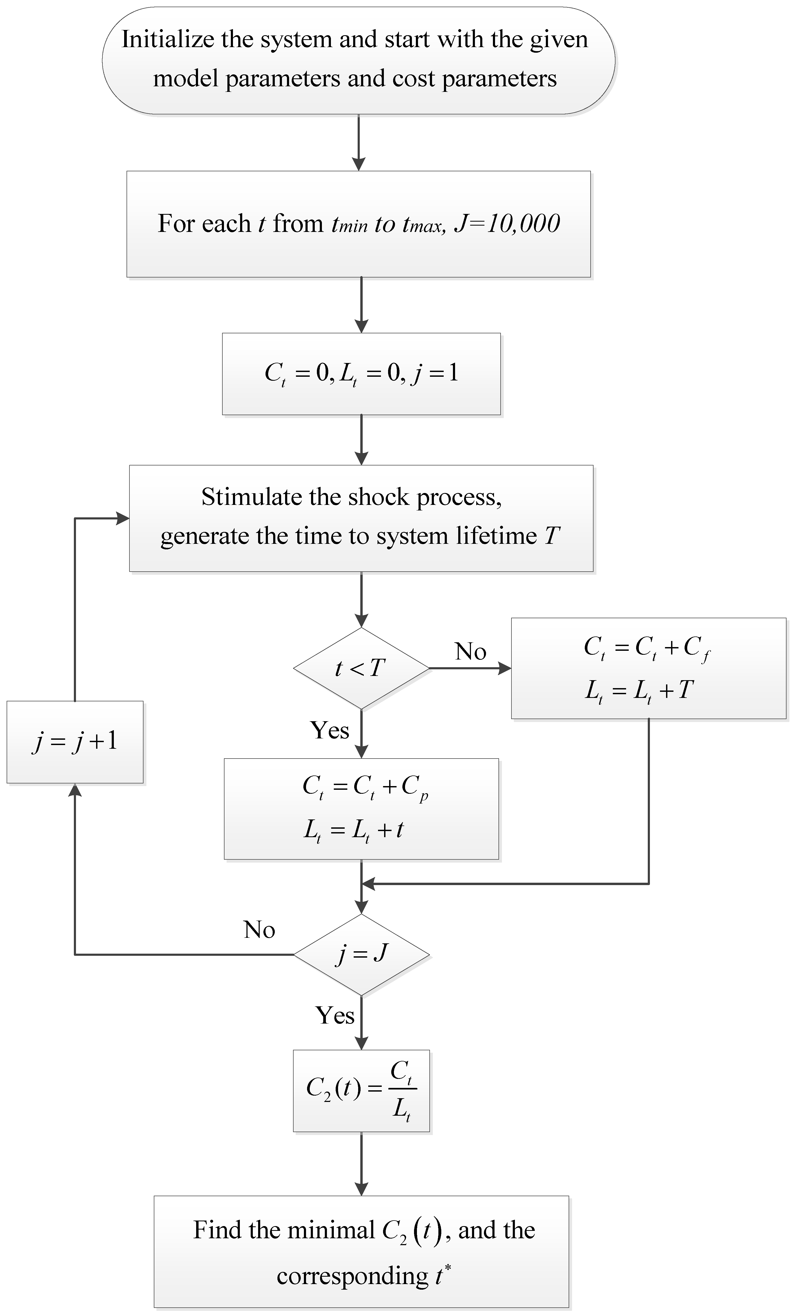
Our aim is to minimize the long-term average cost per unit time, so we need to find the optimal value $t^{\ast }$. By calculating the first derivative of Formula (18), the analytic solution of $t^{\ast }$ can be obtained. In order to verify the results, we employ simulation methods. The flow chart of the algorithm is shown in Figure 3. Let $J$ be the number of simulation runs. Let $C_t$ be the simulated total maintenance cost. Let $L_t$ denote the total cycle length. Then, the average cost per unit time can be obtained as $C_2\left(t\right)=\frac{C_t}{L_t}$. After selecting the appropriate interval $\left(t_{\min },t_{\max }\right)$, we can find the minimum $C_2\left(t\right)$ and the corresponding optimal $t^{\ast }$. Similarly, the preventive maintenance policies under self-exciting trigger mechanism 2 can also be obtained, and the detailed derivation is omitted.

5. Numerical Examples

To validate the proposed model and preventive maintenance strategy, numerical examples are presented in this section. We consider systems running in a random shock environment. The time interval between two adjacent shocks follows exponential distribution. When $n=5$, $k_1=2$, and $m_1=1$, the state space ${\mathsf{\Omega }}_1$ for the Markov chain $\left\{Y_{h_1},h_1\ge 0\right\}$ is constructed as

$${\mathsf{\Omega }}_1=\left\{\left(0,0\right),\left(0,1\right),\left(1,0\right),\left(1,1\right),\left(2,0\right),\left(2,1\right),\left(3,0\right),\left(3,1\right),\left(4,0\right),\left(4,1\right)\right\}\cup \left\{E_a\right\},$$

We obtain the transition probability matrix ${\mathsf{\Lambda }}_1$ as

$$\begin{gathered} {\mathsf{\Lambda }}_1=\begin{array}{c}\left(0,0\right)\\ \left(0,1\right)\\ \left(1,0\right)\\ \left(1,1\right)\\ \left(2,0\right)\\ \left(2,1\right)\\ \left(3,0\right)\\ \left(3,1\right)\\ \left(4,0\right)\\ \left(4,1\right)\\ E_a\end{array}{\left[\begin{array}{ccccccccccc}{q}_2& q_1& p& 0& 0& 0& 0& 0& 0& 0& 0\\ 0& q_2& p+q_1& 0& 0& 0& 0& 0& 0& 0& 0\\ 0& 0& q_2& q_1& p& 0& 0& 0& 0& 0& 0\\ 0& 0& 0& q_2& p+q_1& 0& 0& 0& 0& 0& 0\\ 0& 0& 0& 0& q_2& q_1& p& 0& 0& 0& 0\\ 0& 0& 0& 0& 0& q_2& p+q_1& 0& 0& 0& 0\\ 0& 0& 0& 0& 0& 0& q_2& q_1& p& 0& 0\\ 0& 0& 0& 0& 0& 0& 0& q_2& p+q_1& 0& 0\\ 0& 0& 0& 0& 0& 0& 0& 0& q_2& q_1& p\\ 0& 0& 0& 0& 0& 0& 0& 0& 0& q_2& p+q_1\\ 0& 0& 0& 0& 0& 0& 0& 0& 0& 0& 1\end{array}\right]}_{11\times 11},\mathrm{and}\mathrm{then} \\ {P}_1={\left[\begin{array}{cccccccccc}{q}_2& q_1& p& 0& 0& 0& 0& 0& 0& 0\\ 0& q_2& p+q_1& 0& 0& 0& 0& 0& 0& 0\\ 0& 0& q_2& q_1& p& 0& 0& 0& 0& 0\\ 0& 0& 0& q_2& p+q_1& 0& 0& 0& 0& 0\\ 0& 0& 0& 0& q_2& q_1& p& 0& 0& 0\\ 0& 0& 0& 0& 0& q_2& p+q_1& 0& 0& 0\\ 0& 0& 0& 0& 0& 0& q_2& q_1& p& 0\\ 0& 0& 0& 0& 0& 0& 0& q_2& p+q_1& 0\\ 0& 0& 0& 0& 0& 0& 0& 0& q_2& q_1\\ 0& 0& 0& 0& 0& 0& 0& 0& 0& q_2\end{array}\right]}_{10\times 10},Q_1={\left[\begin{array}{c}0\\ 0\\ 0\\ 0\\ 0\\ 0\\ 0\\ 0\\ p\\ p+q_1\end{array}\right]}_{10\times 1}. \end{gathered}$$

The value of parameters are chosen to be $\lambda =0.55$, $\delta =2$, and $p=0.4$. Then,$q_1=q·P\left\{X_i<\delta \right\}=0.3793$. Then, $q_2=q·P\left\{X_i\ge \delta \right\}=0.2207$. Thus, using Equation (3), we can obtain $E\left(N_1\right)=9.5388$.

When $n=5$, $k_2=2$, and $m_2=1$, the state space ${\mathsf{\Omega }}_2$ for the Markov chain $\left\{Y_{h_2},h_2\ge 0\right\}$ is constructed as

$${\mathsf{\Omega }}_2=\left\{\left(0,0\right),\left(0,1\right),\left(1,0\right),\left(1,1\right),\left(2,0\right),\left(2,1\right),\left(3,0\right),\left(3,1\right),\left(4,0\right),\left(4,1\right)\right\}\cup \left\{E_a\right\}$$

We obtain the transition probability matrix ${\mathsf{\Lambda }}_2$ as

$$\begin{gathered} {\mathsf{\Lambda }}_2=\begin{array}{c}\left(0,0\right)\\ \left(0,1\right)\\ \left(1,0\right)\\ \left(1,1\right)\\ \left(2,0\right)\\ \left(2,1\right)\\ \left(3,0\right)\\ \left(3,1\right)\\ \left(4,0\right)\\ \left(4,1\right)\\ E_a\end{array}{\left[\begin{array}{ccccccccccc}{q}_2& q_1& p& 0& 0& 0& 0& 0& 0& 0& 0\\ q_2& 0& p+q_1& 0& 0& 0& 0& 0& 0& 0& 0\\ 0& 0& q_2& q_1& p& 0& 0& 0& 0& 0& 0\\ 0& 0& q_2& 0& p+q_1& 0& 0& 0& 0& 0& 0\\ 0& 0& 0& 0& q_2& q_1& p& 0& 0& 0& 0\\ 0& 0& 0& 0& q_2& 0& p+q_1& 0& 0& 0& 0\\ 0& 0& 0& 0& 0& 0& q_2& q_1& p& 0& 0\\ 0& 0& 0& 0& 0& 0& q_2& 0& p+q_1& 0& 0\\ 0& 0& 0& 0& 0& 0& 0& 0& q_2& q_1& p\\ 0& 0& 0& 0& 0& 0& 0& 0& q_2& 0& p+q_1\\ 0& 0& 0& 0& 0& 0& 0& 0& 0& 0& 1\end{array}\right]}_{11\times 11},\mathrm{and}\mathrm{then} \\ {P}_2={\left[\begin{array}{cccccccccc}{q}_2& q_1& p& 0& 0& 0& 0& 0& 0& 0\\ q_2& 0& p+q_1& 0& 0& 0& 0& 0& 0& 0\\ 0& 0& q_2& q_1& p& 0& 0& 0& 0& 0\\ 0& 0& q_2& 0& p+q_1& 0& 0& 0& 0& 0\\ 0& 0& 0& 0& q_2& q_1& p& 0& 0& 0\\ 0& 0& 0& 0& q_2& 0& p+q_1& 0& 0& 0\\ 0& 0& 0& 0& 0& 0& q_2& q_1& p& 0\\ 0& 0& 0& 0& 0& 0& q_2& 0& p+q_1& 0\\ 0& 0& 0& 0& 0& 0& 0& 0& q_2& q_1\\ 0& 0& 0& 0& 0& 0& 0& 0& q_2& 0\end{array}\right]}_{10\times 10},Q_2={\left[\begin{array}{c}0\\ 0\\ 0\\ 0\\ 0\\ 0\\ 0\\ 0\\ p\\ p+q_1\end{array}\right]}_{10\times 1}. \end{gathered}$$

The value of parameters are chosen to be $\lambda =0.5$, $\delta =2$, and $p=0.45$, Then $q_1=q·P\left\{X_i<\delta \right\}=0.37$, $q_2=q·P\left\{X_i\ge \delta \right\}=0.22$. Thus, using Equation (9), we can obtain $E\left(N_2\right)=9.9146$.

Reliability Analysis for the Shock Model

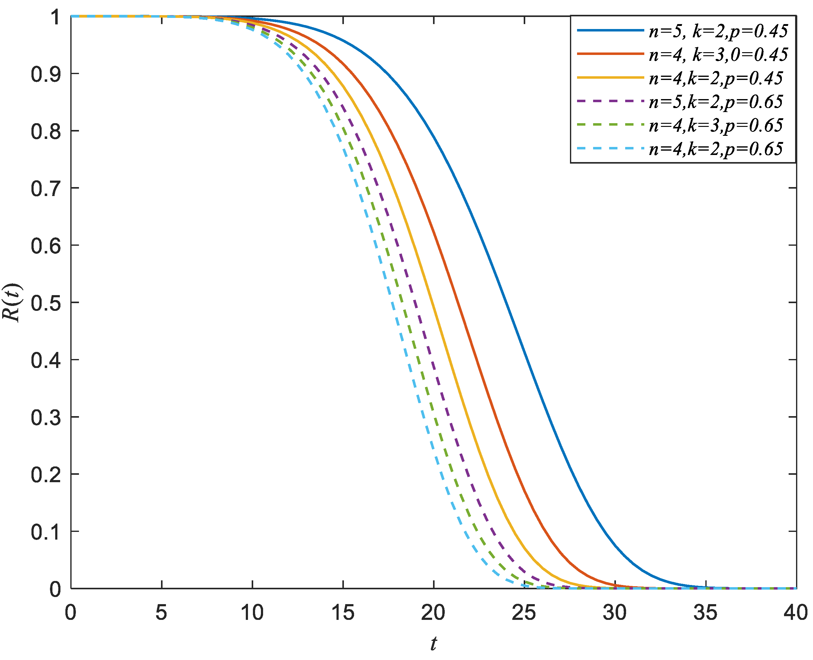
The simulation result of the system reliability under trigger mechanism 1 is presented in Figure 4, where $m_1=1$, $\lambda =0.55$, and $\delta =2$. From Figure 4, we can know that as $n$ increases, the system will fail after more shocks, and the system reliability increases. When $k$ increases, the self-exciting mechanism will be triggered after more shocks, and the reliability of the system increases. When $p$ increases, the probability of the effective shock arrival increases, and the reliability of the system decreases. It can be observed that the system is most reliable when $n=5$, $k_1=2$, and $p=0.45$.

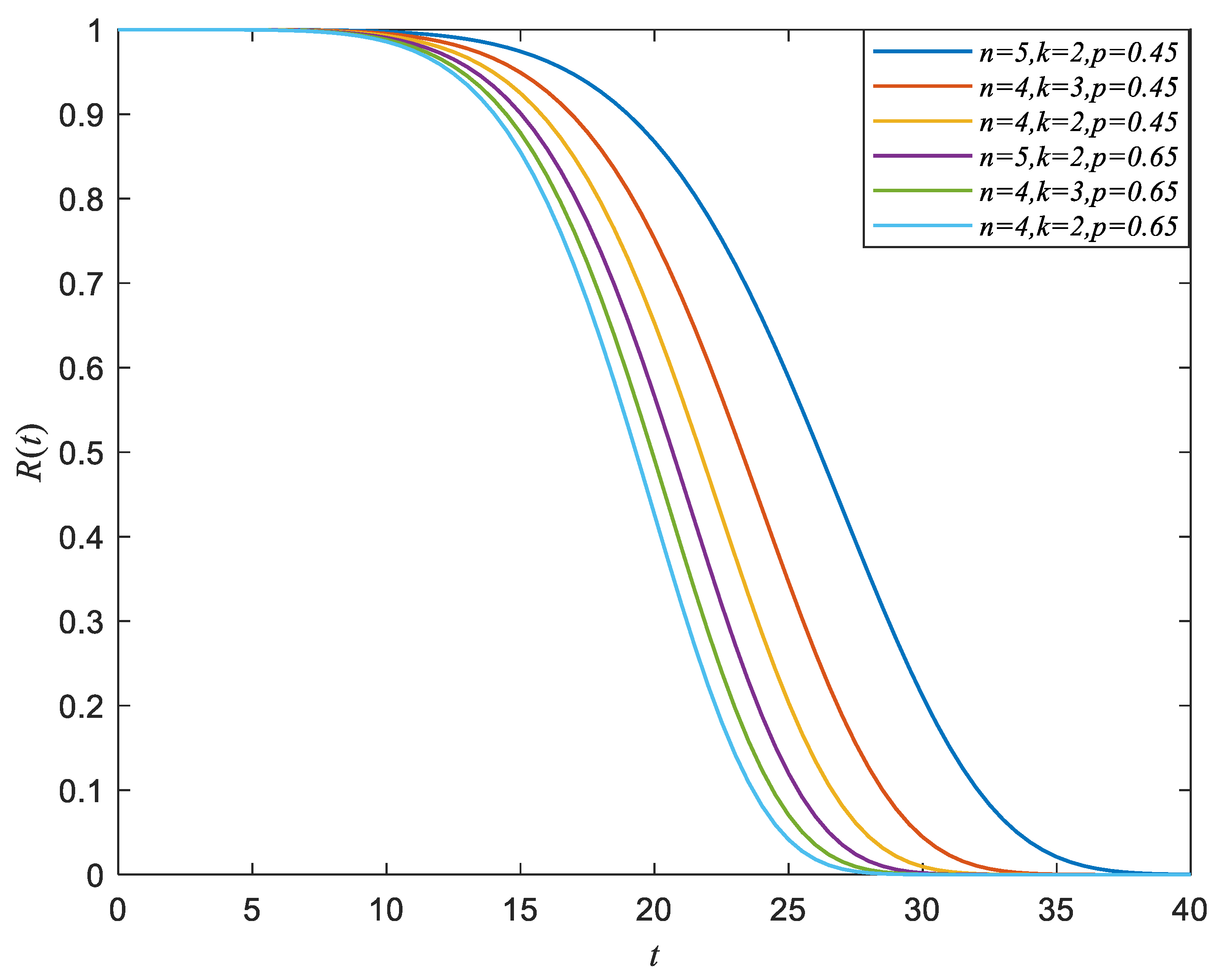
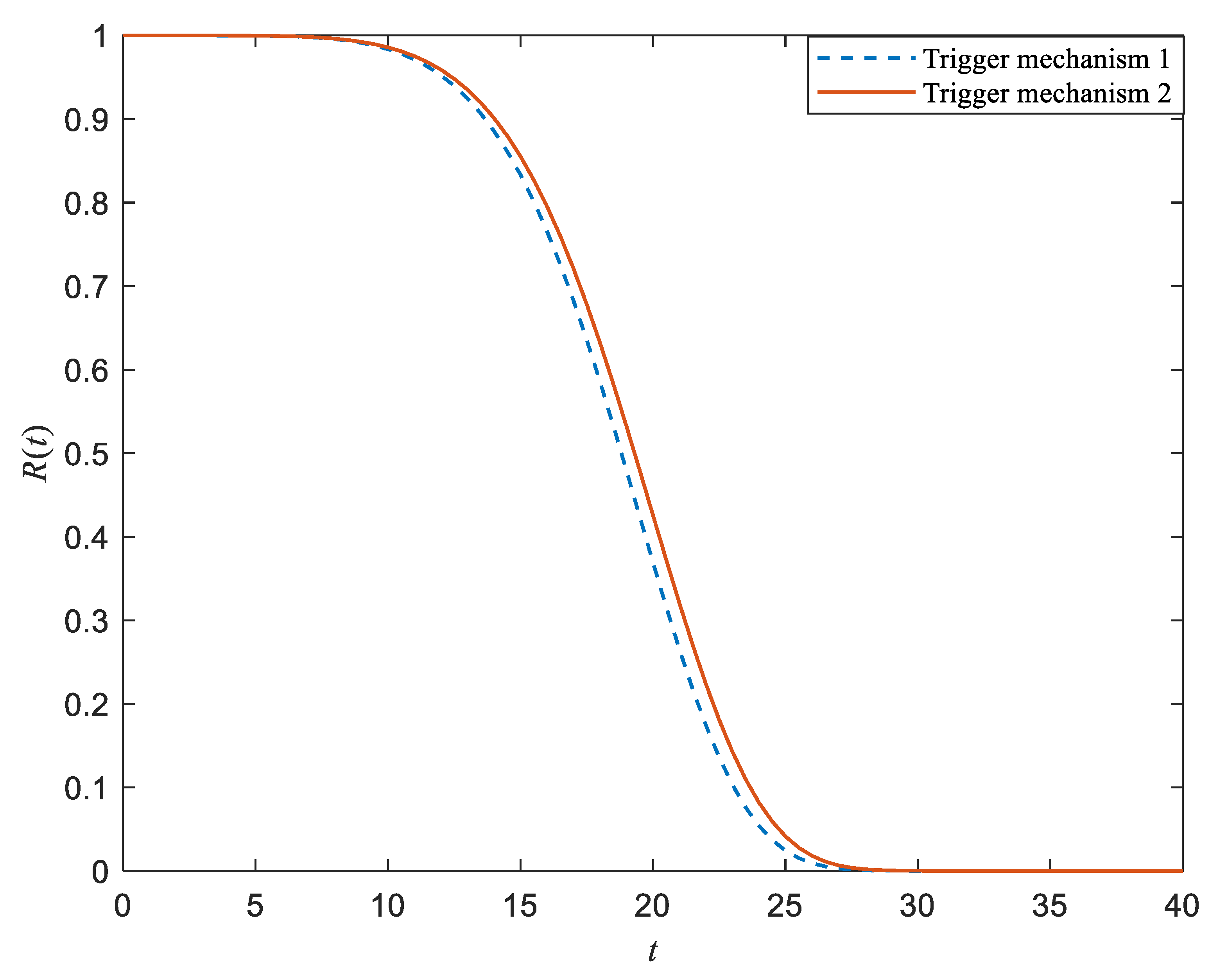
The simulated system reliability under trigger mechanism 2 is presented in Figure 5, where $m_2=1$, $\lambda =0.55$, and $\delta =2$. The effect of $n$, $k_2$ and $p$ on the system reliability is similar to trigger mechanism 1. The reliability of the system is highest when $n=5$, $k_2=2$, and $p=0.4$. The comparison of the simulated system reliability under trigger mechanism 1 and trigger mechanism 2 is presented in Figure 6, where $n=5$, $k=2$, $m=1$, $\lambda =0.55$, $\delta =2$, and $p=0.4$. From Figure 6, we can see that the system reliability under trigger mechanism 2 is higher than the system reliability under trigger mechanism 1.

It can be observed that under self-exciting mechanisms, the reliability is much lower than that under the self-healing mechanism in ref. [23]. Such phenomenon is due to the fact that the damage under a self-exciting mechanism is much larger than that under a self-healing mechanism; thus, the system reliability is lower under self-exciting shock models. Furthermore, the reliability under a self-exciting mechanism is much lower than that under a protective mechanism in a shock environment [37], since the damage is reduced via the protective mechanism, which increases system reliability.

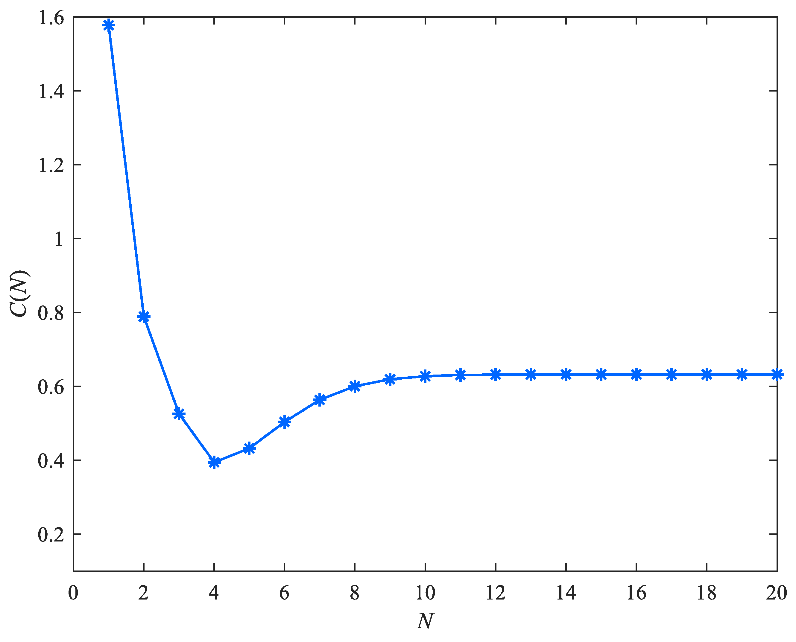
Under maintenance strategy 1, the optimal solution with multiple parameters under trigger mechanism 1 is obtained, as shown in

Table 3. Optimal solution with different parameters when $c_p=2,c_f=5,\lambda =0.55,\delta =2,m_1=1$.

$\mathit{p}$	$\mathit{n}$	$\mathit{k}$	$\mathit{E}\left({\mathit{N}}_1\right)$	${\mathit{N}}^{\ast }$	$\mathit{C}\left({\mathit{N}}^{\ast }\right)$
0.45	3	2	5.7233	4	0.5569
	4	2	7.6310	6	0.4054
	4	3	8470	6	0.3841
	4	4	9.4388	7	0.3783
	5	2	9.5388	7	0.3143
0.75	3	2	4.0910	3	0.6667
	4	2	5.4547	4	0.5
	4	3	5.6590	4	0.5
	4	4	5.7025	4	0.5
	5	2	6.8184	5	0.4

, where we can see that the increase of $p$ leads to the decrease of the optimal value $N^{\ast }$. In other words, the greater the probability of effective shocks arrival, the lower the reliability; thus, the maintenance should be carried out after fewer shocks. $N^{\ast }$ increases with the rise of $n$ or $k$. That is to say, the system can be repaired after more shocks when the system can withstand more shocks before it fails. The system should undergo preventive maintenance after experiencing more shocks if more shocks can trigger the self-exciting mechanism. Figure 7 shows the cost function with several parameters. From Figure 7, we can see that the cost function is convex, and there exists an optimal solution.

The optimal results of different cost parameter values are shown in

Table 4. Optimal solution with different values of cost parameters when $n=5,k=2,p=0.45,\delta =2,m_1=1$.

${\mathit{c}}_{\mathit{p}}$	${\mathit{c}}_{\mathit{f}}$	${\mathit{N}}^{\ast }$	$\mathit{C}\left({\mathit{N}}^{\ast }\right)$
1.5	5.5	6	0.1951
1.5	6.5	6	0.1985
1.5	7.5	6	0.2073
2.5	5.5	7	0.3214
3.5	5.5	8	0.3815

, where $n=5$, $k_1=2$, and $p=0.45$. The results show that the larger $c_p$ is, the larger the optimal solution $N^{\ast }$ is, and the later the replacement time is. When $c_f$ increases, it needs to be replaced in advance.

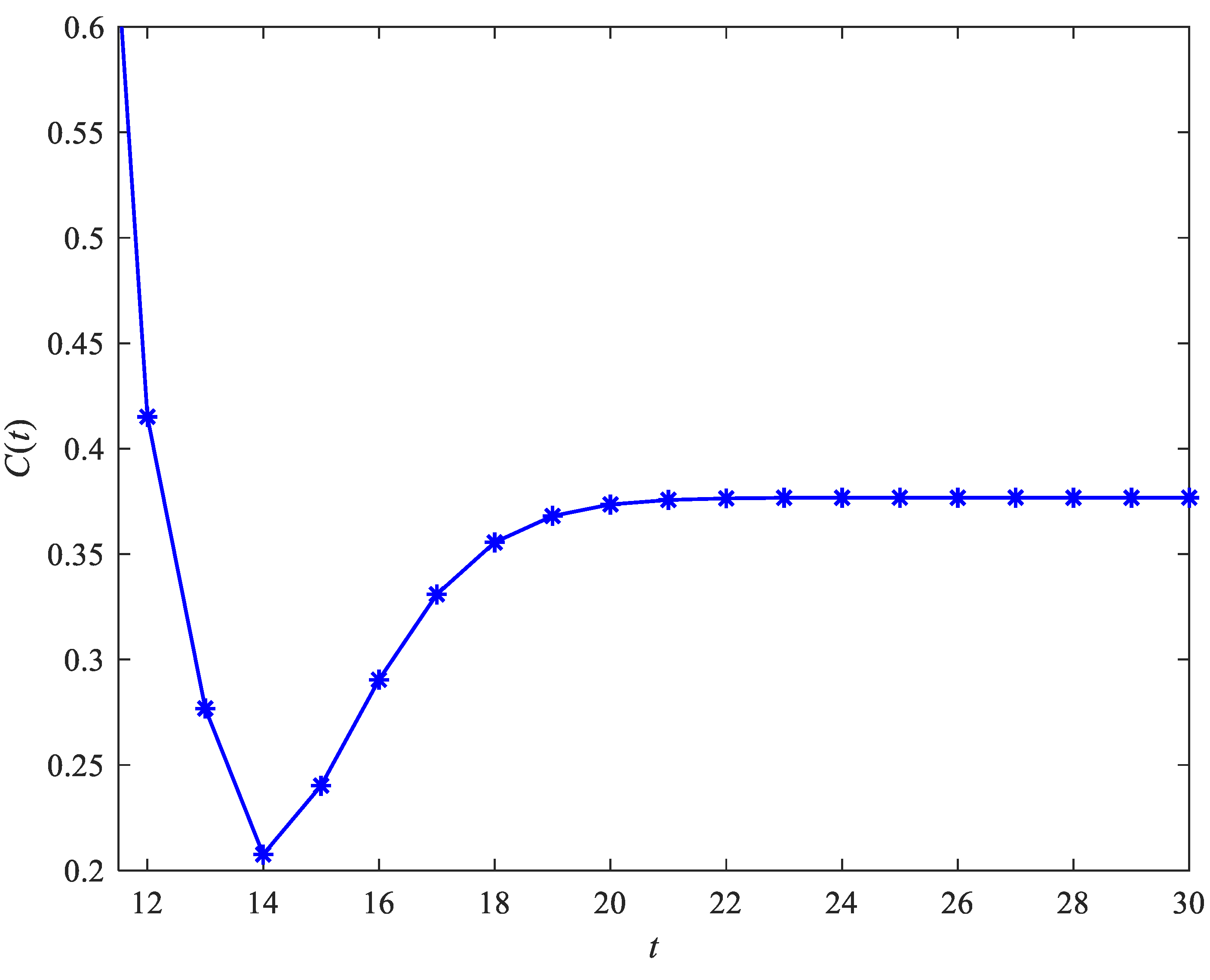
Under maintenance strategy 2, the optimal $t^{\ast }$ and the corresponding $C_2\left(t^{\ast }\right)$ are obtained, as shown in

Table 5. Optimal solution with different parameters when $c_p=2.5,c_f=5.5,\lambda =0.55,\delta =2,m_1=1$.

$\mathit{p}$	$\mathit{n}$	$\mathit{k}$	$\mathit{E}\left(\mathit{T}\right)$	${\mathit{t}}^{\ast }$	${\mathit{C}}_2\left({\mathit{t}}^{\ast }\right)$
0.45	3	2	10.9461	9.8307	0.4510
	4	2	14.8619	11.2785	0.3327
	4	3	17.2837	13.8568	0.2955
	4	4	18.4945	14.7425	0.2836
	5	2	19.5388	13.3568	0.2649
0.75	3	2	7.7819	7.3522	0.6408
	4	2	10.5092	8.2760	0.4615
	4	3	10.8179	8.8378	0.4499
	4	4	11.1049	8.7688	0.4584
	5	2	13.3365	9.4617	0.3631

. As can be observed from Table 5, the increase of $p$ results in the decrease of optimal $t^{\ast }$, implying that the system suffers from more effective shocks, and preventive maintenance should be performed earlier. However, it leads to the increase of the average cost per unit time. The optimal $t^{\ast }$ increases when $n$ increases, which means that the system can withstand more shocks and we can replace the system later. The optimal $t^{\ast }$ increases with the increase of $k$ because a higher $k$ indicates that it is more difficult to trigger the self-exciting mechanism and the system fails later.

Several parameters in the cost function are plotted in Figure 8. Every line in Figure 8 is a convex function, which means that we can find the optimal $t^{\ast }$ to minimize the average cost per unit time. From Figure 8, we can see that the value of $C_2\left(t\right)$ is lowest when $n=5$, $k_1=2$, and $p=0.45$.

The optimal results under different cost parameters are shown in

Table 6. Optimal solution with different values of cost parameters when $n=5,k=2,p=0.45,\delta =2,m_1=1$.

${\mathit{c}}_{\mathit{p}}$	${\mathit{c}}_{\mathit{f}}$	${\mathit{t}}^{\ast }$	${\mathit{C}}_2\left({\mathit{t}}^{\ast }\right)$
1.5	5.5	9.6102	0.1601
1.5	6.5	9.3356	0.1703
1.5	7.5	8.9661	0.1863
2.5	5.5	12.8461	0.2345
3.5	5.5	19.7651	0.2742

, where $n=5$, $k_1=2$, and $p=0.45$. It shows that the larger $c_p$ is, the larger $t^{\ast }$ is, and the later the replacement time is. When $c_f$ increases, it needs to be replaced in advance.

6. Conclusions

This study considers systems subject to random shocks with two types of self-exciting mechanisms and constructs shock models to describe the system failure behavior. On the basis of the proposed shock models, system reliability and expected lifetime are evaluated. According to the shock number and system operation time, two maintenance strategies under different conditions are proposed. Detailed numerical analysis of the reliability models and maintenance strategies are carried out. For further studies, reliability models for systems with multi-components and self-exciting mechanisms could be established. In addition, both internal deterioration and external shock damage with self-exciting mechanisms can be incorporated into the reliability modelling. Finally, other self-exciting mechanisms caused by ineffective shocks can be studied. Future research can take into account the number of ineffective shocks and occurrence time to model self-exciting mechanisms. For example, effective shocks can increase due to the cumulative or consecutive number of shocks in a fixed duration, reaching a threshold.

References

1. Eryilmaz, S. Computing optimal replacement time and mean residual life in reliability shock models. Comput. Ind. Eng. 2016, 103, 40–45. [Google Scholar] [CrossRef]
2. Zhao, X.; Chai, X.; Sun, J.; Qiu, Q. Joint optimization of mission abort and component switching policies for multistate warm standby systems. Reliab. Eng. Syst. Saf. 2021, 212, 107641. [Google Scholar] [CrossRef]
3. Gut, A. Accumulative shock models. Adv. Appl. Probab. 1990, 22, 504–507. [Google Scholar] [CrossRef] [Green Version]
4. Shanthikumar, J.G.; Sumita, U. General Shock Models Associated with Correlated Renewal Sequences. J. Appl. Probab. 1983, 20, 600–614. [Google Scholar] [CrossRef]
5. Mallor, F.; Omey, E. Shocks, runs and random sums. J. Appl. Probab. 2001, 38, 438–448. [Google Scholar] [CrossRef]
6. Li, Z.; Zhao, P. Reliability Analysis on the δ-Shock Model of Complex Systems. IEEE Trans. Reliab. 2007, 56, 340–348. [Google Scholar] [CrossRef]
7. Gut, A.; Hüsler, J. Shock Models. Adv. Degrad. Model. 2010, 7, 541–555. [Google Scholar]
8. Mallor, F.; Omey, E.; Santos, J. Asymptotic results for a run and accumulative mixed shock model. J. Math. Sci. 2006, 138, 5410–5414. [Google Scholar] [CrossRef]
9. Zhao, X.; Li, R.; Fan, Y.; Qiu, Q. Reliability and optimal triggering policy for multi-state systems subject to shocks and supported by a protective device. Comput. Ind. Eng. 2021, 156, 107232. [Google Scholar] [CrossRef]
10. Zhao, X.; Cai, K.; Wang, X.; Song, Y. Optimal replacement policies for a shock model with a change point. Comput. Ind. Eng. 2018, 118, 383–393. [Google Scholar] [CrossRef]
11. Wang, C.; Zhang, H.; Li, Q. Reliability assessment of aging structures subjected to gradual and shock deteriorations. Reliab. Eng. Syst. Saf. 2017, 161, 78–86. [Google Scholar] [CrossRef]
12. Li, X.-Y.; Li, Y.-F.; Huang, H.-Z.; Zio, E. Reliability assessment of phased-mission systems under random shocks. Reliab. Eng. Syst. Saf. 2018, 180, 352–361. [Google Scholar] [CrossRef] [Green Version]
13. Yang, A.; Qiu, Q.; Zhu, M.; Cui, L.; Chen, J. Condition based maintenance strategy for redundant systems with arbitrary structures using improved reinforcement learning. Reliab. Eng. Syst. Saf 2022, 108643. [Google Scholar] [CrossRef]
14. Lin, Y.H.; Li, Y.F.; Zio, E. Reliability assessment of systems subject to dependent degradation processes and random shocks. IIE Trans. 2016, 48, 1072–1085. [Google Scholar] [CrossRef]
15. Zhao, X.; Chai, X.; Sun, J.; Qiu, Q. Optimal bivariate mission abort policy for systems operate in random shock environment. Reliab. Eng. Syst. Saf. 2021, 205, 107244. [Google Scholar] [CrossRef]
16. Qiu, Q.; Cui, L. Reliability evaluation based on a dependent two-stage failure process with competing failures. Appl. Math. Model. 2018, 64, 699–712. [Google Scholar] [CrossRef]
17. Eryilmaz, S.; Kan, C. Reliability and optimal replacement policy for an extreme shock model with a change point. Reliab. Eng. Syst. Saf. 2019, 190, 106513. [Google Scholar] [CrossRef]
18. Qiu, Q.; Cui, L. Optimal mission abort policy for systems subject to random shocks based on virtual age process. Reliab. Eng. Syst. Saf. 2019, 189, 11–20. [Google Scholar] [CrossRef]
19. Eryilmaz, S.; Tekin, M. Reliability evaluation of a system under a mixed shock model. J. Comput. Appl. Math. 2019, 352, 255–261. [Google Scholar] [CrossRef]
20. Chang, C.; Sheu, S.; Chen, Y.; Zhang, Z. A multi-criteria optimal replacement policy for a system subject to shocks. Comput. Ind. Eng. 2011, 61, 1035–1043. [Google Scholar] [CrossRef]
21. Qiu, Q.; Cui, L.; Dong, Q. Preventive maintenance policy of single-unit systems based on shot-noise process. Qual. Reliab. Eng. Int. 2019, 35, 550–560. [Google Scholar] [CrossRef]
22. Toshio, N. Further Results of Replacement Problem of a Parallel System in Random Environment. J. Appl. Probab. 1979, 16, 923–926. [Google Scholar] [CrossRef]
23. Zhao, X.; Guo, X.; Wang, X. Reliability and maintenance policies for a two-stage shock model with self-healing mechanism. Reliab. Eng. Syst. Saf. 2018, 172, 185–194. [Google Scholar] [CrossRef]
24. Zhao, X.; Lv, Z.; He, Z.; Wang, W. Reliability and opportunistic maintenance for a series system with multi-stage accelerated damage in shock environments. Comput. Ind. Eng. 2019, 137, 106029. [Google Scholar] [CrossRef]
25. Wang, Q.; He, Z.; Lin, S.; Li, Z. Failure Modeling and Maintenance Decision for GIS Equipment Subject to Degradation and Shocks. IEEE Trans. Power Deliv. 2017, 32, 1079–1088. [Google Scholar] [CrossRef]
26. Yang, L.; Ma, X.; Zhao, Y. A condition-based maintenance model for a three-state system subject to degradation and environmental shocks. Comput. Ind. Eng. 2017, 105, 210–222. [Google Scholar] [CrossRef]
27. Wang, J.; Qiu, Q.; Wang, H.; Lin, C. Optimal condition-based preventive maintenance policy for balanced systems. Reliab. Eng. Syst. Saf. 2021, 211, 107606. [Google Scholar] [CrossRef]
28. Zhao, X.; Chai, X.; Sun, J.; Qiu, Q. Joint optimization of mission abort and protective device selection policies for multistate systems. Risk Anal. 2022. [Google Scholar] [CrossRef]
29. Qiu, Q.; Cui, L. Reliability modelling based on dependent two-stage virtual age processes. J. Syst. Eng. Electron. 2021, 32, 711–721. [Google Scholar]
30. Wang, J.; Qiu, Q.; Wang, H. Joint optimization of condition-based and age-based replacement policy and inventory policy for a two-unit series system. Reliab. Eng. Syst. Saf. 2021, 205, 107251. [Google Scholar] [CrossRef]
31. Liu, H.; Yeh, R.H.; Cai., B. Reliability modeling for dependent competing failure processes of damage self-healing systems. Comput. Ind. Eng 2017, 105, 55–62. [Google Scholar] [CrossRef]
32. Cha, J.H.; Finkelstein, M. A note on ‘curable’ shock processes. J. Stat. Plan. Inference 2012, 142, 3146–3151. [Google Scholar] [CrossRef]
33. Cui, L.; Chen, Z.; Gao, H. Reliability for systems with self-healing effect under shock models. Nephron Clin. Pract. 2018, 15, 551–567. [Google Scholar] [CrossRef]
34. Borovykh, A.; Pascucci, A.; Rovere, S.L. Systemic risk in a mean-field model of interbank lending with self-exciting shocks. IISE Trans. 2018, 50, 806–819. [Google Scholar] [CrossRef]
35. Chen, Y.; Singpurwalla, N.D. Unification of Software Reliability Models by Self-Exciting Point Processes. Adv. Appl. Probab. 1997, 29, 337–352. [Google Scholar] [CrossRef]
36. Wang, R. A mixture and self-exciting model for software reliability. Stats Probab. Lett. 2005, 72, 187–194. [Google Scholar] [CrossRef]
37. Wu, Y.; Qiu, Q. Optimal Triggering Policy of Protective Devices Considering Self-Exciting Mechanism of Shocks. Mathematics 2022, 10, 2732. [Google Scholar] [CrossRef]
Figure 1. Failure process of the system under self-exciting trigger mechanism 1. (a denotes the type of shock and b denotes the shock occurrence time).
Applsci 12 10418 g001
Figure 2. Failure process of the system under self-exciting trigger mechanism 2. (a denotes the type of shock and b denotes the shock occurrence time).
Applsci 12 10418 g002
Figure 3. Simulation flowchart under maintenance policy 2.
Applsci 12 10418 g003
Figure 4. Simulation result of the system reliability under trigger mechanism 1.
Applsci 12 10418 g004
Figure 5. Simulation result of the system reliability under trigger mechanism 2.
Applsci 12 10418 g005
Figure 6. The comparison of different trigger mechanisms.
Applsci 12 10418 g006
Figure 7. Cost under maintenance policy 1.
Applsci 12 10418 g007
Figure 8. Cost function under different parameters.
Applsci 12 10418 g008