
Contour Propagation for Radiotherapy Treatment Planning Using Nonrigid Registration and Parameter Optimization: Case Studies in Liver and Breast Cancer

 , and
, and
Abstract
1. Introduction
2. Methodology
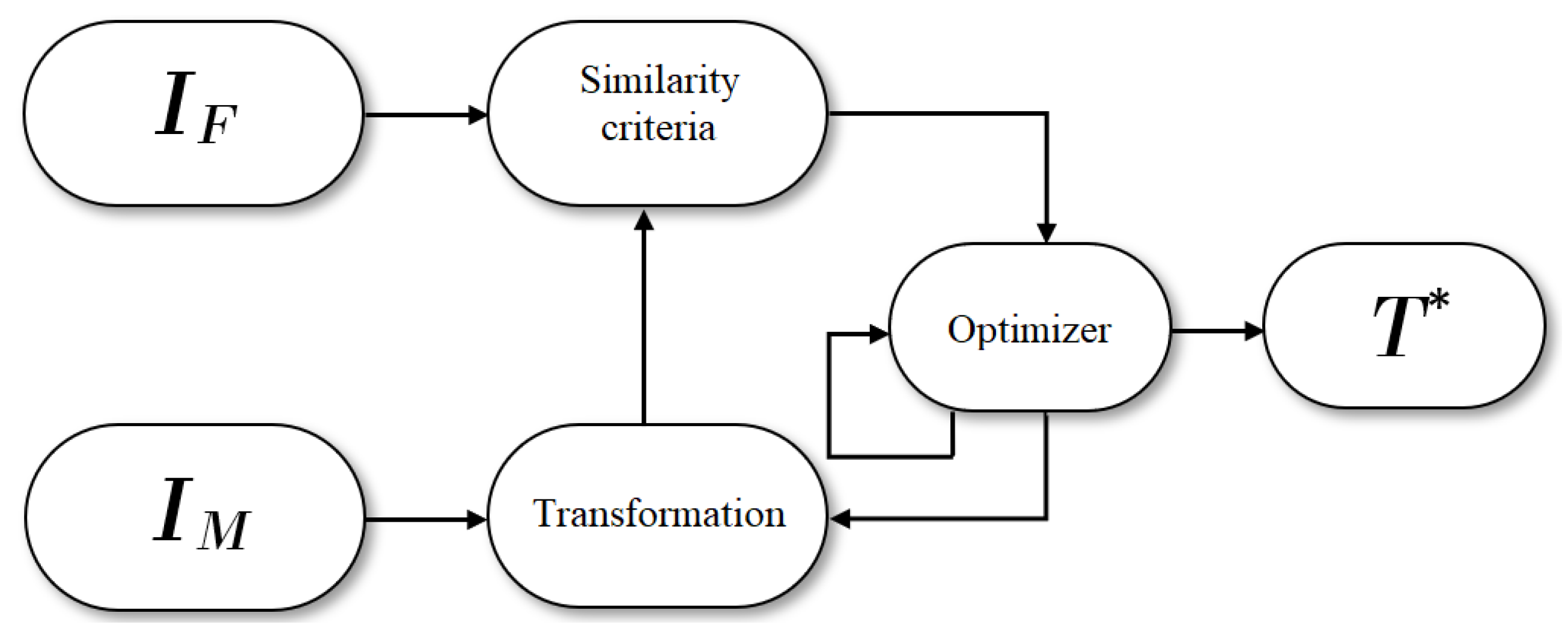
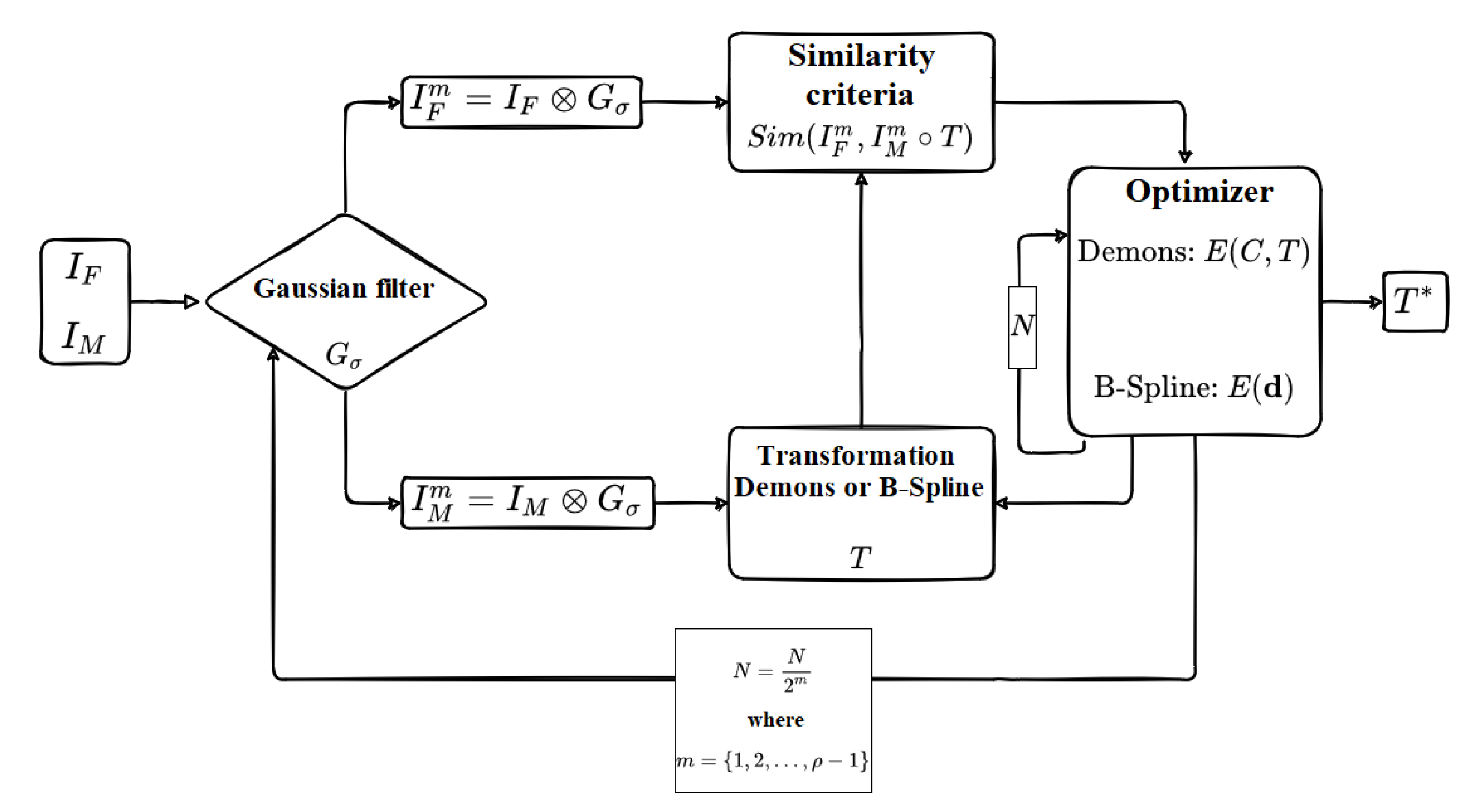
2.1. Image Registration
2.2. Demon Algorithm
2.3. Algorithm Based on B-Spline
2.4. Performance Measures
2.4.1. Dice Coefficient
2.4.2. Correlation Coefficient (CC)
2.5. Data Structure and Preprocessing
Breast CT Acquisition in 4-D Format
3. Results and Discussion of Computational Experiments
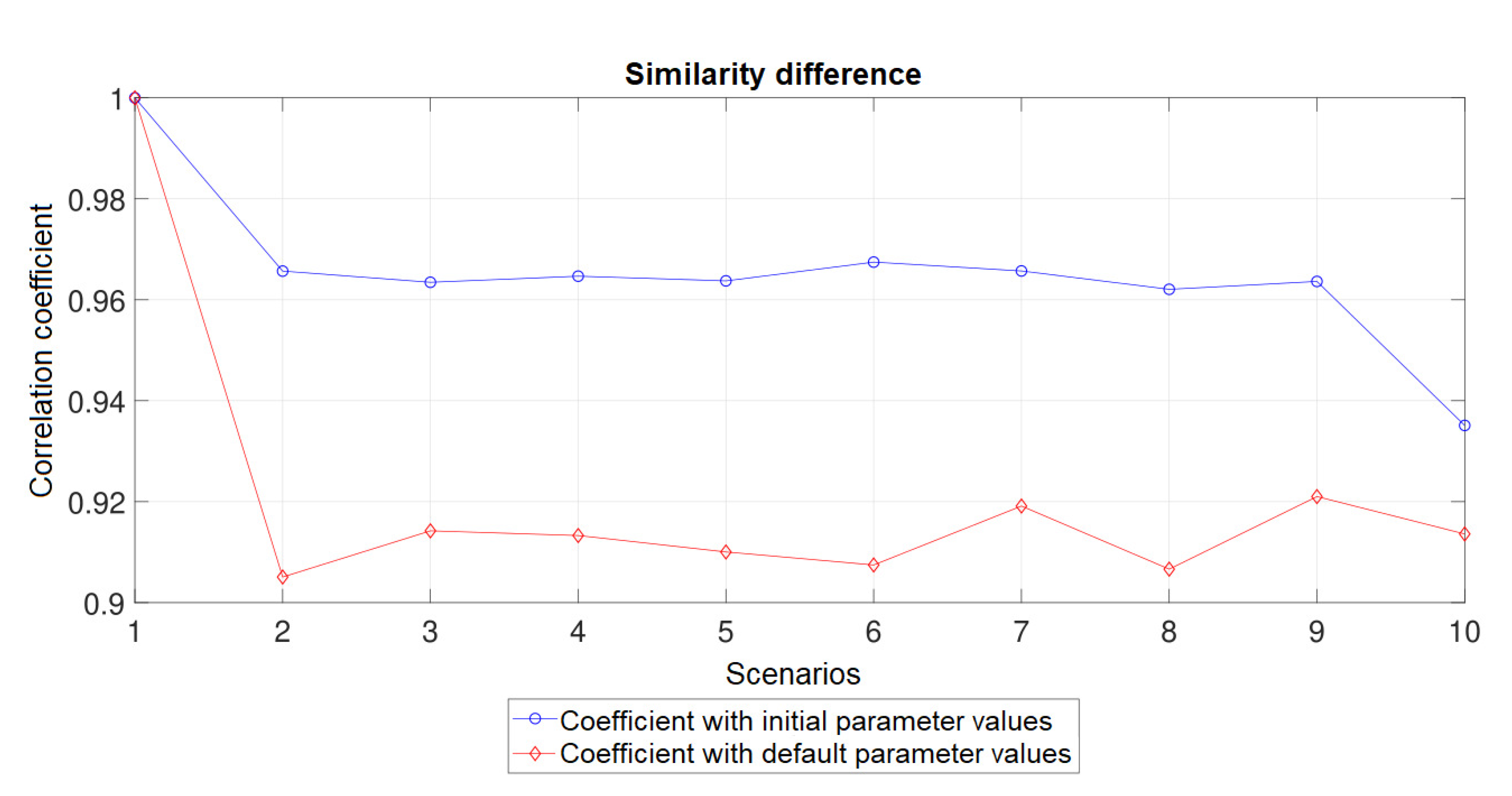
3.1. Parametrization of the Demons Algorithm
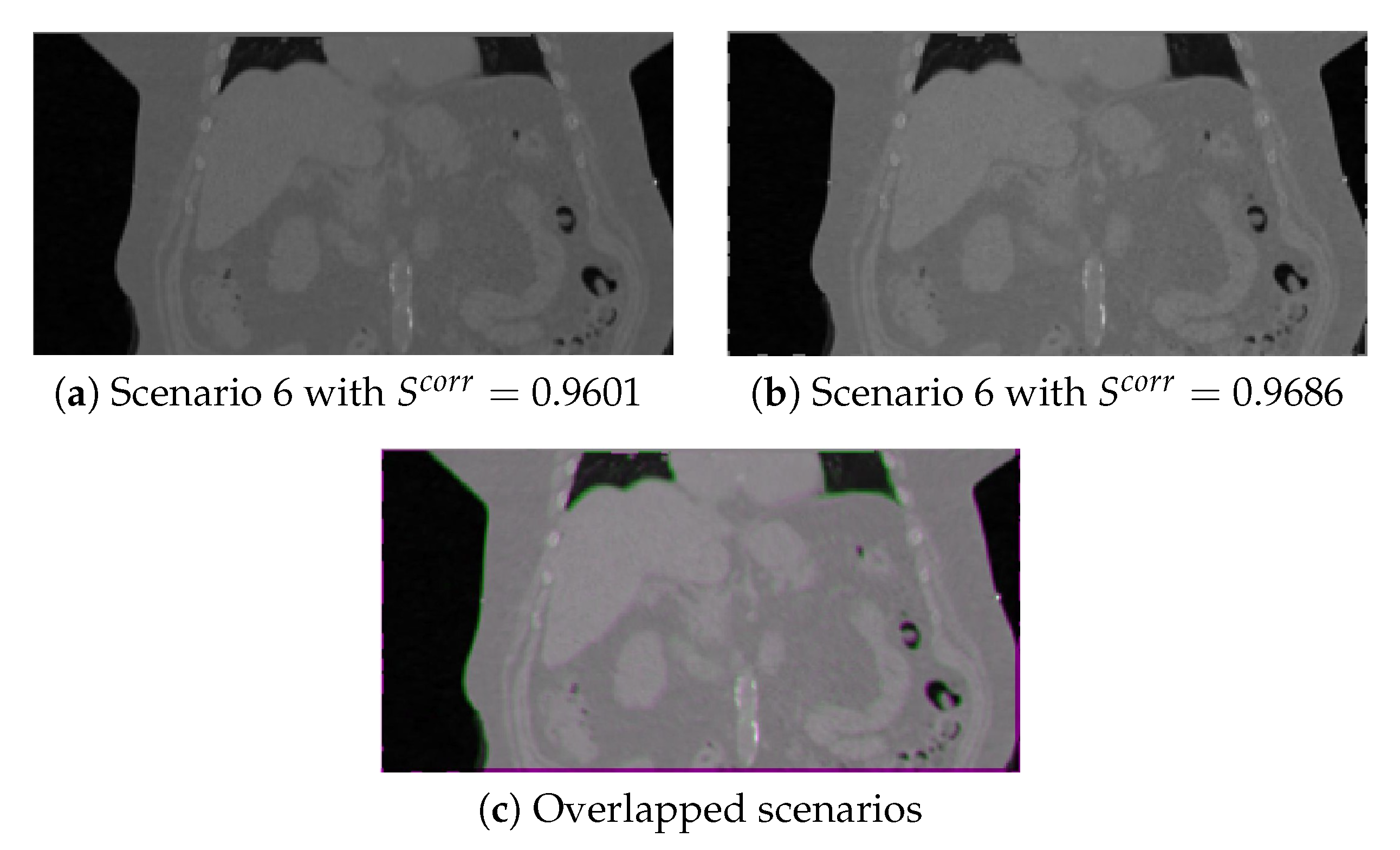
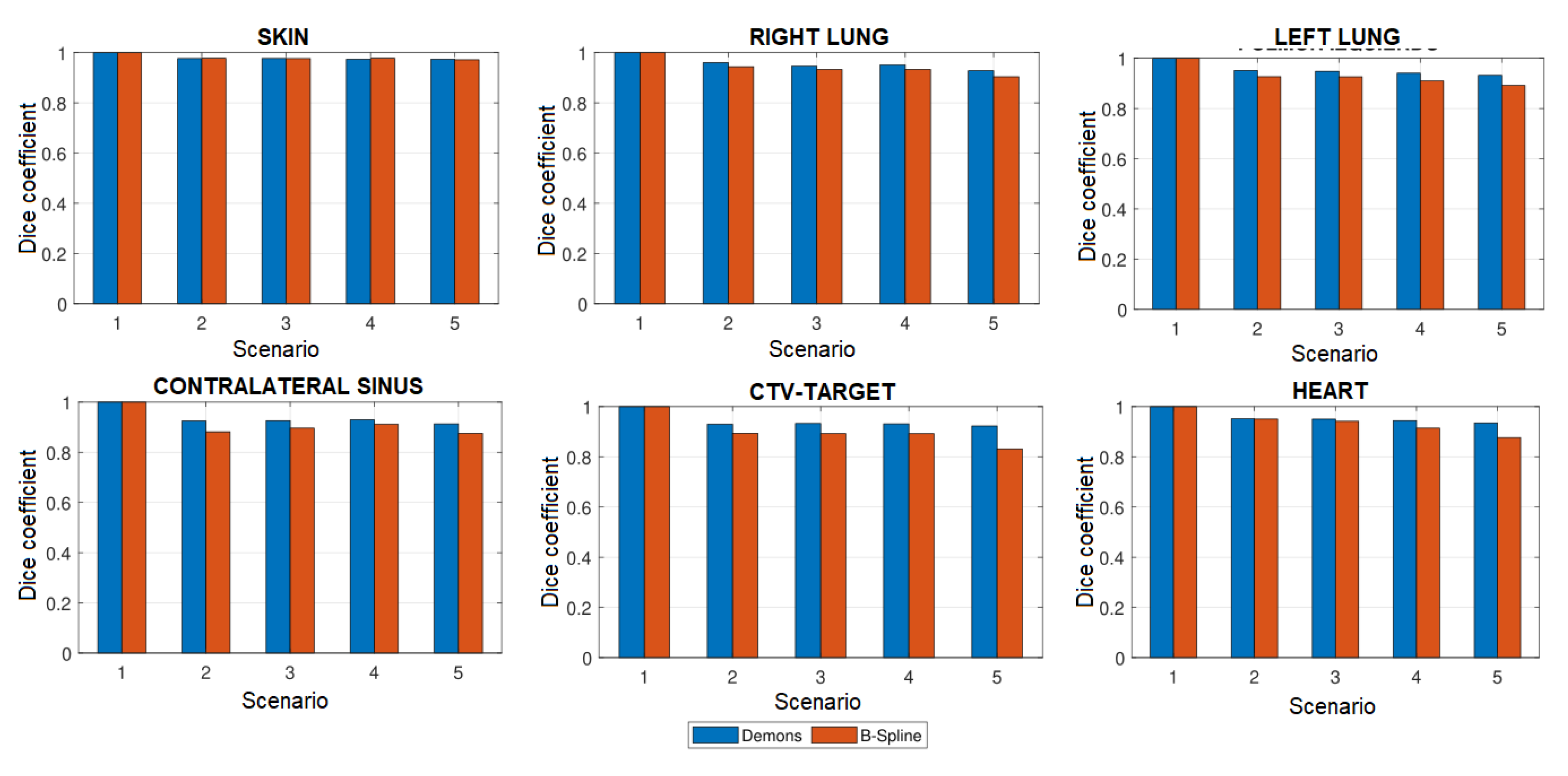
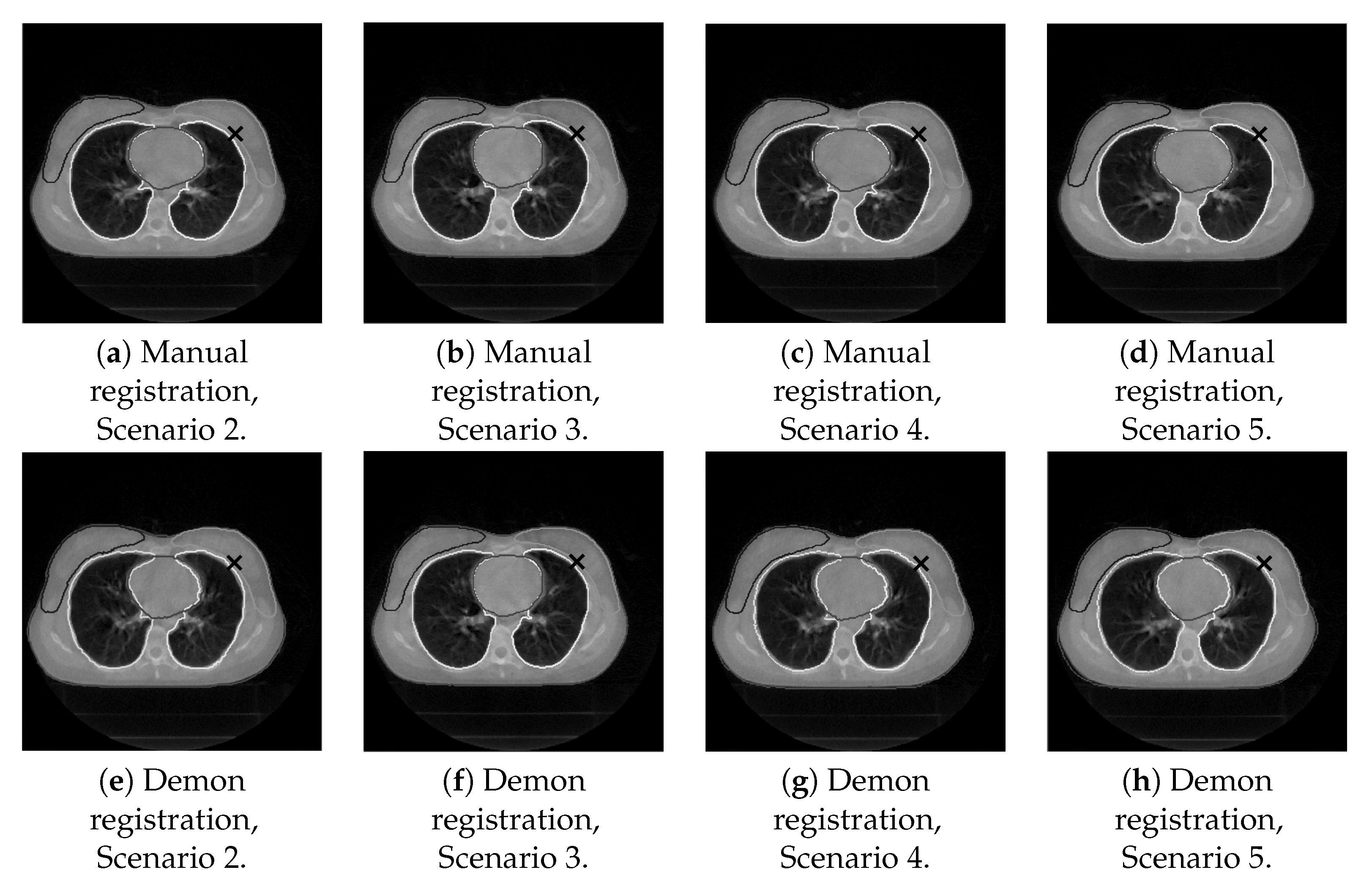
3.2. Contour-Propagation Algorithm
| Algorithm 1: matRad-contourPropagation |
Input: CT scans for the n scenarios and SCT for the fixed scenario. Output: CT scans for the n scenarios and SCT for the m structures. for scenario do Calculate DVF end for for structure do Convert linear indices of SCT structure j for Scenario 1 into a cube () for scenario do Apply to the structure j for scenario 1 to estimate structure j for scenario i Convert the cube of structure j for Scenario i into linear indices Store the structure j in the SCT for Scenario i end for end for |
4. Conclusions
Author Contributions
Funding
Institutional Review Board Statement
Informed Consent Statement
Data Availability Statement
Acknowledgments
Conflicts of Interest
Abbreviations
| CC | Correlation coefficient |
| CT | Computerized tomography |
| CTV | Clinical treatment volume |
| DCS | Dice similarity coefficient |
| DVF | Displacement vector field |
| FFD | Free form deformation |
| MRI | Magnetic resonance imaging |
| MSE | Mean squared error |
| OF | Optical flow |
| SCT | Segmented computed tomography |
| VOI | Volume of interest |
References
- Bookstein, F.L. Principal warps: Thin-plate splines and the decomposition of deformations. IEEE Trans. Pattern Anal. Mach. Intell. 1989, 11, 567–585. [Google Scholar] [CrossRef]
- Kumar, R.; Asmuth, J.C.; Hanna, K.; Bergen, J.R.; Hulka, C.; Kopans, D.B.; Weisskoff, R.; Moore, R.H. Application of 3D registration for detecting lesions in magnetic resonance breast scans. In Medical Imaging 1996: Image Processing; International Society for Optics and Photonics, SPIE: Newport Beach, CA, USA, 1996; Volume 2710, pp. 646–656. [Google Scholar] [CrossRef]
- Rueckert, D.; Sonoda, L.I.; Hayes, C.; Hill, D.L.G.; Leach, M.O.; Hawkes, D.J. Nonrigid registration using free-form deformations: Application to breast MR images. IEEE Trans. Med. Imaging. 1999, 18, 712–721. [Google Scholar] [CrossRef] [PubMed]
- Mattes, D.; Haynor, D.R.; Vesselle, H.; Lewellen, T.K.; Eubank, W. PET-CT image registration in the chest using free-form deformations. IEEE Trans. Med. Imaging 2003, 22, 120–128. [Google Scholar] [CrossRef] [PubMed]
- Du, S.; Liu, J.; Zhang, C.; Xu, M.; Xue, J. Accurate non-rigid registration based on heuristic tree for registering point sets with large deformation. Neurocomputing 2015, 168, 681–689. [Google Scholar] [CrossRef]
- Mai Elfarnawany, S.; Alam, R.; Agrawal, S.K.; Ladak, H.M. Evaluation of non-rigid registration parameters for atlas-based segmentation of CT images of human cochlea. In Medical Imaging 2017: Image Processing; Styner, M.A., Angelini, E.D., Eds.; International Society for Optics and Photonics, SPIE: Newport Beach, CA, USA, 2017; Volume 10133, pp. 283–289. [Google Scholar] [CrossRef]
- Santos, J.; Chaudhari, A.J.; Joshi, A.A.; Ferrero, A.; Yang, K.; Boone, J.M.; Badawi, R.D. Non-rigid registration of serial dedicated breast CT, longitudinal dedicated breast CT and PET/CT images using the diffeomorphic demons method. Phys. Medica 2014, 30, 713–717. [Google Scholar] [CrossRef] [PubMed][Green Version]
- Mesbah, M. Gradient-based optical flow: A critical review. In Proceedings of the 5th International Symposium on Signal Processing and Its Applications, Brisbane, Australia, 22–25 August 1999; Volume 1, pp. 467–470. [Google Scholar] [CrossRef]
- Chakraborty, S.; Dey, N.; Samanta, S.; Ashour, A.S.; Barna, C.; Balas, M.M. Optimization of Non-rigid Demons Registration Using Cuckoo Search Algorithm. Cogn. Comput. 2017, 9, 817–826. [Google Scholar] [CrossRef]
- Folgoc, L.L.; Delingette, H.; Criminisi, A.; Ayache, N. Sparse Bayesian registration of medical images for self-tuning of parameters and spatially adaptive parametrization of displacements. Med. Image Anal. 2017, 36, 79–97. [Google Scholar] [CrossRef] [PubMed]
- Wang, M.; Li, P. A Review of Deformation Models in Medical Image Registration. J. Med. Biol. Eng. 2019, 39, 1–17. [Google Scholar] [CrossRef]
- Thirion, J.P. Image matching as a diffusion process: An analogy with Maxwell’s demons. Med. Image Anal. 1998, 2, 243–260. [Google Scholar] [CrossRef]
- Horn, B.K.; Schunck, B.G. Determining Optical Flow. In Techniques and Applications of Image Understanding; Pearson, J.J., Ed.; International Society for Optics and Photonics, SPIE: Washington, DC, USA, 1981; Volume 0281, pp. 319–331. [Google Scholar] [CrossRef]
- Vercauteren, T.; Pennec, X.; Malis, E.; Perchant, A.; Ayache, N. Insight into Efficient Image Registration Techniques and the Demons Algorithm. In Information Processing in Medical Imaging; Karssemeijer, N., Lelieveldt, B., Eds.; Springer: Berlin/Heidelberg, Germany, 2007; pp. 495–506. [Google Scholar]
- Hernandez, M.; Bossa, M.N.; Olmos, S. Registration of anatomical images using geodesic paths of diffeomorphisms parameterized with stationary vector fields. In Proceedings of the 2007 IEEE 11th International Conference on Computer Vision, Rio De Janeiro, Brazil, 14–21 October 2007; pp. 1–8. [Google Scholar] [CrossRef]
- Ashburner, J. A fast diffeomorphic image registration algorithm. NeuroImage 2007, 38, 95–113. [Google Scholar] [CrossRef]
- Vercauteren, T.; Pennec, X.; Perchant, A.; Ayache, N. Diffeomorphic demons: Efficient non-parametric image registration. NeuroImage 2009, 45, S61–S72. [Google Scholar] [CrossRef]
- Jähne, B. Displacement Vector Fields. In Digital Image Processing: Concepts, Algorithms, and Scientific Applications; Springer: Berlin/Heidelberg, Germany, 1993; pp. 297–317. [Google Scholar] [CrossRef]
- Barron, J.L.; Fleet, D.J.; Beauchemin, S.S. Performance of optical flow techniques. Int. J. Comput. Vis. 1994, 12, 43–77. [Google Scholar] [CrossRef]
- Hermosillo, G.; Chefd’Hotel, C.; Faugeras, O. Variational Methods for Multimodal Image Matching. Int. J. Comput. Vis. 2002, 50, 329–343. [Google Scholar] [CrossRef]
- Cachier, P.; Bardinet, E.; Dormont, D.; Pennec, X.; Ayache, N. Iconic feature based nonrigid registration: The PASHA algorithm. Comput. Vis. Image Underst. 2003, 89, 272–298. [Google Scholar] [CrossRef]
- Benhimane, S.; Malis, E. Real-time image-based tracking of planes using efficient second-order minimization. In Proceedings of the 2004 IEEE/RSJ International Conference on Intelligent Robots and Systems (IROS), Sendai, Japan, 28 September–2 October 2004; Volume 1, pp. 943–948. [Google Scholar] [CrossRef]
- Mahony, R.; Manton, J.H. The Geometry of the Newton Method on Non-Compact Lie Groups. J. Glob. Optim. 2002, 23, 309–327. [Google Scholar] [CrossRef]
- Bardinet, E.; Cohen, L.D.; Ayache, N. Tracking and motion analysis of the left ventricle with deformable superquadrics. Med. Image Anal. 1996, 1, 129–149. [Google Scholar] [CrossRef]
- Lee, S.; Wolberg, G.; Shin, S.Y. Scattered data interpolation with multilevel B-splines. IEEE Trans. Vis. Comput. Graph. 1997, 3, 228–244. [Google Scholar] [CrossRef]
- Lee, S.; Wolberg, G.; Chwa, K.; Shin, S.Y. Image metamorphosis with scattered feature constraints. IEEE Trans. Vis. Comput. Graph. 1996, 2, 337–354. [Google Scholar] [CrossRef]
- Vishnevskiy, V.; Gass, T.; Szekely, G.; Tanner, C.; Goksel, O. Isotropic Total Variation Regularization of Displacements in Parametric Image Registration. IEEE Trans. Med. Imaging 2017, 36, 385–395. [Google Scholar] [CrossRef] [PubMed]
- Wieser, H.P.; Cisternas, E.; Wahl, N.; Ulrich, S.; Stadler, A.; Mescher, H.; Müller, L.R.; Klinge, T.; Gabrys, H.; Burigo, L.; et al. Development of the open-source dose calculation and optimization toolkit matRad. Med. Phys. 2017, 44, 2556–2568. [Google Scholar] [CrossRef] [PubMed]
- Cahill, N.D.; Noble, J.A.; Hawkes, D.J. A Demons Algorithm for Image Registration with Locally Adaptive Regularization. In Medical Image Computing and Computer-Assisted Intervention—MICCAI 2009; Yang, G.Z., David, H., Daniel Rueckert, A.N., Taylor, C., Eds.; Springer: Berlin/Heidelberg, Germany, 2009; pp. 574–581. [Google Scholar]


| Scenario | Initial Parameters | Local Optima |
|---|---|---|
| Parameters | ||
| , , 2.5 | , , 2.9 | |
| 1 | 1.0000 | 1.0000 |
| 2 | 0.9562 | 0.9585 |
| 3 | 0.9538 | 0.9611 |
| 4 | 0.9540 | 0.9608 |
| 5 | 0.9495 | 0.9580 |
| 6 | 0.9430 | 0.9582 |
| 7 | 0.9629 | 0.9641 |
| 8 | 0.9575 | 0.9635 |
| 9 | 0.9619 | 0.9640 |
| 10 | 0.9576 | 0.9629 |
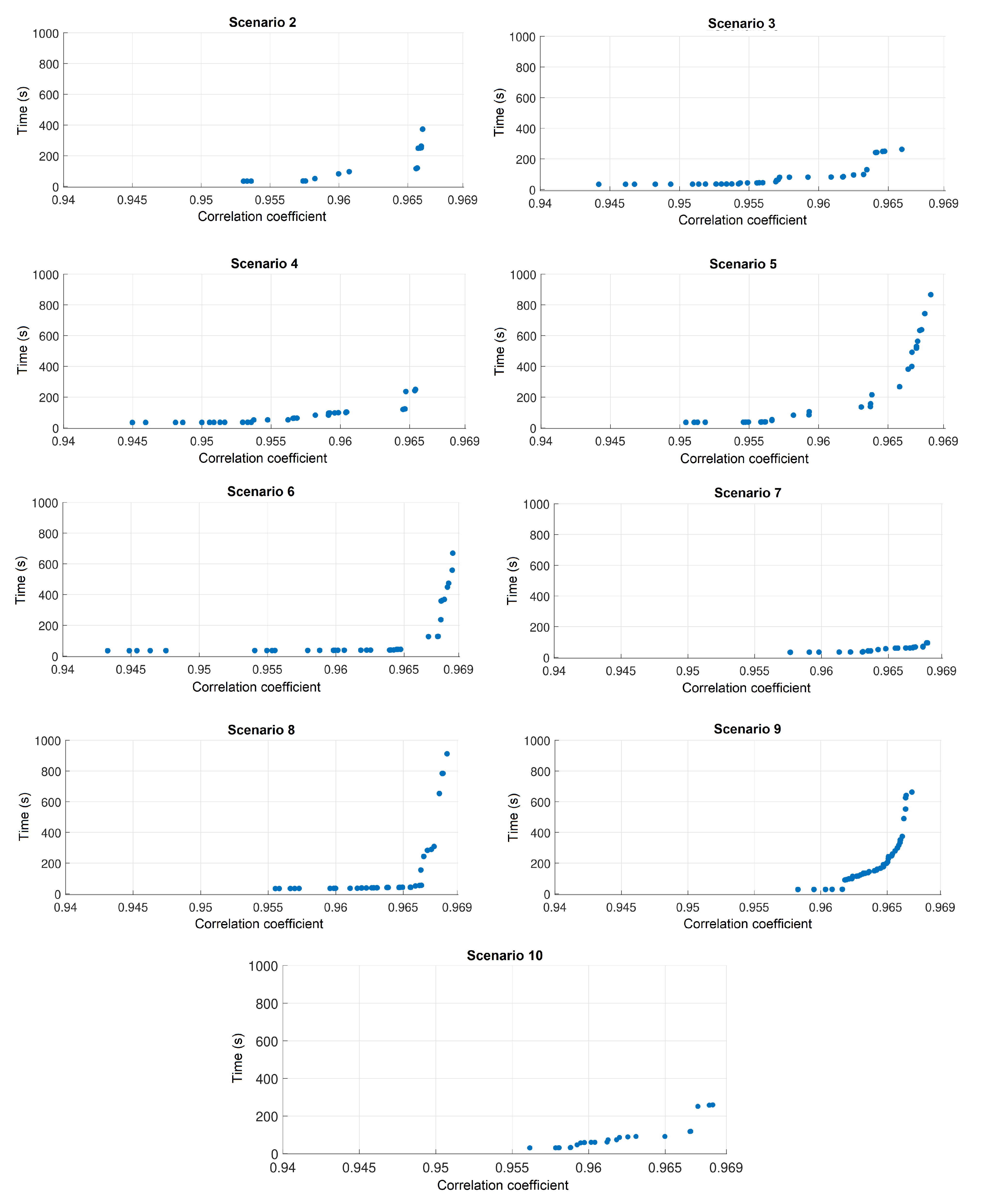
| Scenario | Time Increment | Correlation Coefficient | Correlation Coefficient |
|---|---|---|---|
| Ratio | Interval Length | Center Value | |
| 2 | 3.5455 | 0.0061 | 0.9658 |
| 3 | 2.2114 | 0.0051 | 0.9635 |
| 4 | 1.5268 | 0.0050 | 0.9646 |
| 5 | 5.4101 | 0.0050 | 0.9667 |
| 6 | 16.7341 | 0.0084 | 0.9657 |
| 7 | 1.7081 | 0.0066 | 0.9657 |
| 8 | 24.2389 | 0.0083 | 0.9648 |
| 9 | 21.8860 | 0.0065 | 0.9645 |
| 10 | 3.3256 | 0.0079 | 0.9626 |
| Scenario 1 | Scenario 2 | Scenario 3 | Scenario 4 | Scenario 5 | |
|---|---|---|---|---|---|
| 1 | 1 | 1 | 1 | 1 | |
| N | 100 | 100 | 100 | 100 | 100 |
| 1.5 | 1.5 | 2.6 | 1.8 | 2.9 |
Publisher’s Note: MDPI stays neutral with regard to jurisdictional claims in published maps and institutional affiliations. |
© 2022 by the authors. Licensee MDPI, Basel, Switzerland. This article is an open access article distributed under the terms and conditions of the Creative Commons Attribution (CC BY) license (https://creativecommons.org/licenses/by/4.0/).
Share and Cite
Vargas-Bedoya, E.; Rivera, J.C.; Puerta, M.E.; Angulo, A.; Wahl, N.; Cabal, G. Contour Propagation for Radiotherapy Treatment Planning Using Nonrigid Registration and Parameter Optimization: Case Studies in Liver and Breast Cancer. Appl. Sci. 2022, 12, 8523. https://doi.org/10.3390/app12178523
Vargas-Bedoya E, Rivera JC, Puerta ME, Angulo A, Wahl N, Cabal G. Contour Propagation for Radiotherapy Treatment Planning Using Nonrigid Registration and Parameter Optimization: Case Studies in Liver and Breast Cancer. Applied Sciences. 2022; 12(17):8523. https://doi.org/10.3390/app12178523
Chicago/Turabian StyleVargas-Bedoya, Eliseo, Juan Carlos Rivera, Maria Eugenia Puerta, Aurelio Angulo, Niklas Wahl, and Gonzalo Cabal. 2022. "Contour Propagation for Radiotherapy Treatment Planning Using Nonrigid Registration and Parameter Optimization: Case Studies in Liver and Breast Cancer" Applied Sciences 12, no. 17: 8523. https://doi.org/10.3390/app12178523
APA StyleVargas-Bedoya, E., Rivera, J. C., Puerta, M. E., Angulo, A., Wahl, N., & Cabal, G. (2022). Contour Propagation for Radiotherapy Treatment Planning Using Nonrigid Registration and Parameter Optimization: Case Studies in Liver and Breast Cancer. Applied Sciences, 12(17), 8523. https://doi.org/10.3390/app12178523