Using Aspect-Level Sentiments for Calling App Recommendation with Hybrid Deep-Learning Models

Abstract

The rapid and wide proliferation of mobile phones has led to accelerated demand for mobile applications (apps). Consequently, a large number of mobile apps have been developed and deployed on the Google and Apple Play stores. Calling apps hold special importance in this regard by offering the services of sharing messages, making video calls, and sending audio messages, free of cost. Although each app has its own set of features, different apps can provide higher levels of satisfaction for the user, and aspect analysis is often overlooked by existing studies. This study presents an aspect-level analysis of IMO, Skype, Telegram, WeChat, and WhatsApp regarding the services offered for the account, app, call, message, update, video, and working features. A large collected dataset from the Google Play store is utilized for aspect extraction and analysis using the Latent Dirichlet Allocation (LDA) model. Apps are analyzed using LDA-extracted aspects and recommended regarding users’ priorities of call, message, and video requirements. Sentiment analysis is adopted to analyze user sentiments regarding apps as well as to aid in the aspect analysis. For sentiment analysis, a novel ensemble model of a gated recurrent unit and convolutional neural network is presented, which obtains a 94% accuracy score.

1. Introduction

In today’s era, imagining a business or a service without the support of mobile applications (apps) seems impossible. Mobile apps play an integral part for businesses today by providing a single platform to the users where they can use the different genres of applications with just one click. Mobile apps are defined as programs based on software that is deployed on mobile devices and smartphones to provide easy to use and friendly interface. With the advancement of technology, the number of developed and deployed apps has also increased to a great extent.

With the availability of smartphone-based play stores, a large number of mobile apps have been introduced for different areas, such as education, entertainment, and business. There exist several commonly used mobile app stores, such as the Google Play Store, Windows Phone Store, Apple App Store, and many more that provide paid as well as free mobile apps to users. Among the available app stores, the Google Play Store is the largest app store, and it provides 2.59 million apps as of March 2022 [1].

App stores provide users with a large number and a rich variety of apps to help perform different activities. In addition, such apps also earn a huge amount of profit for the developers. Reports indicate that apps generated revenue of $581.9 billion in 2020, which is expected to grow to $935 billion by 2023 [2].

The revenue of the Google Play store for the first quarter of 2021 was $36.7 billion, while the Apple App store generated $31.8 billion [2]. Thus, well-established companies are introducing their apps for different functionalities. Companies attempt to make apps efficient, easy-to-use, and error-free to attract more users. From this perspective, they continue improving the app-offered services and the user experience, and they add features and functionalities. For improving the app functionality and user experience, user feedback is analyzed, which is often in the form of posted reviews. Sentiment analysis of such reviews can provide insight into the nature of the problems users face, and appropriate corrections and improvements can be made accordingly.

For the most part, existing studies recommend calling apps using the review sentiments alone and do not consider particular aspects, such as a message service, video call service, etc. This study considers such aspects to recommend a particular app based on the sentiments of users. App reviews are used to determine which calling apps are better in functionality with respect to user sentiments. Calling apps are widely used by people all around the world as they provide an inexpensive and easy method of communication among users connected to the internet.

Calling apps provide different features to their users, such as sending messages, making calls, and video calls. Calling apps are considered an important factor in generating huge revenue. For example, the stats for WhatsApp, one of the widely used calling apps, are given in

Table 1. WhatsApp revenue stats in recent years [3].

Year	Estimated Revenue	No. of Users	No. of Download
2014	$1 million	0.5 billion	0.8 billion
2016	$0.2 billion	1 billion	2 billion
2018	$1.3 billion	1.5 billion	3.4 billion
2020	$5.5 billion	2 billion	4.9 billion

[3]. In addition, a large number of calling apps are available in the market, such as Skype, IMO, and WeChat, which provide services all around the world with different features.

For improving current services and offering new services, apps request feedback from users in the form of reviews. Users can provide feedback through the rating in the form of stars, as well as write reviews in the form of text. Users’ reviews are considered to be an important benchmark as they can help companies to improve their apps according to the sentiments and grow app users as well as earn more profit. Keeping in view the importance of user sentiments, the analysis of such sentiments is a task of great value. Many researchers have proposed different approaches for the analysis of reviews, and this study follows the path to propose a sentiment analysis approach for enhanced performance. For this purpose, the calling apps category of the Google Play store was selected.

Our study collected an apps reviews dataset of five well-known calling apps available on the Google Play store—namely, Whatapp, Skype, Wechat, Telegram, and IMO and makes the following contributions.

• A novel deep-learning-based ensemble model is presented that combines a convolutional neural network (CNN) and gated recurrent unit (GRU). A large dataset was collected containing reviews regarding different famous calling apps. The performance of the proposed model is analyzed with respect to individual long short-term memory (LSTM), CNN, GRU, and recurrent neural network (RNN).
• Aspects are extracted from the collected dataset using the Latent Dirichlet Allocation (LDA) algorithm, while the dataset is annotated using the valence-aware dictionary for sentiment reasoning (VADER). LDA-extracted aspects are used to recommend a particular app regarding the users’ requirements of particular features.
• Sentiment analysis is performed using several machine-learning models, including random forest (RF), support vector machine (SVM), k-nearest neighbor (KNN), and decision tree (DT). In addition, three feature engineering approaches are also studied: term frequency-inverse document frequency (TF-IDF), bag of words (BoW), and hashing vector.

The rest of the paper is organized as follows: Section 2 describes the related work that has been previously performed in the field of sentiment analysis of mobile apps. Section 3 illustrates the methodology, machine-learning models, and the proposed approach. Section 4 elaborates the results obtained from experiments. Finally, Section 5 concludes the study with future implications.

2. Related Work

Many researchers have been working on classifying app reviews using machine learning and deep learning [4,5,6]. As deep-learning-based approaches are considered, [7] presented a method based on deep-learning algorithms for classifying app reviews. The proposed approach was tested on a publicly available dataset. The results show that it outperformed the state-of-the-art methods by achieving a 95.49% precision, 93.93% recall, and 94.71% F1 measure. Another study [8] considered the reviews on the Shopify app and categorized the reviews into happy and unhappy. Several feature extraction techniques were deployed using supervised machine-learning algorithms for sentiment classification. Logistic Regression (LR) proves to be the leading performer with 83% correct predictions.

Similar to deep-learning models, several studies have leveraged machine-learning models for sentiment analysis. In the same way, [9] analyzed the performance of the classic BoW model with pre-trained neural networks and concluded that classic models still performed better when integrated with different techniques for textual pre-processing. Similarly, an approach based on supervised machine learning was proposed in [5], which utilized an extra tree classifier (ETC), RF, LR, DT, KNN, etc. to classify accessibility-related reviews. The results showed that ETC performed better than the other models in terms of accuracy.

Several studies also considered the domain of software engineering related to mobile apps for research. For example, the classification of non-functional requirements gathered from the app reviews using was performed using CNN and word2vec vectorization in [10]. The proposed approach achieved an accuracy of 80%. Another similar study is [11], which analyzed the behavior of users regarding software requirements. Thus, the study proposed an approach for the analysis of temporal dynamics of reviews reporting defective requirements.

An analysis regarding monitoring app reviews was performed in [12] that first extracted negative reviews, created a time series of the negative reviews, and finally trained the model to identify the leading trends. In addition, this study also focused on automatic classification of the reviews to handle the problem of a large number of daily submitted reviews. In this regard, the study proposed a multi-label active-learning method.

The results proved that the proposed methodology of actively querying Oracle for assigning labels gave better performance than the state-of-the-art methods. As manual analysis of a large number of reviews is nearly impossible, topic modeling, a technique that helps in identifying the topics in a given text, has been adopted by many researchers.

The study [13] investigated the relationship between the features of Arabic apps and then determined the accuracy of representing the type as well as the genre of Arabic Mobile Apps on the Google Play store. The LDA method was deployed, and important insights were provided that could improve the future of Arabic apps. The authors proposed an NB and XGB approach in [14] to determine the user interaction with the app.

In the same way, [15] adopted NB along with the RF and SVM to classify mobile app reviews on the dataset gathered from the Google Play store. [16] also deployed an RF algorithm to determine the factors that differentiate reviews between the US and other countries. The study [17] analyzed shopping apps in Bangladesh. They extracted data from the Google play-store and used VADER and AFFIN for sentiment annotation. Several machine-learning models were used for sentiment classification, and RF outperformed with significant accuracy.

The study [18] worked on multi-aspect sentiment analysis using RNN-LSTM. They experimented using Tik-Tok app reviews. They used BERT embedding with the RNN-LSTM model and achieved significant 0.94 accuracy scores. A tremendous amount of research has been performed by researchers on app review sentiment analysis.

Aspect-based sentiment analysis has also been adopted by some researchers; however, there has been no significant study on aspect-based sentiment analysis for calling apps that can recommend which features companies should improve for their users. No study is available that recommends different calling apps based on features. In this study, we focused on a detailed analysis of calling apps and recommend improvements in apps to companies and also suggest to users which app they should use according to the features. We make a detailed discussion on the machine-learning approach for this aspect-based analysis, which was not included in some previous studies.

Table 2. A summary of the related work.

Ref	Year	Model	Aim	Dataset
[16]	2019	RF	Analyzing User Reviews	Apple play store
[15]	2019	NB, Multinomial Naive Bayes, RF, and SVM	Mobile-App Reviews	Google Play Store (90,000 reviews collect from 10 apps)
[12]	2019	DT, KNN, MLP, and RF	Classifying user reviews	Google play store, Apple play store
[7]	2020	CNN	textual/non-textual information of apps	Google play store
[14]	2020	NB, XGBoost, Deep Learning, MLP	User Interaction within Apps	Google Play Store
[9]	2020	KNN, MNB, SVM, and MLP	App Reviews Classification	Google Play Store
[8]	2020	RF, AdaBoost Classifier, LR	Classify the reviews	Google play store
[10]	2021	CNN	Classify app reviews	Google play store
[19]	2021	NB, SVM, D, T and RF	Automatic Classification	Heedzy.com
[13]	2021	LDA	Arabic Apps Classification	Google Play Store
[20]	2021	SMLT	Classify app reviews	Google play store
[21]	2021	LR, K-NN, Stochastic Gradient Descent, DT, RF, and SVM	Classifications on the App’s success	Google Play Store
[5]	2022	ETC, RF, SVC, DT, KNN, and LR	App Reviews Classification	Android Apps
[11]	2022	K-Means, Re-bert	Opinion Mining	App store

provides an analytical review of the discussed works.

3. Methods and Proposed Approach

This study aims to classify the calling app reviews using machine-learning and deep-learning algorithms and NLP techniques. We perform aspect-based sentiment analysis on calling app reviews to determine which app is better for different features. Classification and topic modeling algorithms are used to find significant topics and classification results. Finally, we discuss the significance of apps according to their features and recommend improvements to app companies regarding the features with negative user sentiments.

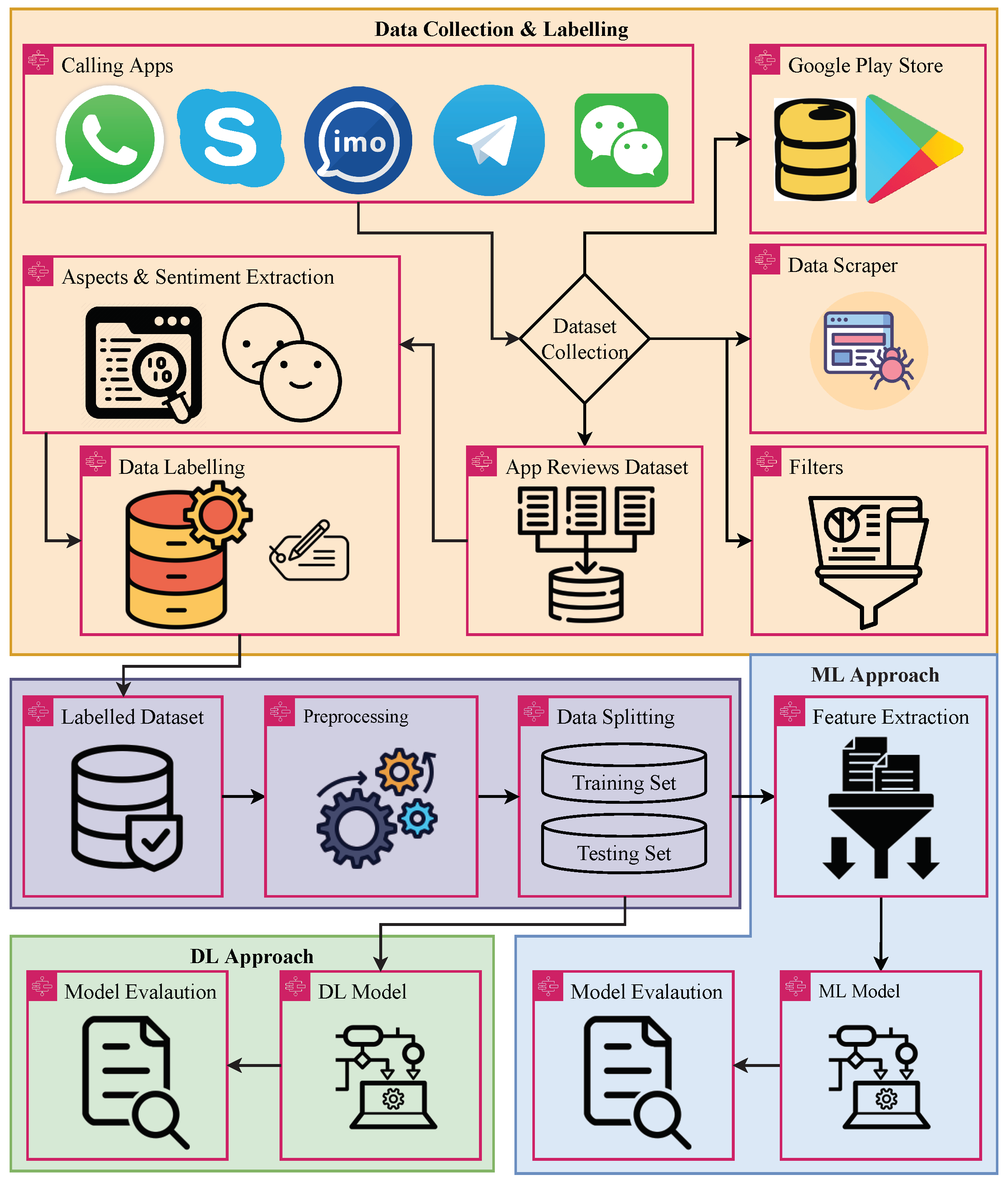
We also present an overall comparison between calling apps and suggest to users where they can find better services for their needs. The diagram of the proposed approach is shown in Figure 1. The first step is to collect the data for mobile apps. The data for five calling apps are collected to perform analysis. The data are collected from the Google Play Store using a web scraper. After extracting the dataset, aspect extraction and sentiment extraction are performed to label the dataset.

We proposed a supervised machine-learning approach for sentiment classification for which we required a labeled dataset; however, the original dataset was not labeled. We used VADER for data labeling with three sentiments negative, positive, and neutral. After data labeling, we used learning models. The LDA was used for aspect extraction, while VADER was used for sentiment extraction. The aspects and sentiments were used to label the dataset. The labeled dataset was further preprocessed to remove noise and unnecessary data.

In preprocessing, punctuation removal, numeric value removal, case conversion, stemming, and stopwords removal were performed. Preprocessing made the dataset clean and ready for split into training and testing sets with 0.8 to 0.2 ratios, where % of the dataset was used for the training of models and 20% of the dataset was used for the evaluation of models. The training and testing sample ratio is shown in

Table 3. Training and testing set count.

Dataset	Positive	Negative	Neutral
Training Set	19,554	9292	4037
Testing Set	4885	2324	1010
Total Count	24,429	11,616	5047

.

The training and testing sets were used for feature extraction techniques using TF-IDF, BoW, and Hashing Vectors. Machine-learning models were trained on these features, while deep-learning models do not require feature extraction techniques. Both machine-learning and deep-learning models were evaluated in terms of the accuracy, precision, recall, F1 score, and G-mean.

3.1. Dataset Description

The dataset used in this study consisted of reviews regarding the calling apps and was extracted from the Google Play Store. For that, this study used the ‘google_play_scraper’ Python library. Filters for the scrapper were set, such as the limit for the number of reviews set to 10,000, while the language was set to English. We targeted famous calling apps, such as Skype, WhatsApp, Wechat, Telegram, and IMO. For each app, we extracted 10,000 reviews, and the dataset contained a total of 50,000 reviews. The dataset was extracted on 25 March 2022 with the most recent reviews.

Table 4. Sample of the dataset.

Doc.	Review Id	User Name	User Image	Content
1	gp:AOqpT….	D.R	https://play…	Animated stickers take up WAY too much storage space.
2	gp:AOqpT…	La 201	https://play...	Have changed profile settings multiple times and still cannot see my profile photo
Doc.	Score	Thumbs Up Count	Review Created Version	at
1	3	539	8.6.0	13 March 2022
2	3	42	8.6.1	6 March 2022

shows a few samples from the collected dataset. It contains the review ID, username, user image, content (review text), score, thumbs up count, review created version, and date of the posted review.

3.2. Aspects and Sentiment Extraction

For aspect and sentiment extraction from app reviews, LDA and VADER techniques were used on the preprocessed data.

3.2.1. VADER

VADER uses a list of words to determine the context of the entire sentence, and the sentence is regarded as negative or positive. It is mostly used for the analysis of social media data. It takes an input and provides the output as the likelihood of that input being a positive, negative, or neutral remark. VADER gives a polarity score between −1 to 1 against the given text. If the score is less than or equal to −0.05, then it is a negative sentence, and if the score is greater than or equal to 0.05, then it is a positive sentence.

Table 5. Vader score range.

Sentiment	Score Range
Negative	Score ≤ − 0.05
Positive	Score ≥ 0.05
Neutral	Score > − 0.05 & Score < 0.05

shows the score range of VADER for awarding positive, negative, and neutral sentiments.

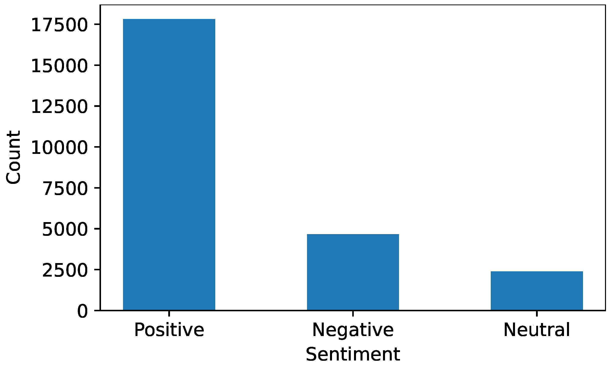
The collected dataset was labeled using VADER, and the number of positive, negative, and neutral sentiments vary significantly. The distribution of sentiments of the dataset is given in Figure 2.

3.2.2. Latent Dirichlet Allocation

This study used LDA for topic extraction from the documents [22]. LDA follows unsupervised classification on different documents to find natural groups of topics. It maps the probability distribution over latent topics by assuming that a document with similar topics will contain a similar group of words. LDA aims to classify the topics of documents based on the words in them. It is used to extract the specific aspects of the apps, such as calls, video, messages, working, updates, accounts, and apps. The process of topic extraction in the LDA can be defined as

$$P(z_1=j{Z}_t.w_t,d_t,.)\infty \frac{C_{w{}_{t}j}^{WT}+\beta }{{\sum }_{w=1}^W{C}_{w_j}^{WT}+W\beta }\frac{C_{d{}_{t}j}^{DT}+\alpha }{{\sum }_{t=1}^T{C}_{d_{{}_t}j}^{DT}+T\alpha }$$

(1)

where $C_{w{}_{t}j}^{WT}$ is the number of times a word appeared as the topic, $\beta$ is the per word topic distribution, W is the length of vocabulary, $C_{d{}_t}^{DT}j$ is the number of times a document appeared as the topic, $\alpha$ is per-document topic distribution, and T is the number of topics.

Table 6. Sentiments against topics.

Topic Name	Sentiment
	Negative	Neutral	Positive
account	4199	817	2866
app	341	278	9290
call	1922	816	2319
message	628	368	1944
update	1549	1023	1312
video	1110	663	4018
working	1867	1082	2680

shows the sentiments and aspects, which we extracted using VADER and LDA, respectively.

3.3. Preprocessing Techniques

Text reviews extracted from Google Play Store are in their raw form and may contain useless information. Preprocessing techniques were used to clean the dataset to extract the appropriate information, which helps to increase the performance of the learning algorithms [23].

3.3.1. Punctuation and Number Removal

While punctuation plays a major role in the construction of a sentence, it only increases the complexity in the learning of an algorithm [24]. Punctuation marks include a comma (,), full stop (.), semi-colon (;), colon (:), and more. The inclusion of unnecessary numbers, which play zero roles in the learning of text analysis and punctuation are eliminated to achieve an improved learning process.

3.3.2. Lemmatization and Stemming

To increase the accuracy rate of text analysis without increasing the learning complexity, Lemmatization and Stemming are both used to convert derivatives of a word into the base word. Stemming involves removing extra words, such as ‘s’ or ‘es’ to convert the word into its root form. However, in lemmatization, the base word prediction is made before the cutoff procedure of the derivative word, and in stemming, the extra words are removed first [25]. For example:

Studies $->$ Lemmatization $->$ Study

Studies $->$ Stemming $->$ Studi.

3.3.3. Stop Word Removal

Some words, mostly articles (such as “the”, “a” and “an”) or helping words (such as “is”, “am”, and “are”) carry no useful information and hence are removed to enhance the training process.

3.3.4. Conversion to Lower Case

To avoid having the same words analyzed twice, all words are converted to lowercase as the machines would read “machine” and “Machine” as separate words, which would eventually affect the training as well as classification performance.

Table 7. Data samples before and after preprocessing.

Before Preprocessing	After Preprocessing
Animated stickers take up WAY too much storage space.	anim sticker take way much storag space
Have changed profile settings multiple times and still cannot see my profile photo	chang profil set multipl time still see profil photo

shows the sample reviews before and after pre-processing.

3.4. Feature Extraction

Text can not be fed directly into the machine-learning models, and we need to transform the text into a numerical representation. For that, several feature extraction techniques are available, and this study uses three feature extraction techniques, such as BoW, TF-IDF, and Hashing.

3.4.1. Bag of Words

BoW is one of the commonly used techniques in NLP for extracting features from a given text. This method is considered the simplest and most flexible for feature extraction from documents. BoW converts the unstructured and amorphous data into a structured and organized form by changing the text data into an equivalent vector of numbers that represent the occurrence of words in a document. The BoW results on sample reviews after preprocessing are shown in

Table 8. The results of BoW on sample reviews.

Doc.	Anim	Chang	Much	Multipl	Photo	Profil	See
1	1	0	1	0	0	0	0
2	0	1	0	1	1	2	1
Doc.	Set	Space	Sticker	Still	Storag	Take	Time	Way
1	0	1	1	0	1	1	0	1
2	1	0	0	1	0	0	1	0

.

3.4.2. Term Frequency-Inverse Document Frequency

TF-IDF is a method for feature extraction that is commonly used for text analysis applications by giving scores to the words in a document. Using TF-IDF, the relevance of a word in a particular document can be statistically evaluated while considering the offset, i.e., the occurrence of that particular word in multiple documents. It is calculated by multiplying the Term Frequency (TF) metrics with the Inverse Document Frequency (IDF) metrics. Based on the result of multiplication, the relevance can be determined—for instance, the higher the score, the more relevant a word is to that particular document. TF-IDF can be represented as:

$$tfidf(t,d,D)=tf(t,d)·idf(t,D)$$

(2)

where t represents the word in a document d from a set of documents D.

TF-IDF results on sample preprocessed reviews are shown in

Table 9. The results of TF-IDF on sample reviews.

Doc.	Anim	Chang	Much	Multipl	Photo	Profil	See
0	0.377964	0.000000	0.377964	0.000000	0.000000	0.000000	0.000000
1	0.000000	0.301511	0.000000	0.301511	0.301511	0.603023	0.301511
Doc.	Set	Space	Sticker	Still	Storag	Take	Time	Way
0	0.000000	0.377964	0.377964	0.000000	0.377964	0.377964	0.000000	0.377964
1	0.301511	0.000000	0.000000	0.301511	0.000000	0.000000	0.301511	0.000000

.

3.4.3. Hashing Vector

A vectorizer that uses the hashing method to determine the token string name to feature integer index mapping is known as a hashing vectorizer. This vectorizer converts text documents into matrices by converting the collection of documents into a sparse matrix that holds the token occurrence counts. The benefit of using a hashing vectorizer is that there is no need to store the vocabulary dictionary in memory; it has extremely low memory scalability for huge data sets.

Table 10. The results of hashing on sample reviews.

Doc.	1	2	3	4	5	6
1	0.000000	0.333333	0.666667	0.333333	−0.333333	−0.333333
2	0.333333	0.333333	0.000000	−0.666667	−0.333333	0.000000
Doc.	7	8	9	10	11	12
1	0.0	0.0	0.000000	0.0	0.0	−0.333333
2	0.0	0.0	0.333333	0.0	0.0	−0.333333

contains the hashing results on sample preprocessed reviews when we selected 12 features.

3.5. Machine-Learning Algorithms

To classify the app reviews into their corresponding sentiments, we deployed several machine-learning models, such as SVM, KNN, DT, LR, and RF. These models were selected based on their performance for text classification reported in the literature. We deployed these models with their best hyper-parameter settings, which we found through the fine-tuning of models.

Table 11. Machine-learning model hyper-parameter settings.

Model	Hyper-Parameters	Hyper-Parameter Tuning
DT	max_depth = 300	max_depth = {50 to 500}
RF	n_estimators = 300, max_depth = 300	max_depth = {50 to 500}, n_estimators = {50 to 500}
XGBoost	n_estimators = 300, max_depth = 300, learning_rate = 0.8	max_depth = {50 to 500}, n_estimators = {50 to 500}, learning_rate = {0.0 to 1.0}
KNN	n_neighbors = 3	n_neighbors = {2 to 10}
SVM	Kernel = poly, C = 2.0	Kernel = {poly, linear, sigmoid}, C = {1.0 to 5.0}
LR	solver = liblinear, C = 2.0, multi_class = multinomial	Kernel = {liblinear, sag, saga}, C = {1.0 to 5.0}, multi_class = multinomial

shows the hyper-parameter settings for machine-learning models and the tuning range.

3.5.1. Decision Tree

DT is a powerful learning algorithm used for classification and prediction [26]. It is a tree-like structure in which each node/branch represents a feature from the dataset. These branches help to decide the outcome of a test data point. Each leaf node in the DT represents a class label to predict. To construct a DT, the entropy and information gain of each feature against the target variable are calculated to determine the precedence of feature nodes in the tree. After building the tree, test data points are predicted by traversing through the tree up to leaf nodes. The mathematical formulas for calculating the Entropy and information gain are presented in Equations (3) and (4), respectively.

$$E\left(S\right)=-\sum _{i=1}^c-p_{i}lo{g}_2{p}_i$$

(3)

$$IG\left(E\right)=1-\sum _{i=1}^c{p}_i^2$$

(4)

We deployed DT with one hyperparameter max_depth. This hyperparameter takes care of the depth of the tree. We set it to 300, which means that the tree will be restricted to 300-level depth. This hyper-parameter will help to reduce the complexity of the tree as shown in Table 11.

3.5.2. Random Forest

RF falls under the category of supervised machine-learning algorithms and has been used for both classification and regression problems [27]. In the case of classification, RF handles categorical data, while in the case of regression, it handles continuous data. RF is based on a large number of decision trees, where each DT gives a class prediction and the class with a maximum number of predictions becomes the model’s prediction. RF uses a method called bagging that allows each DT to randomly select a sample dataset to have different types of trees for better accuracy and minimum variance. Moreover, it uses feature randomness (a method in the ensemble), which increases diversification and decreases correlation among trees. RF can be represented as:

$$RFf{i}_i=\frac{{\sum }_{j\in alltrees}normf{i}_{ij}}{T}$$

(5)

where $RFf{i}_i$ is the importance of feature i that is calculated from all trees, $normf{i}_{ij}$ is feature i that is normalized in a tree j, and T is the number of trees. RF is used with two hyper-parameters as shown in Table 11. The n_estimator hyper-parameter defines how many decision trees will be in the RF voting procedure, and the max_depth hyper-parameter defines the depth of each DT. We used 300 decision trees, and each tree was restricted to 300 level depth.

3.5.3. Logistic Regression

LR is one of the commonly used machine-learning algorithms for classification. It is based on linear regression; however, the main difference is that it uses an activation function (typically Sigmoid) to map the output between 0 and 1. The output value between 0 and 1 represents the probability of the output class. That probability is later used to output a discrete value. LR can also be used for multi-class classification [28]. LR is mathematically represented as:

$$P=\frac{1}{1+e^{-}(a+bX)}$$

(6)

where P is the probability between 0 and 1, e represents the base of natural logarithms, a and b are defined as the parameters, and X is an independent variable. LR is also used with three hyper-parameters, such as solver, C, and multi_class as shown in Table 11. We used liblinear, sag, and saga optimizer. We used multi_class hyper-parameter with a multinomial value. We tuned LR with different settings to achieve significant results, and the best hyper-parameter settings are shown in Table 11.

3.5.4. Support Vector Machine

SVM is a supervised machine-learning algorithm that is used both for classification and regression. In SVM, data points are plotted in n-dimensional space, and then classification is performed by finding a hyperplane that segregates the data points well [29]. SVM works by identifying the right hyperplane and computing the distance between the nearest data points of the opposite class called support vectors. That distance is later used to draw/plot the margin between the hyperplane and data points to generalize the model. Two types of margins are used in SVM—namely, hard margin and soft margin. Hard margin performed well on the training set causing over-fitting and misclassification, while soft margin generalized the model well.

$${\beta }_0+{\beta }_1{X}_1+{\beta }_2{X}_2+\dots \dots +{\beta }_p{X}_p\ge 0$$

(7)

We used two hyper-parameters with SVM; one is the kernel, and the second is C. We used kernel with poly values, which performed better with the used dataset, and we used C, which is a regularization parameter with value 2.0 as shown in Table 11.

3.5.5. K-Nearest Neighbor

KNN is a supervised machine-learning algorithm that is used for both regression and classification. It predicts the class by computing the distance between the test data and all training points [30]. The distance between data points is usually computed using the Euclidean distance; however, Manhattan and Minkowski measures can also be used depending on the scenario. After computing the distance, the best K data points are selected, and then the prediction is performed based on the most repeated classes in K data points. The value of K is chosen based on the size of the dataset. This algorithm has no training step and is slow due to run-time computations to predict test data points. The Euclidean distance is represented as:

$$E_d=\sqrt{\sum _{i=1}^k(x_i-y_i)}$$

(8)

We used KNN with one hyper-parameter with n_neighbour. We used a value of 3, which means that KNN will focus on three neighbors and find the distances between them to classify the data.

3.5.6. XGBoost

XGBoost stands for extreme gradient boosting and is a distributed gradient boost machine-learning model. This is a tree-based ensemble model combining a number of decision trees. It trains decision trees in parallel to boost the accuracy. It is more scalable and portable compared to GBM. We used XGBoost with 300 n_estimators, which means that 300 decision trees were included in the decision process. We also used max_depth hyper-parameter with a 300 value, which means that each tree will grow to a max 300 level depth. The learning rate was also used with XGBoost with a value of 0.8, which helped to shrink the contributions of each decision tree.

3.6. Deep-Learning Algorithms

This section elaborates on the deployed deep-learning algorithms for the classification of reviews along with machine-learning algorithms. Deep-learning algorithms have been receiving attention recently due to their outstanding performance in classification and prediction. Researchers have been working on analyzing the performance of different deep-learning models [31], and in the same way, the proposed study also inspected several deep-learning models, such as LSTM, CNN, and GRU, in order to analyze their performances for sentiment classification. The architectures of all used models are discussed in Section 4.2.

3.6.1. Long Short-Term Memory

LSTM is a recurrent neural network used for the classification and prediction of time series data. It can process complete sequences of data instead of single data points. Typical recurrent neural networks (RNNs) are capable of processing current input data by using previous information. However, they have a lag in remembering long-term dependencies due to vanishing gradients, which is resolved by the introduction of LSTM [32]. This consists of three parts, i.e., the input gate, forget gate, and output gate.

The first part of LSTM decides whether the information from the previous timestamp is useful or not. The second part attempts to learn new information from the input. Furthermore, the third part passes the information from the current to the next timestamp. Like typical RNN, LSTM also has a hidden state of timestamps in addition to a cell state. The hidden state is known as short-term memory, while the cell state is known as long-term memory [33].

3.6.2. Convolutional Neural Network

CNN is a commonly used model for classification problems, particularly in image processing and textual classifications [34]. It takes the given data as an input and assigns weights to different aspects of the image that would help to differentiate the different types of data. CNN requires little data preprocessing as it takes raw data as the input and processes accordingly. Three types of layers, i.e., convolutional layers, pooling layers, and finally the fully connected layers, are used to form a CNN [35]. Convolutional layers are placed at the first stage to extract features from the input images, pooling layers are placed after the convolutional layers to decrease the size of feature maps and reduce computational costs, and finally, the fully connected layer is placed, which contains weights and biases in order to complete the classification process.

3.6.3. Gated Recurrent Unit

A gated mechanism in the RNN is called GRU, and it works similarly to an LSTM with a forget gate but has few parameters as it does not have an output gate. GRU was introduced after RNN and LSTM and provides improvements. The architecture is simple as it only has a hidden state, and thus it is faster at training. It takes the input and hidden state from the previous timestamp at the current input. After that, it processes the input and outputs a new hidden state for the next timestamp. In GRU, there is a two-step process to find the hidden state, i.e., the first step is where the hidden state is taken from the previous timestamp, which is later multiplied by the reset gate and the resultant value is called the candidate hidden state. Furthermore, in the subsequent step, the candidate state is later used to generate the currently hidden state [36].

3.6.4. Recurrent Neural Network

A recurrent neural network, an artificial neural network, is used for the prediction of sequential and time-series data. It uses previous input data from its memory to predict the current input data. Other deep neural networks are based on the assumption that input and output are independent, while an RNN uses the previous output for the upcoming inputs as they have some sort of sequence. In this way, an RNN makes predictions and is known as a multiple feed-forward neural networks as it passes information from one pass to another. It is widely used in applications of natural language processing, speech recognition, and image captioning. However, the vanishing gradient problem, a drawback in RNN, halts the learning of long data sequences [37].

3.7. Evaluation Metrics

Different evaluation metrics are used by researchers in order to measure the performance of algorithms. The evaluation metrics help in analyzing and comparing the overall performance of the algorithm and further assist in decision making. The proposed approach was evaluated against the following metrics.

3.7.1. Accuracy

Accuracy is defined as a performance measure used for classification types of algorithms in machine-learning models. It is defined as the ratio of correct predictions to total predictions. It is calculated as:

$$Accuracy=\frac{TP+TN}{TP+TN+FP+FN}$$

(9)

where TP indicates true positive, TN is true negative, FP is false positive, and FN is false negative. They are defined as:

• TP is true positive, which means that the model predicts the example as Yes, and the actual label of the example is also Yes.
• TN is true negative, which indicates that the model’s prediction is No, and the actual label of the example is also No.
• FP is false positive, which means that the prediction is Yes, but the actual label of the example is No.
• FN is false negative, which means that the model’s prediction of the example is No, but the actual label of the example is Yes.

3.7.2. Recall

Another measure for evaluating the performance of classification algorithms is known as recall. It calculates the true positive rate by determining the number of correct positives identified in the test data. The mathematical formula to calculate the recall is given in Equation (10).

$$Recall=\frac{TP}{TP+FN}$$

(10)

3.7.3. Precision

Precision is another well-known performance measure for classification algorithms. It calculates how many identified positives are correct in the test data. The ratio of positives to the total number of identified positives in the test sample is called precision. An algorithm will have a higher precision if it correctly predicts the positive samples well.

$$Precision=\frac{TP}{TP+FP}$$

(11)

3.7.4. F1 Score

F1 score is a performance metric for classification algorithms that helps to indicate the class imbalance. As it uses both precision and recall, it is considered more important than precision and recall alone. F1 is the harmonic mean of the precision and recall. If the precision and recall are high, then the F1 score will be high. If both are low, then it will also be low. It provides a medium value if one of them is low and the other is high.

$$F1Score=\frac{Precision\ast Recall}{Precision+Recall}$$

(12)

3.7.5. G-Mean

The G-mean is defined as the central values in the set of numbers calculated by taking the root of the nth degree of the product of n numbers in the set. A low G-mean represents the poor performance of models indicating that positive cases have been classified incorrectly, although negative cases are correctly classified. Therefore, the G-mean represents a balance between the classification of majority as well as minority classes. It is calculated as:

$$\left(\prod _{i=1}^n{x}_i\right)=n\sqrt{x_1{x}_2\dots \dots x_n}$$

(13)

where ∏ represents the product of a set of items, x represents the discrete item in the set, i denotes the index number of the items, and n denotes the total number of items.

4. Results

This section contains the results for the machine-learning and deep-learning models. It also presents the analysis of the apps’ aspects with respect to user sentiments. In the end, apps are categorized regarding their performance and different features.

4.1. Results of Machine-Learning Models

The machine-learning model results are evaluated in terms of the accuracy, precision, recall, F1 score, and G-mean using BoW, TF-IDF, and Hashing features.

Table 12. The results of machine-learning models using BoW features.

Model	Accuracy	Precision	Recall	F1 Score	G-Mean
SVM	0.91	0.89	0.88	0.88	0.88
DT	0.83	0.81	0.81	0.81	0.81
RF	0.85	0.83	0.79	0.81	0.81
LR	0.90	0.87	0.87	0.87	0.87
KNN	0.61	0.58	0.60	0.53	0.59
XGBoost	0.87	0.85	0.85	0.85	0.85

contains the results of the machine-learning models using the BoW features. The performance of models was good as SVM achieved a significant accuracy of 0.91 and a 0.88 F1 score. This is followed by LR, which obtained a 0.90 accuracy score and a 0.87 F1 score. The good performance of SVM and LR can be attributed to the large feature set. SVM and LR require a large feature set for a good fit, and the used dataset generates a large feature set using the BoW technique, which helps LR to achieve significant results.

Table 13. The results of models using TF-IDF features.

Model	Accuracy	Precision	Recall	F1 Score	G-Mean
SVM	0.91	0.90	0.89	0.89	0.89
DT	0.82	0.78	0.80	0.79	0.79
RF	0.84	0.83	0.76	0.79	0.79
LR	0.90	0.88	0.87	0.87	0.87
KNN	0.59	0.55	0.58	0.53	0.56
XGBoost	0.85	0.83	0.81	0.82	0.82

contains the results of machine-learning models using the TF-IDF features. The performance of the models is approximately similar to that of BoW, as SVM still has the highest accuracy score, followed by LR. Consistent better performance by the SVM and LR show that the linear models performed well on the dataset used in this study. KNN showed poor performance with BoW and TF-IDF features because it uses matching criteria between training and new data to make a prediction, and its performance was poor when the feature set was large.

The results using hashing features are given in

Table 14. The results using the hashing features.

Model	Accuracy	Precision	Recall	F1 Score	G-Mean
SVM	0.91	0.90	0.89	0.90	0.89
DT	0.82	0.79	0.79	0.79	0.79
RF	0.71	0.83	0.51	0.54	0.65
LR	0.90	0.88	0.87	0.88	0.87
KNN	0.63	0.58	0.60	0.56	0.59
XGBoost	0.85	0.83	0.79	0.81	0.81

, which indicates the variation in model accuracy and other metrics. Although the accuracy of the leading performers SVM and LR remains the same, a change in other models is observed. For example, the accuracy of RF reduced from 0.84 with TF-IDF to 0.71 when used with hashing features. On the contrary, KNN showed a marginal improvement of 0.4 in accuracy when hashing features were used. The performance of SVM was superior when used with hashing in comparison with BoW and TF-IDF because the hashing feature gives a more sparse feature set for learning models, which can be significant for linear models, such as SVM and LR. SVM achieved the highest F1 score of 0.90 using the hashing features.

Figure 3 shows the comparison between machine-learning models using BoW, TF-IDF, and hashing features. RF showed poor performance with hashing features, while the linear models improved their F1 score with hashing features.

Table 15. The per class scores for the machine-learning models.

SVC					DT
Features	Class	Precision	Recall	F1 Score	Features	Class	Precision	Recall	F1 Score
BoW	0	0.85	0.88	0.86	BoW	0	0.75	0.73	0.74
	1	0.84	0.80	0.82		1	0.78	0.83	0.80
	2	0.94	0.93	0.94		2	0.88	0.88	0.88
TF-IDF	0	0.86	0.89	0.87	TF-IDF	0	0.73	0.71	0.72
	1	0.88	0.80	0.84		1	0.75	0.81	0.78
	2	0.94	0.94	0.94		2	0.87	0.87	0.87
Hashing	0	0.88	0.89	0.88	Hashing	0	0.74	0.72	0.73
	1	0.89	0.83	0.86		1	0.76	0.79	0.77
	2	0.94	0.95	0.95		2	0.87	0.87	0.87
RF					XGBoost
Feature	Class	Precision	Recall	F1 Score	Feature	Class	Precision	Recall	F1 Score
BoW	0	0.85	0.72	0.78	BoW	0	0.82	0.80	0.81
	1	0.80	0.70	0.75		1	0.83	0.85	0.84
	2	0.86	0.94	0.90		2	0.90	0.91	0.91
TF-IDF	0	0.84	0.72	0.78	TF-IDF	0	0.91	0.78	0.80
	1	0.81	0.61	0.70		1	0.79	0.69	0.73
	2	0.84	0.94	0.89		2	0.87	0.91	0.89
Hashing	0	0.89	0.41	0.56	Hashing	0	0.89	0.78	0.80
	1	0.93	0.14	0.25		1	0.79	0.69	0.73
	2	0.68	0.98	0.80		2	0.87	0.85	0.87
LR					KNN
Feature	Class	Precision	Recall	F1 Score	Feature	Class	Precision	Recall	F1 Score
BoW	0	0.88	0.85	0.86	BoW	0	0.63	0.31	0.42
	1	0.81	0.83	0.82		1	0.29	0.74	0.42
	2	0.93	0.94	0.94		2	0.81	0.73	0.77
TF-IDF	0	0.88	0.86	0.87	TF-IDF	0	0.58	0.45	0.51
	1	0.85	0.79	0.82		1	0.26	0.62	0.36
	2	0.93	0.95	0.94		2	0.82	0.65	0.73
Hashing	0	0.87	0.85	0.86	Hashing	0	0.60	0.45	0.52
	1	0.84	0.82	0.83		1	0.30	0.63	0.40
	2	0.93	0.95	0.94		2	0.83	0.72	0.72

shows the per class score for each machine-learning model.

4.2. Experimental Results for Deep-Learning Models

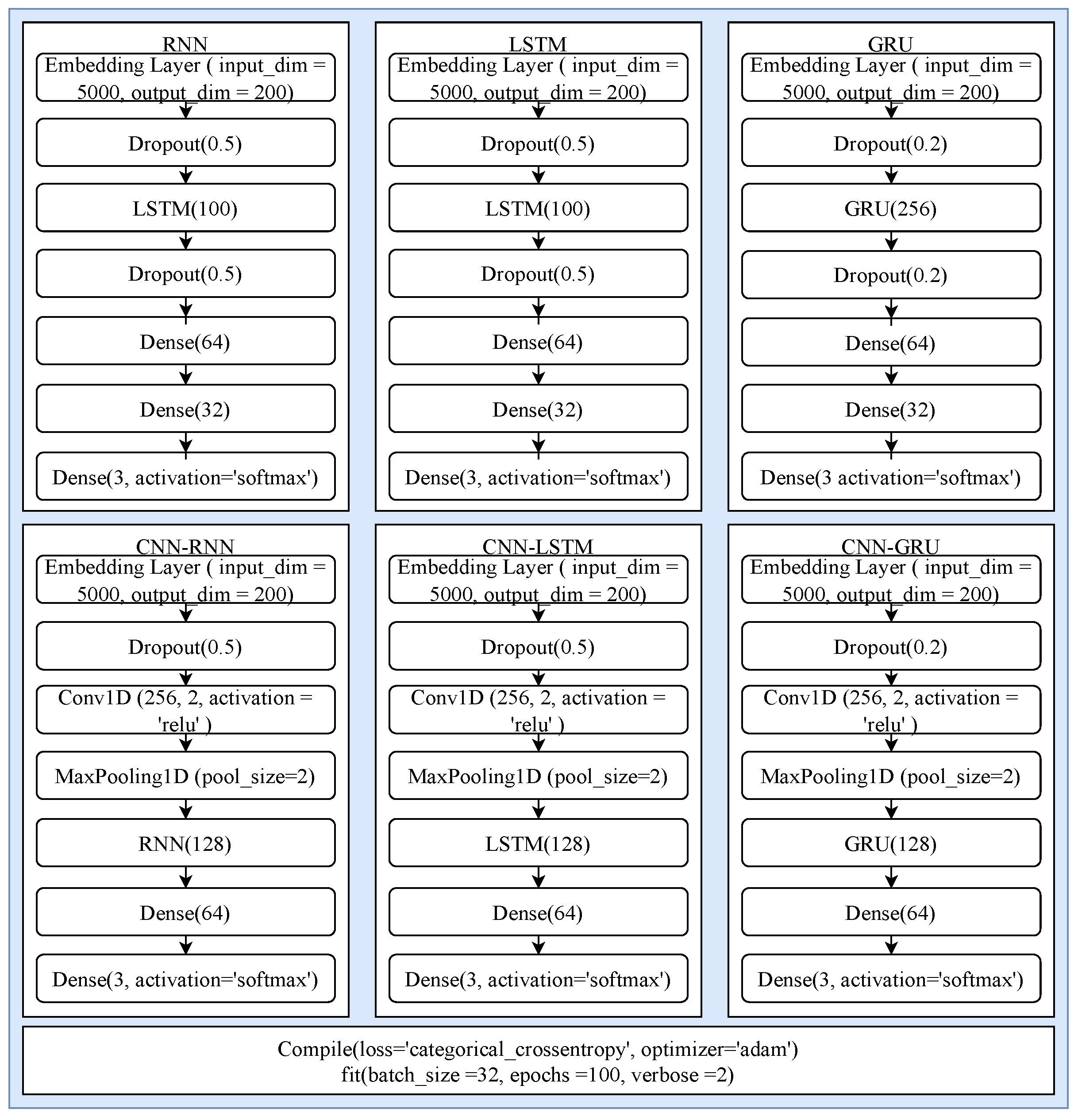
This study utilized LSTM, RNN, GRU, and CNN as well asd their combinations in comparison with machine-learning models. These models were deployed with their state-of-the-art architectures as shown in Figure 4. All models took text input through an embedding layer with a vocabulary size of 5000, and the output dimension size was 200. Each model consists of dropout layers with different dropout rates to reduce the complexity of computation and dense layers with a different number of neurons. As the end layer, each model consists of three neurons and a softmax activation function. All models are compiled using the categorical_crossentropy loss function because of the multi-class data and Adam optimizer. Each model is fitted with 100 epochs and a batch size of 32.

Table 16. Deep-learning model results.

Model	Accuracy	Precision	Recall	F1 Score	G-Mean
CNN	0.86	0.83	0.80	0.81	0.81
RNN	0.87	0.86	0.84	0.85	0.85
CNN-RNN	0.92	0.90	0.89	0.89	0.89
LSTM	0.92	0.91	0.89	0.90	0.90
CNN-LSTM	0.93	0.91	0.91	0.91	0.91
GRU	0.93	0.92	0.90	0.91	0.91
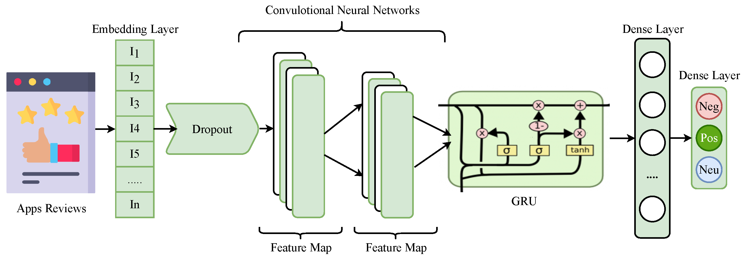
CNN-GRU	0.94	0.93	0.91	0.92	0.92

shows the results for the deep-learning models in terms of the accuracy, precision, recall, F1 score, and G-mean. The performance of all deep-learning models was significantly better in comparison with the machine-learning models. The experimental results reveal that GRU outperformed individual models for sentiment classification. For the better feature extraction capability of CNN, we combined CNN with GRU to break the traditional CNN-LSTM streak. This combination of CNN-GRU produced significant results as CNN feature mapping criteria helped to generate more correlated features for GRU to make more accurate predictions. The architecture of the proposed CNN-GRU is illustrated in Figure 5.

We used a CNN model with each recurrent architecture. CNN was used at the initial level for feature extraction, and then other models were used for the prediction. It can be observed that the performance of models improved after combining with the CNN. The highest accuracy was achieved by the CNN-GRU, which also outperformed the CNN-LSTM ensemble. The CNN-GRU obtained an accuracy score of 0.94, which was the highest of all the machine and deep-learning models used in this study. Its 0.92 F1 score was also the highest among all models. Similarly, LSTM also showed better performance when combined with CNN and obtained a 0.93 accuracy score and 0.91 F1 score.

The performance of top performance models from machine learning and deep learning is also elaborated in terms of the confusion matrix. SVM performed well in the machine-learning family, and the proposed CNN-GRU performed well regarding the deep-learning models. The confusion matrices for SVM and CNN-GRU given in Figure 6 indicate that SVM provided a total of 9161 correct predictions out of 10,000 predictions, while CNN-GRU outperformed with 9388 correct predictions.

Table 17. The per class score for the deep-learning models.

Model	Class	Precision	Recall	F1 Score
CNN-GRU	0	0.89	0.95	0.92
	1	0.93	0.81	0.87
	2	0.96	0.96	0.96
GRU	0	0.90	0.92	0.91
	1	0.91	0.81	0.86
	2	0.95	0.96	0.96
CNN-LSTM	0	0.88	0.94	0.91
	1	0.92	0.81	0.86
	2	0.96	0.96	0.96
LSTM	0	0.88	0.90	0.89
	1	0.88	0.80	0.84
	2	0.94	0.95	0.95
CNN-RNN	0	0.89	0.90	0.90
	1	0.88	0.81	0.85
	2	0.95	0.96	0.95
CNN	0	0.82	0.83	0.83
	1	0.79	0.64	0.70
	2	0.90	0.93	0.91
RNN	0	0.85	0.76	0.80
	1	0.85	0.81	0.83
	2	0.88	0.94	0.91

shows the per class score for the deep-learning models.

4.3. Analysis on Aspects of Calling Apps

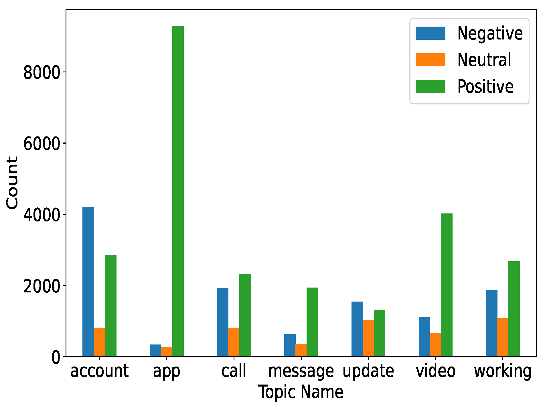
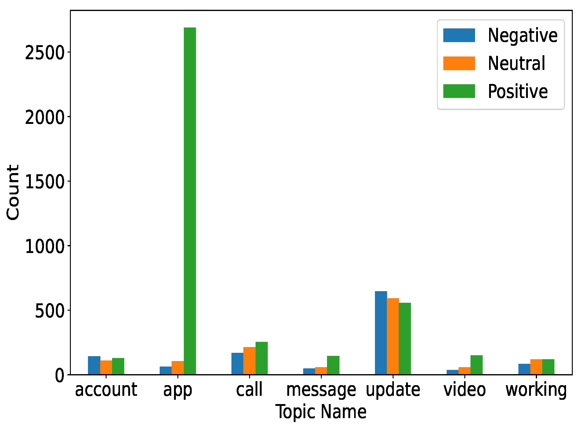
4.3.1. All Topic Sentiments

The topics considered for the sentiments were account, app, calls, messages, updates, videos, and the working of the apps. Three sentiments against which all the topics were evaluated were negative, positive, and neutral. It can be observed in Figure 7 that most of the positive sentiments were given to the apps. Similarly, videos also received a higher number of positive comments as compared to negative and neutral ones.

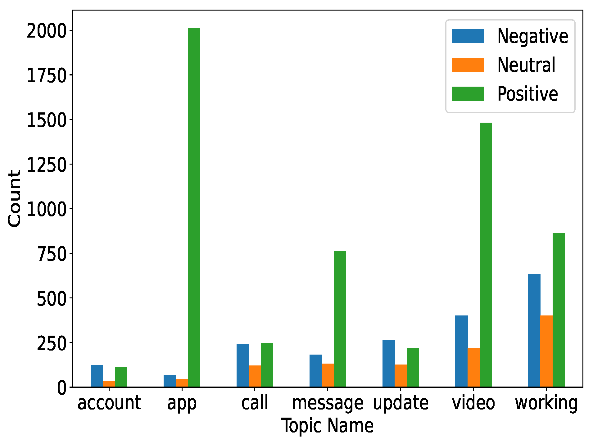
4.3.2. Overall Statistics of Calling Apps

Figure 8 shows the overall statistics of all the calling apps, such as IMO, Skype, Telegram, WeChat, and WhatsApp. It can be seen that IMO, Skype, and Telegram approximately received an equal number of positive counts. However, WeChat received a lower number of positive counts in contrast. Among all the calling Apps, WhatsApp managed to obtain the maximum number of positive sentiments, while the negative sentiments were few.

4.3.3. Sentiments for Individual Apps

This section contains the aspect-based analysis of each calling app. It also categorizes the app concerning different features according to people’s sentiments. In addition, the shortcomings of the apps are highlighted for improvement.

• Per Topic Sentiments for IMO
  It can be observed in Figure 9 that, among all the topics, IMO sustained more positive responses than negative or neutral ones against its app, account, calls, messages, video, and working. However, updates encountered a low number of positive sentiments.
• Per Topic Sentiments for Skype
  In the same way, it can be observed from Figure 10 that, among all the topics, Skype acquired a good number of positive responses against its app, call, messages, video, and working, whereas more issues were reported against accounts and updates of Skype.
• Per Topic Sentiments for the Telegram App
  Figure 11 shows the sentiment analysis on the calling app Telegram. We found that Telegram obtained the maximum number of positive responses against its app, call, messages, video, and working, while lacking a high number of positive sentiments against accounts and updates.
• Per Topic Sentiments for WeChat
  Likewise, the sentiment analysis on WeChat is represented in Figure 12. The graphical representation reveals that WeChat obtained a good number of positive responses for apps, calls, messages, updates, videos, and working features, while a lower number of positive sentiments were observed for accounts and updates. The distribution of the sentiments reveals that WeChat, as a whole, did not obtain good reviews, as the number of negative sentiments for the account was substantially large.
• Per Topic Sentiments for WhatsApp
  Figure 13 presents the distribution of positive, negative, and neutral sentiments regarding different features. The stats represent that WhatsApp obtained a good number of positive responses on apps, calls, messages, videos, and working. For the updates feature, on the other hand, the ratio of negative sentiments was high indicating an user unsatisfactory attitude regarding the updates offered by WhatsApp.

4.4. Discussion

Table 18. Aspect-based analysis of calling apps and their categorization.

Calling Apps	Account	Apps	Call	Messages	Update	Video	Working
IMO	Average	Good	Good	Good	Below Average	Good	Average
Skype	Below Average	Good	Good	Good	Average	Good	Good
Telegram	Below Average	Good	Average	Good	Below Average	Good	Good
WeChat	Below Average	Good	Average	Good	Below Average	Good	Good
WhatsApp	Average	Good	Average	Good	Below Average	Good	Good

shows the concluded points for calling apps where different apps are suggested with respect to the different features offered by the app and users’ satisfaction with those features. For this purpose, apps are categorized into good, average, and below-average classes regarding each feature. This helps users to select an appropriate app for the features they are looking for. According to the findings, Telegram, WeChat, and WhatsApp need to focus on call-related features because user sentiments rate it average, while Telegram, WeChat, and Skype need to work on their account policies. User sentiments rated this below average, and improvements could gain more users.

For classification, we achieved significant results using the hybrid approach CNN-GRU. This approach achieved significant accuracy because CNN extracts worthy features from the app reviews and passes them to the GRU to make accurate predictions, while other machine-learning models, such as LR and SVM, were also significant in terms of accuracy because the available feature set for machine-learning models training was large in size, which is a suitable environment for linear models.

4.5. Comparison with Existing Approaches

For a performance comparison, several other approaches were implemented in this study, and the results are presented in

Table 19. Comparison with other approaches.

Ref.	Year	Model	Accuracy	Precision	Recall	F1 Score	G-Mean
[38]	2018	Bi LSTM-CNN	0.90	0.90	0.90	0.90	0.9
[24]	2019	LR-SGDC	0.88	0.84	0.85	0.84	0.84
[8]	2020	LR + Chi2	0.91	0.90	0.88	0.89	0.89
[23]	2021	ETC + FU	0.82	0.86	0.70	0.74	0.78
[40]	2022	CNN-LSTM	0.88	0.88	0.86	0.87	0.87
[39]	2022	Attention CNN-LSTM	0.91	0.91	0.90	0.90	0.90
This study	2022	CNN-GRU	0.94	0.93	0.91	0.92	0.92

. Studies were selected for comparison due to the common nature of the research, as the selected studies also worked on sentiment analysis, aspect-based analysis, and app review classification. The study [38] worked on aspect-level text classification and deployed a Bi-LSTM-CNN model. The study [24] performed sentiment analysis for US airlines and proposed a hybrid machine-learning model by combining LR and stochastic gradient descent classifier (SGDC).

Similarly, [23] used an extra tree classifier (ETC) and feature union techniques to perform sentiment analysis on COVID-19 tweets. The study [8] worked on app review classification and proposed an approach using feature extraction, feature selection, and a machine-learning technique. The authors performed aspect-level sentiment classification in [39] by proposing an attention-based CNN-LSTM model. We re-implemented these previous studies’ approaches and performed experiments on our dataset for a fair comparison. The results indicate that the proposed approach performed better than these models and obtained a higher accuracy for sentiment classification.

4.6. Statistical T-Test

To show the significance of the proposed approach, a statistical significance test was also performed [41]. We deployed a statistical T-test on the results of proposed approaches vs. the machine-learning model results, deep-learning model results, and other approach results. The T-test evaluates the null hypothesis: If the T-test accepts the null hypothesis and rejects the alternative hypothesis, it means that the compared results are not statistically significant. If the T-test rejects the null hypothesis and accepts the alternative hypothesis, it indicates the compared results are statistically significant. The T-test gives output in terms of a T-statistic score (T) and critical value ($CV$), where, if the T score is greater than $CV$, then it rejects the null hypotheses and accepts the alternative hypothesis. The T-test results are shown in

Table 20. Statistically significant T-test.

Case	T	CV	Null Hypothesis
Proposed CNN-GRU vs. SVM (Hashing)	8.660	7.20 × 10${}^{-17}$	Rejected
Proposed CNN-GRU vs. CNN-LSTM	2.449	7.20 × 10${}^{-17}$	Rejected
Proposed CNN-GRU vs. [39]	4.899	7.20 × 10${}^{-17}$	Rejected

.

We selected the best cases in comparison with the proposed approach, such as from machine-learning models, SVM results with hashing were used, while the results of CNN-GRU were selected from the deep-learning models. From existing state-of-the-art studies, we used results from [39] for comparison. Table 20 shows that, for all cases, the t-test rejected the null hypothesis, which indicates that the results obtained from the proposed approach were statistically significant.

5. Conclusions

With the wide use of mobile phones, the demand for mobile apps has seen large development and deployment trends during the past few years. Of the several types of available apps on the Google Play store, calling apps, such as WhatsApp and Skype, are famous for their ease of sharing pictures, making video calls, sending audio messages, etc. However, each app has its pros and cons regarding different features, and feature analysis of these apps is often missed. This study presented an aspect-based analysis of famous mobile calling apps.

Five famous apps were considered in this regard, including IMO, Skype, Telegram, WeChat, and WhatsApp. A large-sized collected dataset was analyzed using LDA for aspect analysis and the account, app, call, message, update, video, and working features of these apps were analyzed. This kind of aspect analysis can help users to select an appropriate app regarding their desired features.

In addition, sentiment analysis was also conducted with a novel ensemble model comprising GRU and CNN, which provided a 94% sentiment classification accuracy. Aspect analysis revealed that IMO and Skype had the highest ratios of positive sentiments when the calling feature was considered, while for messages and video calls, all apps had equal user sentiments. From the perspective of user accounts, IMO and WhatsApp provided higher user satisfaction due to the ease of creating and managing accounts. Skype was on the top in terms of updating features.

In the future, we intend to work on finding appropriate suggestions for improving the quality of service for different calling apps regarding user sentiments. One of the limitations of this study is the size of the used dataset. We had only 50,000 reviews, and if we divide them into topics, the ratio is lower. We intend to extract more reviews in our future work. Analysis considering the region of the user is also intended because this has an impact on service quality. Another concern is that there can be slight overlapping in topics because, in many reviews, users talk about multiple features. User location can also have an impact on sentiment analysis, and thus, in our future work, we will analyze sentiment with respect to the user location.