Article

Super-Operator Linear Equations and Their Applications to Quantum Antennas and Quantum Light Scattering

School of Electrical Engineering, Tel Aviv University, Tel Aviv 69978, Israel
*
Author to whom correspondence should be addressed.
Appl. Sci. 2022, 12(17), 8498; https://doi.org/10.3390/app12178498
Submission received: 11 April 2022 / Revised: 18 August 2022 / Accepted: 22 August 2022 / Published: 25 August 2022

Abstract

:
In this paper, we develop a resolvent method for super-operator equations with applications in quantum optics. Our approach is based on the novel concept of a linear super-operator acting on the Hilbert subspace of vector or scalar linear operators satisfying physically reasonable commutation relations. The super-operator equations for the electromagnetic (EM) field operators are formulated for the problems of quantum antenna emission and quantum light scattering by a dielectric body. The general solution of super-operator equation is presented in terms of the classical resolvent. In contrast to the classical case, it includes the ancillary components associated with the quantum noise even in the absence of absorption. The reason for this lies in the energy exchange between different spatial regions with various bases for the field presentation (which looks like losses or gain from the point of view of the correspondent region). A number of examples (a two-element dipole antenna, a plane dielectric layer, and a dielectric cylinder with a circular cross section) which demonstrate the physical mechanism of the appearance of noise are considered. It is shown that antenna emission or scattering transforms the coherent properties of quantum light. This leads to a new way of controlling coherence in a direction-dependent manner, a feature that can be useful in various applications of quantum technologies, including quantum radars and lidars, and quantum antennas.

1. Introduction

The scattering of a quantum electromagnetic (EM) field is related to the wide research area stimulated by potential applications in quantum computing and quantum informatics [1,2,3,4], quantum communications [4,5], quantum circuits [6], quantum antennas [7,8,9,10,11,12,13], quantum radars and lidars [14,15,16], sensing and measurements [17]. Currently, this field is in the initial stages of its development. Probably, it will evolve along a path rather similar to classical electrodynamics and macroscopic antenna theory [18,19]. On the other hand, from time to time, it is expected to encounter fundamental problems with origins that are completely quantum and that do not have any classical analog (as one of such examples, one may note the manifestation of photon entanglement [1,2,3,4,5]). One of the first stages in the development of the field consists of the exact analytical solutions of some model problems. This phase has started: the quantization of some exact analytical solutions of Maxwell equations obtained via the separation of variables (spherically layered multimode systems [20] and parabolic mirrors [21]) has been given.
As a parallel method of development, one can mention high-frequency physical diffraction theories (for example, quantum diffraction by apertures [22,23]) and their comparison with the physics of simple quantum-optical devices (beam-splitters, interferometers, etc. [24]). You can expect that this phase will stimulate the establishment of universal numerical techniques, based on the so-called “discretization” of Maxwell equations (such as the methods of characteristic modes [25,26,27,28,29,30], integral equations [31], finite elements [32], finite differences [33], etc.). In the process of their making, the methods of classical electrodynamics will be an important element of the framework. As a promising step in this direction, one may note the quantization of characteristic modes [34,35]—the preliminary version of integral equations [36]—a numerical approach based on the synthesis of time-domain finite element analysis with the canonical quantization technique [37].
Further progress in the design of quantum devices often necessitates an accurate solution of the problems of quantum field scattering. From a naïve point of view, the canonical field quantization looks like a formal replacement of classical fields by the corresponding operators, which act in the Hilbert space of wavefunctions (quantum states) and satisfy appropriate commutation relations [38,39]. However, the problem is not limited to the replacement of classical values with the corresponding field operators. In classical electrodynamics, we note a widely used class of methods (including integral equations), in which the whole system is decomposed into a number of spatial regions. For example, for the scattering from a dielectric body, the integral equation is often formulated with respect to the field inside the body. The outside field is expressed through the inside one via an integral over the body volume. Another example is an antenna, defined as a device which transforms the near field to the far field and vice versa. Such transformation is formally described by special integral relations based on the Green theorems [18]. In the case of quantum field, the situation changes dramatically. The quantum field alongside the field operators (which satisfy Maxwell equations) is characterized by the quantum state ( Ψ -function). The introduction of partial regions requires a decomposition of the wavefunction of the whole space into those of the partial regions. The observable values are defined as expectation values of the corresponding operators with respect to the quantum state of the system [38,39]. The field operators which are related to the given partial region act on the correspondent partial wavefunction. As a result, the scattering of the quantum EM field will be accompanied by the appearance of entanglement in the new basis.
The formal description in our paper will be given in terms of super-operators. The super-operator A ¯ is defined as a mapping of one area of quantum operators onto another one (in contrast to an operator, which defines the correspondence between two areas of functions). The formation of the mathematical theory of super-operators [40] began simultaneously with the emergence of quantum mechanics (the von Neumann equation and Lindblad master equation [41] are related to the typical class of super-operator equations for the matrix of density). In this paper, we introduce another concept of a linear super-operator, which allows us to apply the integral equations theory to the scattering of quantum light and quantum antennas.
It is important to make a note on the role of losses in our concept of a super-operator. The losses in conventional quantum language mean the exchange of energy between the considered system (“small” system) and large external system described as a bath [42]. The “small” system is considered from the point of view of an open system. If we speak about thermal losses, the energy exchange means the energy transformation to heat. In this case, the bath takes the form of a thermal reservoir. Such an exchange is accompanied by the production of noise, without which the correct commutation relations become unattainable. A similar situation takes place for an active medium: the gain is necessarily accompanied by the noise [43,44,45].
The modeling of quantum light scattering and quantum antenna emission in this general language leads to the description of every partial region as an open quantum system. It continues the concept formulated previously for quantum antennas [7]: the emission of a quantum antenna looks like a loss from its point of view (in spite of the absence of any absorption). Therefore, the external space with the receiver and the environment is considered as a bath of non-thermal origin. This allows us to apply the general strongly developed theory of open systems [42] to quantum antennas.
The subject of this paper is an application of the super-operator concept to the scattering of quantum light and quantum antennas. The paper is organized as follows: the general form of the super-operator integral equation will be given in Section 2. The noise term will be considered and proved to have the form that guarantees the required form of commutation relations in the general case. The application of the developed approach to the quantum antennas will be given in Section 3. The manifestations of the noise component in the transmission reflection and scattering by the circular cylinder will be considered as examples in Section 4 and Section 5, respectively. The conclusion and future perspectives are discussed in Section 6.

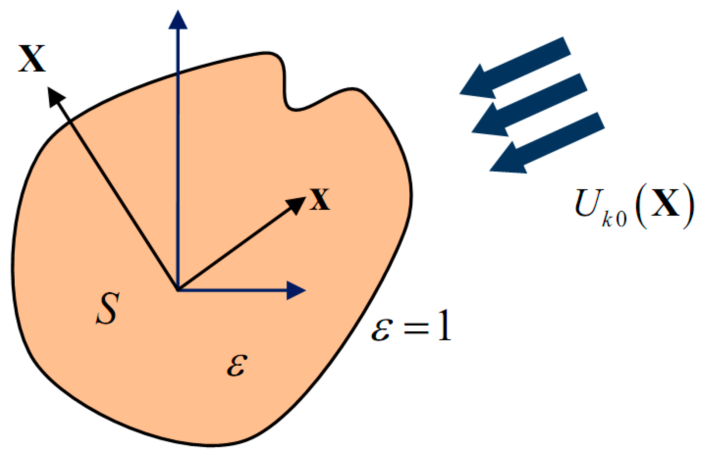
2. Super-Operator Integral Equation for Scattering of Quantum Light by a Dielectric Body

2.1. Preliminaries

The super-operator equation in our case may be written as
( I ¯ ν A ¯ ) x ^ = f ^ ,
where ν is a spectral parameter (c-number), I ¯ is the unit super-operator, and x ^ and f ^ are operators in the space of quantum states ( x ^ is unknown, while f ^ is given).
The formal solution of Equation (1) is x ^ = R ¯ ν f ^ = ( I ¯ ν A ¯ ) 1 f ^ , where R ¯ ν is the resolvent, which in our case is a super-operator too. As mentioned above, the operators x ^ and f ^ must satisfy the required commutation relations. Therefore, we encounter the main difference between the super-operator equations of the type (1) and their classical operator analogs. In contrast to the classical case, the resolvent R ¯ ν acts not on the whole Hilbert space, but on the subspace limited by the commutation relations. As will be shown below, the action of the resolvent is able to remove the operator x ^ out of the defined subspace. As a result, one may obtain a mathematically exact, but physically incorrect solution with inadequate commutation properties. In other words, Equation (1) is related to ill-posed mathematical problems and should be regularized for its correct application. Its regularization will be given in this paper. It is based on the introduction of the ancillary components, which are associated with a special type of quantum noise.
The configuration under consideration is shown in Figure 1. We decompose the operator of the longitudinal electric field into positive and negative frequency components [38,39] as E ^ x , t = E ^ + x , t + E ^ x , t and present it in the frequency domain as
E ^ + x , t = i 0 U ^ k x e i ω k t d k ,
where ω k = k c , k is wavenumber, and c is light velocity in free space. A similar representation for E ^ x , t is obtained from Equation (2) via its Hermitian conjugation. It will be useful to introduce the vector potential A ^ x , t = A ^ + x , t + A ^ x , t which is coupled with the field by the relation E ^ x , t = t A ^ x , t . For the spectral density, we have the Helmholtz equation
2 U ^ k + k 2 ε x U ^ k = 0 ,
where the symbol designates two-dimensional Laplacian and
ε x = ε , x S 1 , x S .
The spectral density operator U ^ k x plays a role in the complex amplitude of the classical case. Like in the classical case, it satisfies boundary conditions at the boundary of the body (continuity of the tangential components of the field) and radiation condition. Following standard techniques of classical electrodynamics, one can write the solution in terms of the resolvent. For the positive frequency component of the field inside the body, the solution reads
U ^ k x = U ^ k 0 x k 2 ε 1 S Γ x , x ; k U ^ k 0 x d x ,
where Γ x , x ; ν is the resolvent kernel defined by Equation (A5). The negative frequency component U ^ k + x inside the body may be obtained via the Hermitian conjugation of Equation (5). It is generally accepted to write the resolvent as a function of the spectral parameter ν = k 2 ε 1 as in Equation (A1). We made the transformation Γ x , x ; ν Γ x , x ; k in Equation (5) (and will use it in future) because wavenumber will play the role of a variable of integration in different relations. One can find the short reminder of resolvent theory for the classical Fredholm equations in Appendix A.
If the inside field is known, the outside field may be found via the integration over the body volume
U ^ k X = U ^ k 0 X k 2 ε 1 S g X , x U ^ k x d x ,
where X S . For the negative frequency component, the equation may be found via the Hermitian conjugation of Equation (6). Equations (5) and (6) look like the complete solution of the scattering problem: they satisfy the Helmholtz equation over the whole space, boundary conditions and radiation conditions.
In contrast to the classical case, we need to add the commutation relation, which reflects the bosonic origin of the EM field. The commutation relation is local; thus, it may be used in the ordinary form for homogeneous medium. As shown in Appendix B, it reads
U ^ k x , U ^ k + x = k 2 c π ε x Im g x , x δ k k
In fact, it is obtained from the relation for homogeneous dielectric space by replacing ε ε x .

2.2. Commutation Relation and Noise Component

As one can see, it is impossible to consider Equations (5) and (6) as a solution for the field operators because they do not satisfy the correct commutation rule (7). We will expand it next and make the suitable modifications, which will lead to the physically correct solution. First, let us explain the reason for such a situation. To this end, we will calculate the commutator U ^ k x , U ^ k + x for operators U ^ k x   and   U ^ k + x defined by Relation (5) and its Hermitian conjugate. The final result is
U ^ k x , U ^ k + x = k 2 c π ε Im Γ x , x ; k δ k k .
One can find the details of the calculations in Appendix C. As one can see, Equation (8) does not agree with the correct Equation (7) because of the appearance of the resolvent kernel Γ x , x ; k instead of the Green function g x , x . This is a manifestation of scattering, which means that the classical resolvent technique cannot be directly transferred to the quantum case.
We will now consider their special regularization, the main idea of which is the addition of the ancillary noise components. As a result, Equations (5) and (6) are modified in the following way:
U ^ k x = U ^ k 0 x k 2 ε 1 S Γ x , x ; k U ^ k 0 x d x + F ^ k x ,
where F ^ k x is the noise field. For the negative frequency component inside the body, the solution may be obtained via the Hermitian conjugation of Equation (9). The concept of noise looks similar to the lossy beam-splitter [44]; however, in our case, their physical origin is different (the thermal losses are absent). We have for the noise field F ^ k x = F ^ k + x = 0 (the symbol F ^ k + x here and in future denotes the Hermitian conjugation of the noise field). The noise field operators commute with field operators U ^ k 0 x , U ^ k 0 + x and satisfy the commutation relation
F ^ k x , F ^ k + x = c k 2 π ε δ k k Im Γ x , x ; k g x , x .
The noise field may be presented in the form of a series over the eigenstates u n x defined by Equation (A2):
F ^ k x = n f ^ k n u n x
and similar for the Hermitian conjugate operator. The pair f ^ k n , f ^ k n + is the creation–annihilation operator for noise mode with index n at the given frequency ω = k c . The commutation relations for them stem from Equation (10) and have the form
f ^ k n , f ^ k n + = c k 2 ν π ε δ n n δ k k Im 1 ν n ν ν n .

2.3. Observable Values

We have considered quantum light scattering from the point of view of open quantum systems (for example, applied to the modeling of lossy beam splitter in [44]). The concept of composite quantum systems is used in it as a main framework. The composite quantum system is considered as a set of two (or more) subsystems, whose statistical properties completely define the behavior of the total system. For example, the two subsystems may be two atoms in molecules, two modes in the EM field, or two elements in an electrical circuit, etc. In our case, the fields in two geometrical regions (the area inside the dielectric body and the whole outside space, near-field and far-field zones of antennas, etc.) play the role of subsystems. As a starting point, the Hilbert space of a composite system defined as a tensor product S = S ( 1 ) S ( 2 ) of Hilbert spaces of its subsystems S ( 1 ) and S ( 2 ) (superscripts 1 and 2 indicate the areas inside and outside the dielectric body, respectively) should be introduced.
The incident field is produced by the set of external sources distributed over the whole space. Such a set may be considered as a composite quantum system and characterized by the density matrix, which is the operator in the state space S . We will decompose the total source into two subsystems, in which the first one consists of sources outside the body and the second consists of inside ones. We will assume that the sources of different subsystems are uncorrelated. Therefore, the total density matrix takes the form of a tensor product of the density matrices of the partial regions: ρ = ρ 1 ρ 2 . Due to the noise component, the operators U ^ k x , U ^ k + x for the field inside the body act on the total space S . For the calculation of observable values, the field operators are conveniently present in the form of the tensor products. Operator (9) will have the form
U ^ k x = U ^ k 0 x I ^ 2 k 2 ε 1 S Γ x , x ; k U ^ k 0 x I ^ 2 d x + I ^ 1 F ^ k x ,
similar to the negative frequency field U ^ k + x (operators I ^ 1 , 2 denote the identity super-operators in the subspaces S ( 1 , 2 ) ).
For an arbitrary operator O ^ acting on the total space S , the observable value is O ^ = T r O ^ ρ . Assuming that the fluctuating part is in vacuum state, we obtain for the observable field:
U ^ k x = U ^ k 0 x k 2 ε 1 S Γ x , x ; k U ^ k 0 x d x
(with no support of fluctuations). For the intensity O ^ x = U ^ k + x U ^ k x , we have
O ^ x = U ^ k + x U ^ k x = U ^ k 0 + x R ¯ + R ¯ U ^ k 0 x + F ^ k + x F ^ k x 0 ,
where R ¯ ( ) = ( ) + ν S Γ x , x ; k ( ) d x is the resolvent operator, and 0 denotes averaging over the vacuum state 0 0 . As one can see from Equation (15), the second term describes the vacuum fluctuations of the intensity of the field inside the body due to the exchange of its energy with the outside space. This shows that the scattering of quantum light is necessarily accompanied by the fluctuations. This looks similar to the relation between fluctuations and dissipation (“fluctuation-dissipative theorem” [42]). Therefore, one can speak here about “fluctuation-scattering theorem”. Its origin is completely quantum: the second term in Equation (15) vanishes in the classical limit. Another origin of the noise component is the thermal radiation of the body environment. In this case, we are speaking about a thermal bath instead of a photonic one. Note that the statement of the quantum light scattering problem without accounting for any type of reservoir becomes physically contradictive.

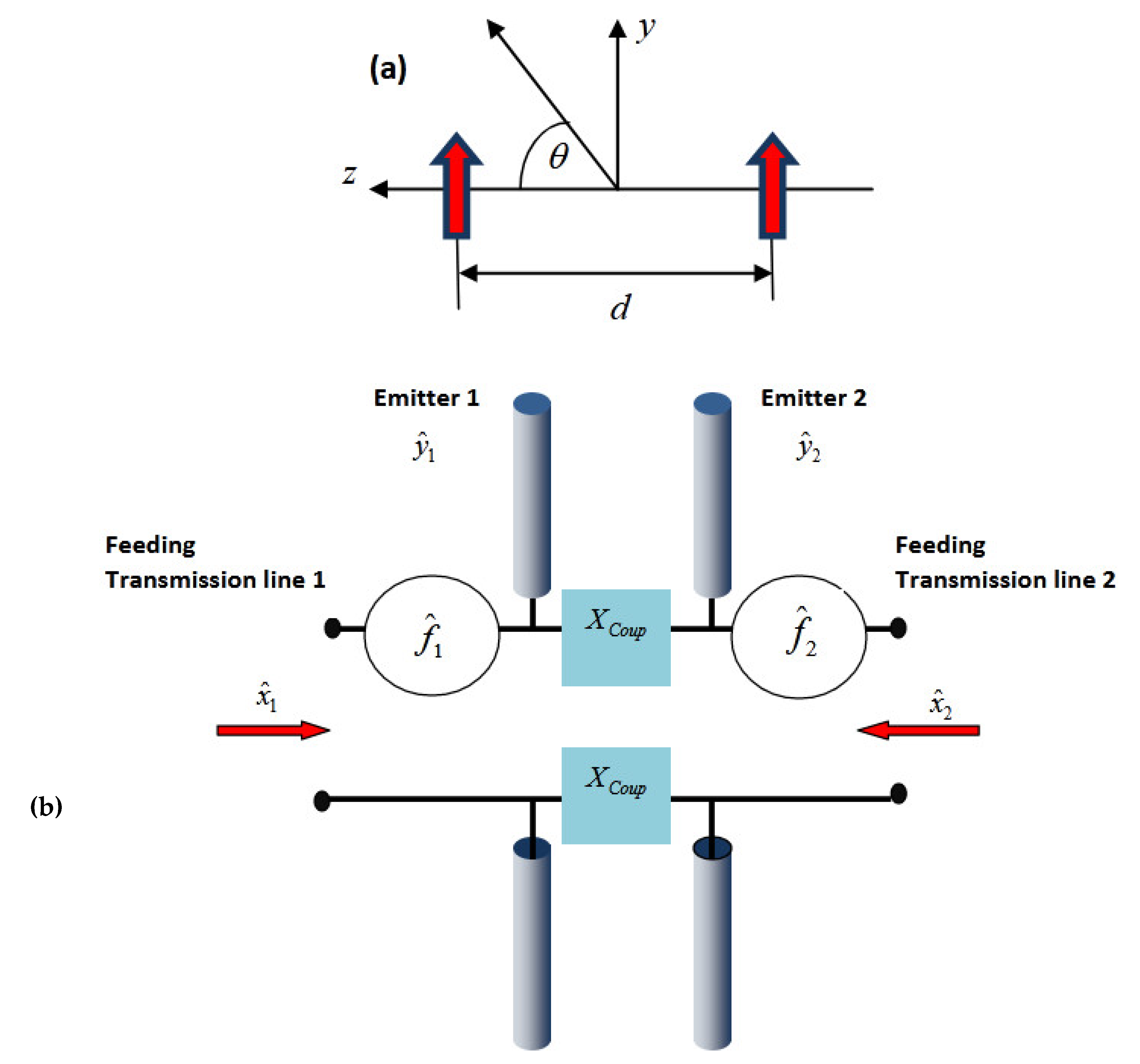
3. Application to the Quantum Two-Element Antenna Array

The purpose of this section is to present an application of the super-operator concept to a quantum two-element array of the dipole emitters shown in Figure 2. This type of antenna is widely used in classical radio engineering and its application in super-resolving quantum radars was proposed in [15].

3.1. Quantum Noise and Commutation Relations

The incident field (incoming modes) and emitted field (outgoing modes) may be described by the 4D columns of creation–annihilation operators x ^ 1 , x ^ 2 , y ^ 1 , y ^ 2 and x ^ 1 i , x ^ 2 i , y ^ 1 i , y ^ 2 i , which are coupled via the resolvent matrix ( S ¯ -matrix) as
x ^ 1 x ^ 2 y ^ 1 y ^ 2 = r t 1 t 2 t 3 t 1 r t 3 t 2 t 2 t 3 r t 1 t 3 t 2 t 1 r Resolvent   matrix x ^ 1 i x ^ 2 i y ^ 1 i y ^ 2 i .
Here, x ^ 1 , 2 is the pair of outgoing mode creation operators at the first and second feeding transmission lines, y ^ 1 , 2 is the pair of outgoing creation operators at the first and second dipole emitters, and the additional subscript i indicates the incoming mode at the corresponding channel. We assume that all channels are identical; therefore, the reflection coefficient r is the same in all channels. A similar relation may be written for the annihilation operators via the Hermitian conjugation of Equation (16).
The emitting properties of the antenna are characterized by the array factor [18]. For the quantum case, it becomes the photonic operator. Its positive frequency component in the yz plane is:
AF + θ = y ^ 1 e i ϕ + y ^ 2 e i ϕ ,
where ϕ = k d cos θ + β , with θ as the polar angle in the spherical system with origin placed at the antenna geometrical center, and β as the phase shift. We assume that the system is lossless and reciprocal; thus, matrix S ¯ is unitary [46,47]. It leads to the coupling relations between its elements:
r 2 + t 1 2 + t 2 2 + t 3 2 = 1 ,
Re r t 1 + t 2 t 3 = 0 ,
Re r t 2 + t 1 t 3 = 0 ,
Re r t 3 + t 1 t 2 = 0 .
The operators satisfy the ordinary bosonic commutation relations x ^ 1 , x ^ 1 + = x ^ 2 , x ^ 2 + = 1 , x ^ 1 i , x ^ 1 i + = x ^ 2 i , x ^ 2 i + = 1 , y ^ 1 , y ^ 1 + = y ^ 2 , y ^ 2 + = 1 , y ^ 1 i , y ^ 1 i + = y ^ 2 i , y ^ 2 i + = 1 , and all other pairs of operators commute.
It is convenient for antenna applications to transform the equivalent four-port network into a pair of coupled two-port networks. This entails the decomposition of the whole system into a pair of subsystems, each of which is described on a different basis (actually, the whole antenna decomposes into a pair of dipole emitters and feeding transmission lines). To this end, Relation (16) may be rewritten as
x ^ = A ¯ x ^ i + B ¯ y ^ i ,
y ^ = B ¯ x ^ i + A ¯ y ^ i ,
where A ¯ = r t 1 t 1 r and B ¯ = t 2 t 3 t 3 t 2 are 2D blocks of the S ¯ -matrix in Relation (16). Matrix A ¯ describes the coupling between emitters with their corresponding feeding lines, as well as mutual transmission line coupling. Matrix B ¯ describes the coupling of every emitter with the free space, as well as the mutual coupling of emitters due to their near fields. The vectors x ^ , x ^ i , y ^ , y ^ i are 2D columns of annihilation operators x ^ = x ^ 1 x ^ 2 , x ^ i = x ^ 1 i x ^ 2 i , and similar for y ^ , y ^ i .
For the classical field, we obtain Equations (22) and (23) for the corresponding classical values instead of operators. In our case, the incoming field appears only at the first and second channels. In this case, for classical field we should take y ^ i = 0 (this means that the second subsystem is excited only via the coupling with the first one). However, such assumption becomes unphysical in the quantum case. The reason being the fundamental absence of empty channels in the quantum field. The non-excited channels in the quantum case should be considered as channels with zero photons (which means that y ^ i = 0 ). However, it is impossible to ignore them because they are responsible for thermal and vacuum EM fluctuations, the omission of which contradicts the correct commutation relations.
To facilitate the application of the resolvent theory, we should transform the systems (22) and (23) in the following way. Relation (23) is equivalent to
y ^ = B ¯ x ^ i + f ^
where A ¯ y ^ i = f ^ . The first term on the right-hand side describes the excitation of the dipole emitters, while the second term corresponds to their coupling with the external space. From the point of view of the emitters it looks like energy is being lost, while it is not related to dissipation. Such “effective losses” may be positive and negative (the “effective gain” for receiving antenna). The operator f ^ = f ^ 1 f ^ 2 commutes with x ^ , x ^ i , and f ^ = 0 . The commutation relations for this operator stem from the commutation relations for y ^ i , and using Equations (18) and (19), may be written as
f ^ 1 , f ^ 1 + = f ^ 2 , f ^ 2 + = 1 t 2 2 t 3 2 , f ^ 1 , f ^ 2 + = t 2 t 3 t 3 t 2 .
The non-zero right-hand side of Equation (25) manifests the non-unitarity of the matrix block B ¯ (in spite of the unitarity of the total S ¯ -matrix in Relation (16)). The commutation Relation (25) completely coincides with the corresponding relations of the lossy beam-splitter [44], where the right-hand sides are stipulated to produce quantum noise due to the dissipative processes. This is the reason to associate operator f ^ with quantum noise too, in spite of the absence of any dissipation. This is a result of the separate description of antenna emission and antenna feeding taking into account their interaction only at the final step. It is clear that the noise operator acts on the wavefunction of the second subsystem. This leads to the modification of the Thevenin-like equivalent scheme [18]: in contrast to the classical case, this creates a pair of additional noise sources (see Figure 2b).

3.2. Transformation of the Statistical Properties of Quantum Light via the Quantum Antenna

Let us consider the calculation of the observable characteristics of quantum light. The antenna emission state is characterized by the wavefunction, which reads in the tensor form as
Ψ = n 1 n 2 C n 1 , n 2 n 1 : ψ 1 n 2 : ψ 2 = n 1 , n 2 C n 1 , n 2 n 1 n 2 ,
where n α : ψ α denotes a state with n photons in mode number α = 1 , 2 , and C n 1 , n 2 are arbitrary coefficients which satisfy the normalization condition. The directional dependence of the field properties is defined by the array factor given by Relation (17).
For our future purposes, it is convenient to move the directional dependence to the wavefunction and use the spatially independent array factor related to the antenna feed point. The situation is similar to the relation between the Schrodinger and Heisenberg pictures of quantum mechanics (with angle instead of time). Let us introduce the unitary operator
^ θ = m , n e i m n ϕ m n n m ,
where ϕ = k d cos θ + β / 2 . The wavefunction of the field in the far zone may be introduced as
Ψ r a d = ^ θ Ψ = m n e i m n ϕ C m n m n .
An arbitrary operator in such picture is transformed by the relation F ^ ^ + F ^ ^ . In particular, the array factor will be transformed by the following relation
AF + θ AF + = ^ + θ AF + θ ^ θ = y ^ 1 + y ^ 2 .
Let us turn now to the analysis of the antenna coupled with the feeding channels, as shown in Figure 2b. Here, we introduce the Hilbert space of a composite system defined as a tensor product S = S ( x ) S ( y ) of Hilbert spaces of subsystems S ( x ) and S ( y ) (superscripts (x) and (y) are related to the feeding lines and emitting dipoles, respectively). We will introduce the pure quantum state of light in the form of the tensor product Ψ = Ψ x Ψ y . The states Ψ x , Ψ y are given by
Ψ x = n 1 n 2 C n 1 , n 2 n 1 : ψ 1 n 2 : ψ 2 , Ψ y = 0 : ψ 3 0 : ψ 4 ,
where n α : ψ α denotes the state with n photons in the mode number α = 1 , 2 , 3 , 4 , similar to Equation (26), and C n 1 , n 2 are arbitrary coefficients which satisfy the normalization condition.
The operator y ^ defined by Relation (24) acts in the space S ( y ) . It may be represented as an operator in S using a form of the tensor product. We have
y ^ = I ^ x B ¯ x ^ i + f ^ I ^ y ,
where I ^ x , y are identity operators in space S ( x , y ) . As an example, let us calculate the observable y ^ + y ^ S , which may be associated with an analog of intensity for the scattering by a dielectric body considered in Section 3 (the symbol S means averaging over the state Ψ = Ψ x Ψ y ). Taking into account that for the noise in the vacuum state f ^ = 0 and using Relations (30) and (31), we obtain
y ^ + y ^ S = Ψ y B ¯ x ^ i + B ¯ x ^ i Ψ y + 0 f ^ + f ^ 0 .
The second term in Relation (32) corresponds to the support of fluctuations. It may be transformed to 0 f + f 0 = t 2 2 + t 3 2 = 1 r 2 t 1 2 .
Let us consider an example of the antenna excitation by a single photon in each feeding line. The wave function of the incident field is Ψ = Ψ x Ψ y = 11 00 . Assuming t 1 t 2 + r t 3 = 0 and t 1 t 3 + r t 2 = 0 , we obtain that the antenna interaction with the feed lines transforms the wavefunction to
Ψ = Ψ x 00 + 00 Ψ y ,
where
Ψ x = 2 r t 1 20 + 02 + r 2 + t 1 2 11 ,
Ψ y = 2 t 2 t 3 20 + 02 + t 2 2 + t 3 2 11 .
As one can see from Equations (33)–(35), the feeding of the quantum antenna leads to an entanglement of quantum states of the external sources and the emitting dipoles. Following Equation (28) for the transformation of the wavefunction (35) to the radiative form, we obtain
Ψ y r a d = 2 t 2 t 3 20 e 2 i ϕ + 02 e 2 i ϕ + t 2 2 + t 3 2 11 .
Let us consider a special example where we assume that the antenna is perfectly matched to the feed lines ( r = 0 ) and the feed lines are uncoupled ( t 1 = 0 ). In this case, the entanglement between the antenna emission and antenna feeding becomes suppressed, in spite of the entanglement between the two emitters. As a result, we have the wavefunction
Ψ r a d = i 2 00 20 e i ϕ + 02 e i ϕ r a d .
As one can see from Equation (37), in this special case, two photons will be emitted with a probability of 0.5 from one of the emitters, while the probability to emit one photon from one of the emitters is equal to zero. This shows the fundamental property of quantum antennas: the process of antenna emission transforms the statistical properties of light (in particular, it creates the inter-mode entanglement in the far field zone).
The angular distribution of the emitted field is characterized by the first- and second-order correlation functions at the same point in the far zone. The corresponding expressions for the quantum state (37) read
G 1 θ = sin 2 θ ( r a d Ψ AF + AF Ψ r a d ) = 2 sin 2 θ ,
G 2 θ = sin 4 θ ( r a d Ψ AF + AF + AF AF Ψ r a d ) = 4 sin 4 θ cos 2 ϕ =       4 sin 4 θ cos 2 1 2 k d cos θ + β .
The first-order coherence is equal to the intensity of the emitted field. Its directive properties are equal to those of a Hertzian dipole. This results from the summation of partial powers emitted by each emitter without any interference mechanism for the quantum state (37). In contrast, the second-order coherence exhibits the narrow lobe-like directive properties, as follows from Equation (39). The angular dependence of the second-order correlation exhibits a set of identical lobes separated by zeros. Such behavior was predicted for the first time for the N element antenna array in another quantum state in [10]. The number of lobes increases and their width decreases with increasing k d . The direction of the lobes is controllable by varying the phase shift β . It facilitates a method of electrically angular scanning by means of quantum antennas. Such ability may be important for applications in quantum radars and lidars [15].

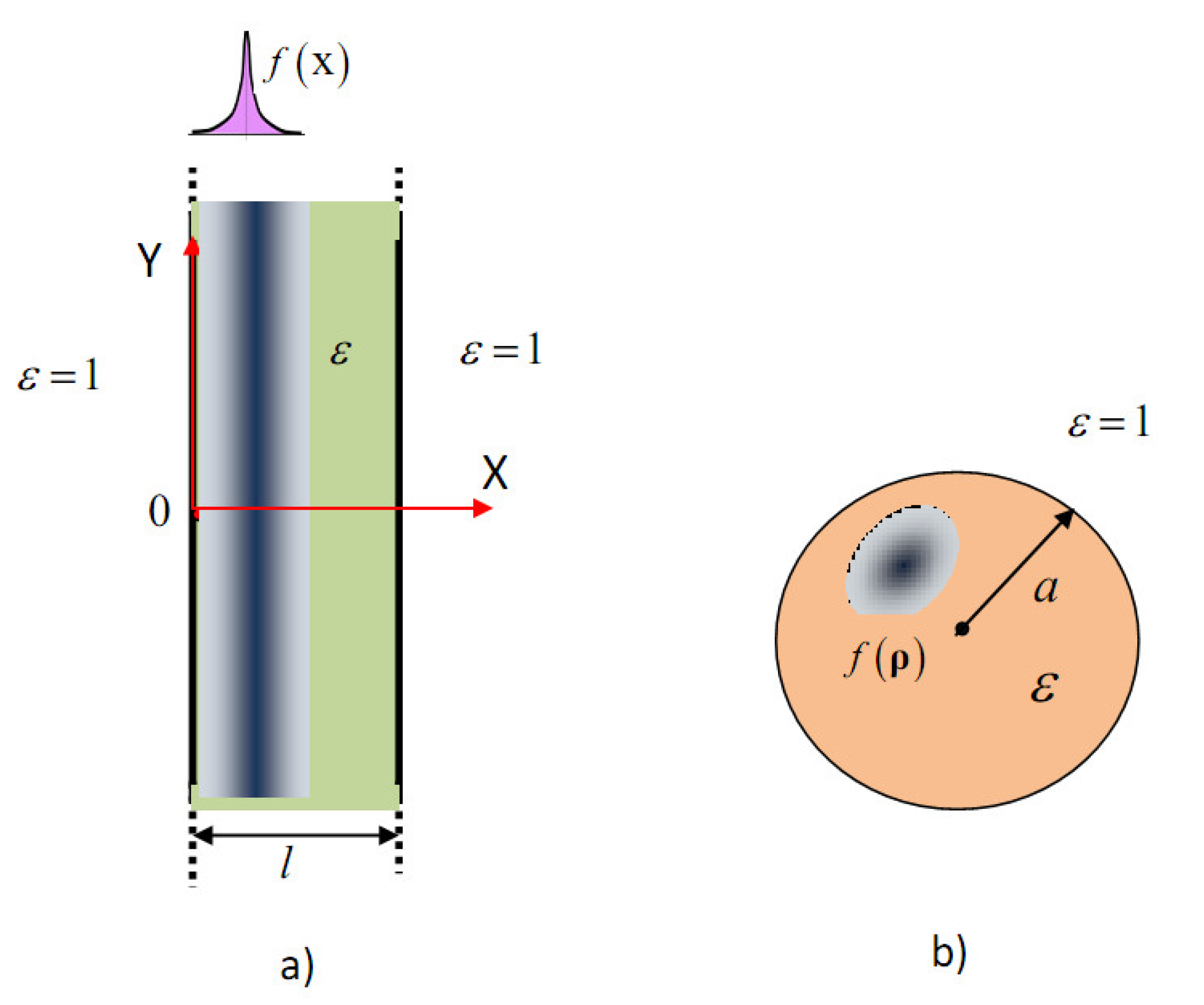
4. Planar Dielectric Layer: Reflection–Transmission

The problem’s geometry is shown in Figure 3a. The system is excited by the external current f x distributed inside the dielectric layer along the x-axis and vanishing outside the layer. Therefore, the field is dependent only on one variable, x. The equation for the total field becomes
d 2 U k d x 2 + k 2 ε x U k = f x ,
where the permittivity ε x = ε inside the layer and ε x = 1 outside it. The boundary conditions for the unknown field stem from the boundary conditions for the tangential component of the electric field at the boundaries of the dielectric layer [19,46]. The problem should be supplemented by the radiation condition at x < 0 and x > l.
The total field may be represented as a sum of incident and reflected–transmitted fields: U k = U k 0 + U ˜ k . The incident field U k 0 is produced by the same source in the absence of the dielectric layer. Therefore, it satisfies equation d 2 U k 0 d x 2 + k 2 U k 0 = f x . For the reflected–transmitted field inside the layer, we have equation d 2 U ˜ k d x 2 + k 2 ε U ˜ k = ν U k 0 , where ν = k 2 ε 1 , and d 2 U ˜ k d x 2 + k 2 U ˜ k = 0 outside. Our goal is to calculate the resolvent of the integral equation
U ˜ k x = w k 0 x + ν 0 l g x , x U ˜ k x d x ,
where w k 0 x = ν 0 l g x , x U k 0 x d x . It is an analog of the general integral Equation (A1) for the 1D case (where g x , x = e i k x x / 2 i k ).
We can represent the unknown field as
U ˜ k x = ν 2 i k ε 0 l e i k ε x x U k 0 x d x + A e i k ε x + B e i k ε x , 0 x l ,      C e i k x , x > l ,      D e i k x , x < 0 ,
where A, B, C, and D are unknown constant coefficients. Using boundary conditions, we obtain a system of four linear equations
A + B D = 1 ε f + , ε A B + D = f + , A e i Φ ε + B e i Φ ε C e i Φ = e i Φ ε ε f , ε A e i Φ ε B e i Φ ε C e i Φ = e i Φ ε f ,
where Φ = k l , Φ ε = k ε l , f ± = ν 2 i k 0 l e ± i k ε x U k 0 x d x . System (43) is easily solvable. We need only two of unknowns, for which we have
A = ξ ε f + e 2 i Φ ε r f , B = ξ ε r f + f ,
where r = 1 ε 1 + ε 1 is the Fresnel coefficient for normal incidence and ξ = r e 2 i Φ ε 1 r 2 e 2 i Φ ε 1 .
Using Solution (44) together with Relation (42), we obtain the solution inside the layer in the canonical form
U ˜ k x = ν 0 l Γ x , x ; k U k 0 x d x ,
where the function
Γ x , x ; k = 1 2 i k ε e i k ε x x +     1 2 i k ε 1 r 2 e 2 i k ε l r e i k ε x + x + r 2 e i k ε x x + 2 l + r 2 e i k ε x x 2 l r e i k ε x + x 2 l
may be associated with the resolvent kernel of the integral operator and used for the analysis of commutation relation for the case of the dielectric layer. In agreement with general Equation (A5), we have Γ x , x ; k = Γ x , x ; k . Therefore, the commutation relation may be written as
A ^ + x , t , E ^ x , t = i π ε Γ x , x ; k k d k .
The support of the first term in Equation (46) gives the correct commutation relation. For the analysis of all other terms, let us consider the analytical continuation to the complex k-plane. All these terms are analytical functions with the exception of the poles defined by the equation in which r 2 e 2 i k ε l = 1 . All these poles are located in the lower half-plane. The functions are exponentially decreasing in the upper half-plane. Therefore, this component of Integral (47) may be closed in the upper half-plane and gives zero contribution to the commutator. Thus, the noise components of the fields disappear in agreement with [44].

5. Scattering by the Dielectric Cylinder

The purpose of this section is to find the resolvent for the dielectric cylinder of the circular cross section. To this end, we will solve the Helmholtz equation:
2 ρ 2 + 1 ρ ρ + 1 ρ 2 2 φ 2 U k + k 2 ε ρ U k = f ρ
with permittivity ε ρ = ε inside the layer and ε ρ = 1 outside. The right-hand side in (48) is associated with the external force arbitrarily distributed inside the cylinder. The unknown function satisfies the boundary conditions for the longitudinal component of the electric field at the boundary of the cylinder [19,47] and radiation condition outside.
The scattered field may be represented similarly to Equation (42) by
U ˜ k ρ = i ν 4 S H 0 1 k ε ρ - ρ U ˜ k 0 ρ d ρ +     ν n A n J n k ε ρ e i n φ , 0 ρ a
and
U ˜ k ρ = ν n B n H n 1 k ρ e i n φ , ρ a ,
where A n , B n are unknown coefficients which can be founded from boundary conditions. We will omit their calculations here (see Appendix D).
The final result for the field inside the cylinder is
U ˜ k ρ = ν S Γ ρ , ρ ; k U k 0 ρ d ρ ,
where
Γ ρ , ρ ; k = i 4 H 0 1 k ε ρ ρ + δ g ρ , ρ ; k ,
δ g ρ , ρ ; k = i 4 n W n k J n k ε ρ J n k ε ρ e i n φ φ ,
And
W n k = H n 1 k a H n 1 k ε a ε H n 1 k a H n 1 k ε a H n 1 k a J n k ε a ε H n 1 k a J n k ε a .
Relation (51) expresses the scattered field through the incident field inside the cylinder in the canonical integral form. Therefore, Relation (52) may be associated with the resolvent kernel of the integral operator and used for the analysis of commutation Relation (18) and the existence of noise.
Let us transform Relation (18) for the dielectric cylinder to the form, and similarly transform Equation (47) for the 1D dielectric layer (integration over the whole axis instead of the positive semi-axis with the subsequent integration in the complex plane). It is necessary to note that here the situation dramatically changes compared with the 1D case. The difficulty lies in the non-analyticity of the function W n k given by Relation (54) in the complex k -plane (this function is multi-valued with a branch point at k = 0 in contrast to the dielectric layer case). One can see from well-known identities J n x = 1 n J n x , H n 1 e j π x = H n 2 x , and H n 2 e j π x = H n 1 x that it is natural to place the cut in the complex k -plane along the negative semi-axis (jagged line in Figure 4). It is easy to show that W n x = W n e i π x and W n k goes to zero if k in the upper half-plane. Thus, for Quantity (53), we obtain the relation between two branches of complex variable k :
δ g ρ , ρ ; k = δ g ρ , ρ ; e i π k .
The integration in Relation (47) for the cylinder may be transformed into an integral over contour C
A ^ + x , t , E ^ x , t = i π ε C Γ x , x ; k k d k
with its contour passing below the branch cut, as shown in Figure 4.
The contribution of the first term in Relation (52) to Relation (56) gives the conventional value of commutator without any noise components. However, in contrast to the 1D single-layer case (Section 4), the second term’s contribution does not vanish. The reason being the impossibility to close the contour in the upper half-plane, where the function tends to be zero (to do it one we need to cross the branch cut). This term is responsible for the noise current given by Equation (10).

6. Conclusions

In summary, we developed a novel method for the modeling of quantum light scattering and quantum antennas. It is formulated in terms of a linear super-operator defined as an operator in the Hilbert space, which acts in the subspace of quantum state operators, satisfying the physically appropriate commutation relations. It is shown that in the general case, the naïve quantization via the formal exchange of the classical values by the corresponding operators leads to an ill-posed super-operator problem. The reason is that the action of super-operator A ¯ may throw the result outside of the required subspace, which violates the correct commutation relations. In order to satisfy them, one needs to complete the regularization of the super-operator equation.
The proposed regularization technique is based on the introduction of ancillary channels, which are associated with the novel type of quantum noise, whose origin is not related to any dissipation of energy. The regularized super-operator equation has the form A ¯ E ^ = E ^ 0 + Q ^ , where Q ^ is a noise operator. Its form and commutation relations are determined in this paper. In general case, the super-operator equations may be solved numerically. Exact analytical solutions exist for special types of configurations. Sometimes, the approximate analytical solution is promised (for example, the perturbation technique). The solution of the regularized super-operator equation may be expressed in terms of classical resolvent, which may be found by one of the methods of classical computational electromagnetics [48].
Simple applications of the theory are considered using several examples (two-element dipole quantum antenna, reflection–transmission in a 1D dielectric layer, and scattering by a dielectric cylinder). It is shown that a special noise is produced via the exchange of energy between the body and the external space. From the “point of view” of the dielectric body, the process of multimode scattering looks like losses (or equivalent gain, if the energy enters from outside) in spite of the absence of any heating or real physical amplification. As a result, the exchange of energy is accompanied by a noise similar to that in systems with real physical dissipation. Thus, it becomes possible to speak about the general “fluctuation-scattering theorem” similar to the well-known “fluctuation-dissipating theorem”: the scattering of the quantum field is accompanied by fluctuations. In partial cases, a similar mechanism manifested itself in a parallel-plane beam splitter [49] and time lenses [50]. In [49], the initial photon state as a product of number states in both modes is considered. It was shown that the lossless feature due to beam-splitter coupling created a noise in the photon number of each mode in spite of the total photon number being invariant and noise-free.
The theory developed in this paper may be generalized for many other scattering problems (different types of quantum antennas, scattering from 3D dielectric bodies, or dielectric bodies with different types of environments, etc.). It suggests a new method for using scattering analysis as a tool for controlling the statistical properties of quantum light. It may be applied to various problems posed by quantum technologies, metamaterials [51], radars and lidars [14,16], quantum circuits, and nanoantennas [52,53,54,55].

Author Contributions

Conceptualization, G.S. and A.B.; Formal analysis, G.S. and A.B.; Writing—original draft, G.S. and A.B.; Writing—review & editing, G.S. and A.B. All authors have read and agreed to the published version of the manuscript.

Funding

This research was funded by NATO grant number NATO SPS-G5860 and by H2020, project TERASSE 823878.

Institutional Review Board Statement

Not applicable.

Informed Consent Statement

Not applicable.

Data Availability Statement

Not applicable.

Conflicts of Interest

The authors declare no conflict of interest.

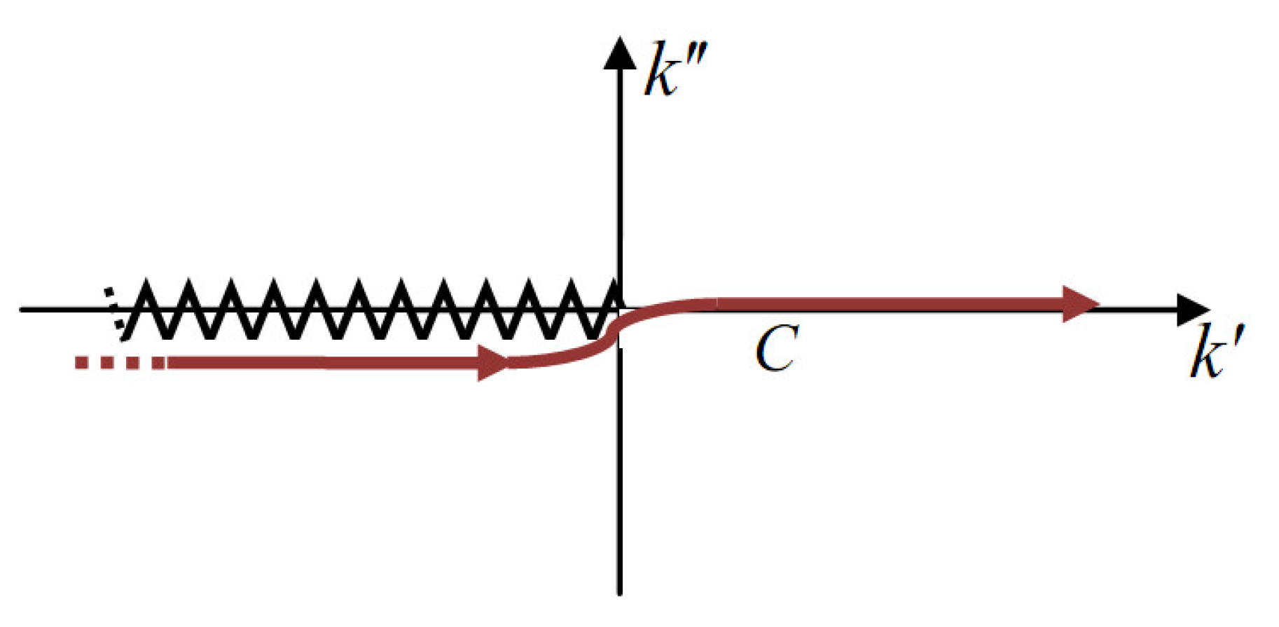
Appendix A. Resolvent Theory for Classical Operators

The Fredholm integral equation of the second type in general form may be written as [56]
E x ν S g x , x E x d x = E 0 x ,
where E x is an unknown function, ν is a given parameter, and E 0 x (right-hand term) and g x , x (kernel) are a priori given functions. The eigenfunctions u n x of the integral Fredholm operator are defined by the homogeneous version of Equation (A1):
u n x = ν n S g x , x u n x d x .
For the scattering problems, the kernel of the integral equation is the Green function of the Helmholtz equation. For the two-dimensional (2D) case g x , x = i 4 H 0 1 k x x where H 0 1 x is the Hankel function of the zero order and the first type, as one can see, the integral operator kernel is symmetric g x , x = g x , x but non-Hermitian ( g x , x g x , x ). Regarding the validity of the resolvent approach for this class of integral equations, in principle, the eigen-functions for non-Hermitian operators may not generate the complete basis system, and may not exist at all. However, the operator A ¯ ( ) = S g x , x ( ) d x has some fundamental properties due to the special form of its kernel. First, the kernel has a weak singularity (integrable in the ordinary sense). Second, we can split the kernel g x , x into the real and imaginary parts and write A ¯ ( ) = A ¯ R ( ) + i A ¯ I ( ) , where subscripts R, I mean real and imaginary components, respectively. The singular component of operator A ¯ ( ) is its real (Hermitian) part, while its imaginary part is regular. Thus, unbounded inverse I ¯ ν A ¯ R 1 ( ) exists. Combining these two facts means that operator A ¯ ( ) is a weak perturbation of Hermitian operator A ¯ R ( ) [57]. For weak perturbations of Hermitian operators, one can use the fundamental mathematical theory of pseudodifferential operators in Sobolev spaces [57] (in particular, the theorems on basis properties). For real k and u x L 2 S , we have Im S S g x , x u x u x d x d x < ( L 2 S (which is a space of Lebesgue squared integrable functions). In such cases, the operator A ¯ ( ) is a bounded operator acting from L 2 S to Sobolev space H 2 S . Such an operator is a completely continuous (compact) one. This means that the eigenvalues ν n exist as non-zero, and lie in the upper half-plane ( Im ( ν n ) > 0 ), and the resolvent set is non-empty [57].
It is easy to prove the orthogonality of eigenfunctions in the following form
S u n ( x ) u m ( x ) d x = δ m n
using the standard procedure. To that end, we should take Equation (A2) with index m, multiply it by u n x , multiply (A2) by u m x , subtract one from another, and integrate over S. The kernel may be represented as
g x , x = n 1 ν n u n x u n x .
The kernel
Γ x , x ; ν = n 1 ν n ν u n x u n x
is referred to as the resolvent kernel of integral Equation (A1) [58].
The kernel (A4) and resolvent kernel are coupled via the Hilbert–Schmidt Relation [58]:
g x , x + Γ x , x ; ν = ν n 1 ν ν n ν n u n x u n x .
The general solution of Equation (A1) may be efficiently presented in terms of the resolvent operator. It may be written as
E ν x = E ν 0 x + ν S Γ x , x ; ν E ν 0 x d x .
One more identity will be useful in our future consideration:
1 ν n 1 ν m S u n ( x ) u m ( x ) d x = 2 i S S Im g x , x u n ( x ) u m ( x ) d x d x .
It may have a proven similarly to orthogonality Relation (A3); however, instead of Relation (A2) with index m, its complex conjugated equation should be used.

Appendix B. Quantization of Free Electromagnetic Field on A Cylindrical Basis

The purpose of this Appendix is the derivation of commutation Relation (7). We will consider the homogeneous space with permittivity ε using the cylindrical basis. Let us present the positive frequency component of the operator of vector potential in the form
A ^ + x , t = 0 1 ω k U ^ k x e i ω k t d k .
A similar relation may be written for the negative frequency component of the electric field:
E ^ x , t = i 0 U ^ k + x e i ω k t d k ,
where U ^ k x , U ^ k + x is the pair of Hermitially conjugated operators of spectral density. The problem is finding the commutation relation for the operators of spectral density, which gives the canonical bosonic commutation relation for the EM field.
Let us present the operator of spectral density as a superposition of cylindrical waves:
U ^ k x = i E ˜ k n = 1 i n J n k ρ e i n φ b ^ n k ,
where E ˜ k = ω k k / 4 π ε is a normalization coefficient, J n x is Bessel function, and b ^ n k , b ^ n k + is a pair of creation–annihilation operators of cylindrical modes. We assume that they satisfy the conventional bosonic-type commutation relation
b ^ n k , b ^ n k + = δ n n δ k k .
Let us consider the commutator U ^ k x , U ^ k + x . Substituting in it Relation (A11) and its Hermitian conjugate, we obtain
U ^ k x , U ^ k + x =    ω k ω k k k 4 π ε n n i n n J n k ρ J n k ρ e i n φ n φ b ^ n k , b ^ n k + .
Using Equation (A12), we transform it to
U ^ k x , U ^ k + x = ω k k 4 π ε n J n k ρ J n k ρ e i n φ φ δ k k .
Using the addition theorem for cylindrical functions [59]
n J n k ρ J n k ρ e i n φ φ = J 0 k x x
we obtain
U ^ k x , U ^ k + x = k 2 c 4 π ε J 0 k x x δ k k .
Taking into account that J 0 k x x = 4 Im g x , x , we obtain commutation Relation (A16) in the final form
U ^ k x , U ^ k + x = k 2 c π ε Im g x , x δ k k .
One can see, that commutation Relation (A17) really gives the conventional commutation relation for the EM field operators, which is
ε A ^ x , t , E ^ x , t = ε A ^ + x , t , E ^ x , t + c . c . = i δ x x .
Substituting commutator A ^ + x , t , E ^ x , t in Relations (A9), (A10) and using Relation (A17), we obtain
A ^ + x , t , E ^ x , t = i π ε 0 Im g x , x k d k .
Thereafter, using the identity [60]
0 Im g x , x k d k = π 2 δ x x ,
we obtain Relation (A18).

Appendix C. Derivation of Equation (8)

Let us substitute Field Representation (5) together with its Hermitian conjugate into the commutator of the operators. We have
U ^ k x , U ^ k + x = k 2 c π ε δ k k [ Im g x , x + ν S Γ x , ρ ; k Im g ρ , x d ρ + ν S Γ x , ρ ; k Im g ρ , x d ρ + ν 2 S S Γ x , ρ ; k Γ x , ρ ; k Im g ρ , ρ d ρ d ρ ] .
The second term on the right-hand side of Equation (A21) may be transformed in the following way:
f 2 x , x = ν S Γ x , ρ ; k Im g ρ , x d ρ =     ν 2 i S Γ x , ρ ; k g ρ , x d ρ S Γ x , ρ ; k g ρ , x d ρ =     ν 2 i m n ( 1 ν m ν ν n u m x u n x S u m ρ u n ρ d ρ     1 ν m ν ν n u m x u n x S u m ρ u n ρ d ρ ) .
Using the orthogonality of the eigenmodes (A3) and Hilbert–Schmidt Relation (A8), we can rewrite Equation (A22) as
f 2 x , x = ν 2 i 1 ν Γ x , x ; k g x , x m n β m n u m x u n x ,
where
β m n = 1 ν m ν ν n S u m ρ u n ρ d ρ .
For the third term in the right-hand-side of Equation (A21), we obtain by a similar argument
f 3 x , x = ν S Γ x , ρ ; k Im g ρ , x d ρ = f 2 x , x .
For the last term in Equation (A21), using Equations (A22)–(A24), we obtain
S S Γ x , ρ ; k Γ x , ρ ; k Im g ρ , ρ d ρ d ρ =    n m 1 ν n ν ν m ν u n x u m x S S u n ρ u m ρ Im g ρ , ρ d ρ d ρ .
Using the representation of the Green function in the eigenmode basis (Equation (A4)), as well as their orthogonality (Equation (A3)), we transform Equation (A26) to
S S Γ x , ρ ; k Γ x , ρ ; k Im g ρ , ρ d ρ d ρ =    n m α m n u n x u m x ,
where
α m n = 1 2 i ν n ν ν m ν 1 ν n 1 ν m S u n ρ u m ρ d ρ
with α m n = α n m . Combining in Equation (A21) all obtained relations and using Hilbert–Schmidt Relation (A8), we obtain Equation (8) after some elementary transformations.

Appendix D. Derivation of Equations (52) and (53)

The boundary conditions for the scattering field on the cylinder yield
n A n J n k ε a B n H n 1 k a e i n φ = i 4 S H 0 1 k ε a ρ U k 0 ρ d ρ ,
k n A n ε J n k ε a B n H n 1 k a e i n φ = i 4 S ρ H 0 1 k ε ρ ρ ρ a U k 0 ρ d ρ ,
where a l , l is the contour of the cylinder, a ρ = a 2 + ρ 2 + 2 a ρ cos φ φ . For the integration of the right-hand sides in Equations (A29) and (A30), we use the addition theorem for cylindrical functions [59]
H 0 1 k ε a ρ = n H n 1 k ε ρ J n k ε ρ e i n φ φ , ρ ρ n H n 1 k ε ρ J n k ε ρ e i n φ φ , ρ ρ .
Integrating over azimuthal dimension, we obtain
A n J n k ε a B n H n 1 k a = i 4 f n k H n 1 k ε a ,
A n ε J n k ε a B n H n 1 k a = i 4 ε f n k H n 1 k ε a ,
where
f n k = S J n k ε ρ e i n φ U k 0 ρ d ρ .
Equations (A32) and (A33) form a system of two linear algebraic equations with respect to the coefficients A n , B n . Finding A n , B n , substituting them to Equations (49) and (50), and using the Wronskian of cylindrical functions, we obtain Equations (52) and (53).

References

  1. Nielsen, M.A.; Chuang, I.L. Quantum Computation and Quantum Information, 10th ed.; Cambridge University Press: Cambridge, UK, 2010. [Google Scholar]
  2. Blais, A.; Girvin, S.M.; Oliver, W.D. Quantum information processing and quantum optics with circuit quantum electrodynamics. Nat. Phys. 2020, 16, 247–256. [Google Scholar] [CrossRef]
  3. Kok, P.; Munro, W.J.; Nemoto, K.; Ralph, T.C.; Dowling, J.P.; Milburn, G.J. Linear optical quantum computing with photonic qubits. Rev. Mod. Phys. 2007, 79, 135. [Google Scholar] [CrossRef]
  4. Zellinger, A. Light for the quantum. Entangled photons and their applications: A very personal perspective. Phys. Scr. 2017, 92, 072501. [Google Scholar] [CrossRef]
  5. Preskill, J. Quantum computing in the NISQ era and beyond. arXiv 2018, arXiv:1801.00862. [Google Scholar] [CrossRef]
  6. Clerk, A.; Lehnert, K.W.; Bertet, P.; Petta, J.R.; Nakamura, Y. Hybrid quantum systems with circuit quantum electrodynamics. Nat. Phys. 2020, 16, 257–267. [Google Scholar] [CrossRef]
  7. Komarov, A.; Slepyan, G. Quantum Antenna as an Open System: Strong Antenna Coupling with Photonic Reservoir. Appl. Sci. 2018, 8, 951. [Google Scholar] [CrossRef]
  8. Mokhlespour, S.; Haverkort, J.E.M.; Slepyan, G.; Maksimenko, S.; Hoffmann, A. Collective spontaneous emission in coupled quantum dots: Physical mechanism of quantum nanoantenna. Phys. Rev. B 2012, 86, 245322. [Google Scholar] [CrossRef]
  9. Slepyan, G.Y.; Yerchak, Y.D.; Maksimenko, S.A.; Hoffmann, A.; Bass, F.G. Mixed states in Rabi waves and quantum nanoantennas. Phys. Rev. B 2012, 85, 245134. [Google Scholar] [CrossRef]
  10. Mikhalychev, A.; Mogilevtsev, D.; Slepyan, G.Y.; Karuseichyk, I.; Buchs, G.; Boiko, D.L.; Boag, A. Synthesis of Quantum Antennas for Shaping Field Correlations. Phys. Rev. Appl. 2018, 9, 024021. [Google Scholar] [CrossRef]
  11. Slepyan, G.Y.; Boag, A. Quantum Nonreciprocity of Nanoscale Antenna Arrays in Timed Dicke States. Phys. Rev. Lett. 2013, 111, 023602. [Google Scholar] [CrossRef]
  12. Slepyan, G.Y. Heisenberg uncertainty principle and light squeezing in quantum nanoantennas and electric circuits. J. Nanophoton. 2016, 10, 046005. [Google Scholar] [CrossRef]
  13. Slepyan, G.Y.; Vlasenko, S.; Mogilevtsev, D. Quantum Antennas. Adv. Quantum Technol. 2020, 3, 1900120. [Google Scholar] [CrossRef]
  14. Lanzagorta, M. Quantum Radar, Synthesis Lectures on Quantum Computing; Morgan and Claypool Publishers: San Rafael, CA, USA, 2011. [Google Scholar]
  15. Peshko, I.; Mogilevtsev, D.; Karuseichyk, I.; Mikhalychev, A.; Nizovtsev, A.P.; Slepyan, G.Y.; Boag, A. Quantum noise radar: Superresolution with quantum antennas by accessing spatiotemporal correlations. Opt. Express 2019, 27, 29217. [Google Scholar] [CrossRef] [PubMed]
  16. Slepyan, G.; Vlasenko, S.; Mogilevtsev, D.; Boag, A. Quantum Radars and Lidars: Concepts, realizations, and perspectives. IEEE Antennas Propag. Mag. 2022, 64, 16–26. [Google Scholar] [CrossRef]
  17. Dowling, J.P.; Seshadreesan, K.P. Quantum optical technologies for metrology, sensing and imaging. arXiv 2015, arXiv:1412.7578v2. [Google Scholar] [CrossRef]
  18. Balanis, C.A. Antenna Theory; John Wiley and Sons, Inc.: New York, NY, USA, 1997. [Google Scholar]
  19. Jackson, J. Classical Electrodynamics; John Wiley & Sons, Inc.: New York, NY, USA, 1962. [Google Scholar]
  20. Dzsotjan, D.; Rousseaux, B.; Jauslin, H.R.; Colas des Francs, G.; Couteau, C.; Guerin, S. Mode-selective quantization and multimodal effective models for spherically layered systems. Phys. Rev. A 2016, 94, 023818. [Google Scholar] [CrossRef]
  21. Gutiérrez-Jáuregui, R.; Jáuregui, R. Photons in the presence of parabolic mirrors. Phys. Rev. A 2018, 98, 043808. [Google Scholar] [CrossRef]
  22. Xiao, Z.; Lanning, R.N.; Zhang, M.; Novikova, I.; Mikhailov, E.E.; Dowling, J.P. Why a hole is like a beam splitter: A general diffraction theory for multimode quantum states of light. Phys. Rev. A 2017, 96, 023829. [Google Scholar] [CrossRef]
  23. Goldberg, A.Z.; James, D.F.V. Entanglement generation via diffraction. Phys. Rev. A 2019, 100, 042332. [Google Scholar] [CrossRef]
  24. Leonhardt, U. Quantum physics of simple optical instruments. Rep. Prog. Phys. 2003, 66, 1207–1249. [Google Scholar] [CrossRef]
  25. Garbacz, R.J. Modal expansions for resonance scattering phenomena. Proc. IEEE 1965, 53, 856–864. [Google Scholar] [CrossRef]
  26. Garbacz, R.J.; Turpin, R.H. A generalized expansion for radiated and scattered fields. IEEE Trans. Antennas Propag. 1971, 19, 348–358. [Google Scholar] [CrossRef]
  27. Garbacz, R.J.; Pozar, D.M. Antenna shape synthesis using characteristic modes. IEEE Trans. Antennas Propag. 1982, 30, 340–350. [Google Scholar] [CrossRef]
  28. Harrington, R.F.; Mautz, J.R. Theory of characteristic modes for conducting bodies. IEEE Trans. Antennas Propag. 1971, 19, 622–628. [Google Scholar] [CrossRef]
  29. Harrington, R.F.; Mautz, J.R. Computation of characteristic modes for conducting bodies. IEEE Trans. Antennas Propag. 1971, 19, 629–639. [Google Scholar] [CrossRef]
  30. Chen, Y.; Wang, C.-F. Characteristic Modes: Theory and Applications in Antenna Engineering; John Wiley & Sons, Inc.: Hoboken, NJ, USA, 2015. [Google Scholar]
  31. Press, W.H.; Teukolsky, S.A.; Vetterling, W.T.; Flannery, B.P. Section 19.1 Fredholm Equations of the Second Kind. In Numerical Recipes: The Art of Scientific Computing, 3rd ed.; Cambridge University Press: New York, NY, USA, 2007. [Google Scholar]
  32. Chaskalovic, J. Finite Elements Methods for Engineering Sciences; Springer: Berlin/Heidelberg, Germany, 2008. [Google Scholar]
  33. Strikwerda, J. Finite Difference Schemes and Partial Differential Equations, 2nd ed.; Society for Industrial and Applied Mathematics: Philadelphia, PA, USA, 2004. [Google Scholar]
  34. Levie, I.; Slepyan, G.Y.; Mogilevtsev, D.; Boag, A. Multimode Quantum Light Scattering: Method of Characteristic Modes. In Proceedings of the International Conference on Microwaves, Communications, Antennas & Electronic Systems, IEEE COMCAS, Tel Aviv, Israel, 1–3 November 2021. [Google Scholar]
  35. Slepyan, G.Y.; Mogilevtsev, D.; Levie, I.; Boag, A. Modeling of Multimodal Scattering by Conducting Bodies in Quantum Optics: The Method of Characteristic Modes. Phys. Rev. Appl. 2022, 18, 014024. [Google Scholar] [CrossRef]
  36. Savasta, S.; Di Stefano, O.; Girlanda, R. Light quantization for arbitrary scattering systems. Phys. Rev. B 2002, 65, 043801. [Google Scholar] [CrossRef]
  37. Na, D.-Y.; Zhu, J.; Chew, W.C.; Teixeira, F.L. Quantum information preserving computational electromagnetic. Phys. Rev. A 2020, 102, 013711. [Google Scholar] [CrossRef]
  38. Scully, M.O.; Zubairy, M.S. Quantum Optics; Cambridge University Press: Cambridge, UK, 1997. [Google Scholar]
  39. Agarwal, G.S. Quantum Optics; Cambridge University Press: Cambridge, UK, 2013. [Google Scholar]
  40. Gorini, V.; Kossakowski, A.; Sudarshan, E.C.G. Completely positive dynamical semigroups of N-level systems. J. Math. Phys. 1976, 17, 821. [Google Scholar] [CrossRef]
  41. Lindblad, G. On the generators of quantum dynamical semigroups. Commun. Math. Phys. 1976, 48, 119. [Google Scholar] [CrossRef]
  42. Breuer, H.-P.; Petruccione, F. The Theory of Open Quantum Systems; Oxford University Press: Oxford, UK, 2007. [Google Scholar]
  43. Fabre, C.; Treps, N. Modes and states in quantum optics. Rev. Mod. Phys. 2020, 92, 035005. [Google Scholar] [CrossRef]
  44. Barnett, S.M.; Jeffers, J.; Gatti, A.; Loudon, R. Quantum optics of lossy beam splitters. Phys. Rev. A 1998, 57, 2134–2145. [Google Scholar] [CrossRef]
  45. Hanson, G.W. Aspects of quantum electrodynamics compared to the classical case: Similarity and disparity of quantum and classical electromagnetic. IEEE Antennas Propag. Mag. 2020, 62, 16–26. [Google Scholar] [CrossRef]
  46. Felsen, L.B.; Marcuvitz, N. Radiation and Scattering of Waves; IEEE Press Series on Electromagnetic Waves; Prentice-Hall: Englewood Cliffs, NJ, USA, 1972. [Google Scholar]
  47. Pozar, D.M. Microwave Engineering, 4th ed.; John Wiley & Sons, Inc.: Hoboken, NJ, USA, 2012. [Google Scholar]
  48. Peterson, A.F.; Ray, S.L.; Mittra, R. Computational Methods for Electromagnetics; IEEE Press Series on Electromagnetic Wave Theory; Wiley-IEEE Press: Hoboken, NJ, USA, 1997. [Google Scholar]
  49. Prasad, S.; Scully, M.O.; Martienssen, W. A quantum description of the beam splitter. Opt. Commun. 1987, 62, 139–145. [Google Scholar] [CrossRef]
  50. Patera, G.; Horoshko, D.B.; Kolobov, M.I. Space-time duality and quantum temporal imaging. Phys. Rev. A 2018, 98, 053815. [Google Scholar] [CrossRef]
  51. Engheta, N.; Ziolkowski, R.W. Metamaterials: Physics and Engineering Explorations; Wiley Online Library: Hoboken, NJ, USA, 2006. [Google Scholar]
  52. Biagioni, P.; Huang, J.-S.; Hecht, B. Nanoantennas for visible and infrared radiation. Rep. Prog. Phys. 2012, 75, 024402. [Google Scholar] [CrossRef]
  53. Novotny, L.; van Hulst, N. Antennas for light. Nat. Photonics 2011, 5, 83. [Google Scholar] [CrossRef]
  54. Alu, A.; Engheta, N. Input Impedance, Nanocircuit Loading, and Radiation Tuning of Optical Nanoantennas. Phys. Rev. Lett. 2008, 101, 043901. [Google Scholar] [CrossRef]
  55. Monticone, F.; Argyropoulos, C.; Alù, A. Optical antennas, controlling electromagnetic scattering, radiation, and emission at the nanoscale. IEEE Antennas Propag. Mag. 2017, 59, 43. [Google Scholar] [CrossRef]
  56. Fredholm, E.I. Sur une classe d’equations fonctionnelles. Acta Math. 1903, 27, 365–390. [Google Scholar] [CrossRef]
  57. Agranovich, M.S.; Katsenelenbaum, B.Z.; Sivov, A.N.; Voitovich, N.N. Generalized Method of Eigenoscillations in Diffraction Theory; John Wiley & Sons, Inc.: New York, NY, USA, 1999. [Google Scholar]
  58. Edmunds, D.E.; Evans, W.D. Spectral Theory and Differential Operators; Oxford University Press: Oxford, UK, 1987. [Google Scholar]
  59. Abramowitz, M.; Stegun, I.A.; Romer, R.H. Handbook of Mathematical Functions with Formulas, Graphs, and Mathematical Table; Applied Mathematics Series; National Bureau of Standards: Gaithersburg, MD, USA, 1972. [Google Scholar]
  60. Novotny, L.; Hecht, B. Principles of Nano-Optics; Cambridge University Press: Cambridge, UK, 2006. [Google Scholar]
Figure 1. Configuration of the problem: two-dimensional dielectric cylinder with arbitrary cross section S is excited by the quantum light with spectral density U k 0 X ; x S , X S .
Applsci 12 08498 g001
Figure 2. The scheme of a two-element quantum antenna. (a) Configuration of antenna: Every emitting element of antenna is an electrical dipole. The dipoles are identical and identically oriented. (b) Equivalent electrical circuit of the antenna: The dipoles are fed by the incident field via the corresponding transmission line (operators x ^ 1 , 2 ). The feeding is symmetrical (tap is placed at the central point of the dipole). Antenna elements are coupled via reactive impedance X C o u p (no thermal losses at the antenna). A part of the incident power is reflected back; another part is distributed between the dipoles and emitted (operators y ^ 1 , 2 ). The feeding transmission lines are considered as an external environment. The element coupling produces the special type of noise (operators f ^ 1 , 2 ).
Applsci 12 08498 g002
Figure 3. Examples of the dielectric structures for resolvent analysis: (a) dielectric layer; (b) dielectric cylinder of circular cross section; the sources (colored grey) placed inside the dielectric body.
Applsci 12 08498 g003
Figure 4. The contour C (colored brown) is the integration contour in Equation (56). The cut is placed along the negative semi-axis and shown by the jagged line.
Applsci 12 08498 g004
Publisher’s Note: MDPI stays neutral with regard to jurisdictional claims in published maps and institutional affiliations.

