A Kernel Extreme Learning Machine-Grey Wolf Optimizer (KELM-GWO) Model to Predict Uniaxial Compressive Strength of Rock

Abstract

Uniaxial compressive strength (UCS) is one of the most important parameters to characterize the rock mass in geotechnical engineering design and construction. In this study, a novel kernel extreme learning machine-grey wolf optimizer (KELM-GWO) model was proposed to predict the UCS of 271 rock samples. Four parameters namely the porosity (P_n, %), Schmidt hardness rebound number (SHR), P-wave velocity (V_p, km/s), and point load strength (PLS, MPa) were considered as the input variables, and the UCS is the output variable. To verify the effectiveness and accuracy of the KELM-GWO model, extreme learning machine (ELM), KELM, deep extreme learning machine (DELM) back-propagation neural network (BPNN), and one empirical model were established and compared with the KELM-GWO model to predict the UCS. The root mean square error (RMSE), determination coefficient (R²), mean absolute error (MAE), prediction accuracy (U₁), prediction quality (U₂), and variance accounted for (VAF) were adopted to evaluate all models in this study. The results demonstrate that the proposed KELM-GWO model was the best model for predicting UCS with the best performance indices. Additionally, the identified most important parameter for predicting UCS is the porosity by using the mean impact value (MIV) technique.

1. Introduction

Uniaxial compressive strength (UCS) is one of the most important parameters for determining the behavior of intact rocks, both in geotechnical and mining engineering [1,2,3,4,5,6]. Initially, the UCS was obtained mainly through laboratory uniaxial compression tests using the standards proposed by the American Society for Testing and Materials (ASTM) or the International Society for Rock Mechanics (ISRM) [7,8,9,10]. Nevertheless, the laboratory experiments of UCS have been controversial for three reasons, including time-consuming, cost-ineffective, and rock sample quality-dependent [2,11,12,13]. Therefore, it is practically meaningful and scientifically significant to develop economical and effective but robust methods to obtain UCS to meet the needs of engineering practices and research.

Several scholars used parameters to establish single regression formulas to predict UCS, e.g., the Schmidt hammer rebound number (SHR), P-wave velocity (V_p), and point load strength (PLS) [11,14,15,16,17,18,19]. Nevertheless, these empirical relationships between a single parameter and UCS are not satisfactory in rock engineering [20,21]. To tackle this problem, multiple regression analysis (MR) has been developed to predict UCS considering at least two parameters related to the rock properties (

Table 1. Multiple regression analysis (MR) for predicting UCS.

References	Equation	Rock Type	Performance
[2]	UCS = 0.0065Vp + 1.468BPI + 4.094PLS + 2.418TS − 225	WE, FR, THR	RMSE = 15.62
[12]	UCS = −6.479 + 3.425BPI + 0.639CPI + 7.889PLS	MU	R2 = 0.87
[20]	UCS = −595.303 − 442.363Vp + 45.338Vp2 − 6.1 Pn + 0.52 Pn2 + 28.314 (PLS − 4.06PLS)2 + 115.822SH − 2.007SH2	TR	R2 = 0.64
[21]	UCS = 0.386EH + 39.268r − 1.307 Pn − 246.804	SA, LI, DO, GR, GRA	RMSE = 2.91
[23]	UCS = 0.88r2.24SH0.22CI0.89	IG, SR	R = 0.55
[25]	UCS = 0.48SH + 1.863PLS + 248WC + 7.972Vp − 23.859	GY	RMSE = 7.332
[29]	UCS = exp (0.011BPI + 0.065PLS + 0.029SH + 0.000012Vp + 2.157)	CL, MU	R2 = 0.91
[33]	UCS = 15.14UW + 2.88SHR − 446.3	MA, DO, LI, TR	R2 = 0.79
[35]	UCS = −120.912 − 2.036Vp + 31.064PLS	TR	RMSE = 9.43
[65]	UCS = 0.25EH + 18.14r − 0.75 Pn − 15.47GS − 21.55RT	SA, LI, DO, GR, GRA	R2 = 0.90
[66]	UCS = 0.89SH + 131.PLS − 1.68Vp − 35.9	MA, LI, DA	RMSE = 11.38
[67]	UCS = 5.734Vp + 10.876TS − 2.408PLS − 10.029	TR, LI, DI	R = 0.90
[68]	UCS = −2.572 Pn + 23.665PLS + 41.654PR + 12.197r − 0.001Vp − 11.813	PYR	RMSE = 11.40
[69]	UCS = −153.61 Pn + 0.010Vp + 7.111PLS	GR	RMSE = 13.81
[70]	UCS = 1.277SH + 2.186BPI + 16.41PLS + 0.011Vp − 82.436	GS, WS, BS, GY, SM	RMSE = 10.80
[71]	UCS = −350.784 − 1.825 Pn + 82.749r + 5.708SHR	GRA, GA	R2 = 0.89
[72]	UCS = −22.1 + 0.4SHR + 0.0093Vp + 3.9PLS	GR	R2 = 0.79
[73]	UCS = 2.411u + 0.004Vp + 4.322TS + 2.583E − 49.700 UCS = 0.0003u3.099Vp0.172TS0.206E0.393	WCJR	R2MLRA = 0.853 R2MNRA = 0.855

Note: EH: Equotip hardness; u: unit weight; r: density; P_n: porosity; GS: grain size; RT: rock type; V_p: P-wave velocity; BPI: block punch index; PLS: point load strength; TS: tensile strength; SH: Schmidt hammer number; CI: cone indenter hardness; WC: water content; PR: Poisson’s ratio; CPI: cylinder punch index; UW: unit weight; SHR: Schmidt hardness rebound number; E: elastic modulus; SA: sandstone; LI: limestone; DO: dolomite; GR: granite; GA: gabbro; GRA: granodiorite; WE: weak; FR: fractured rock; THR: thin-bedded rocks; MA: marble; DA: dacite; IG: igneous; SR: sedimentary rocks; GY: gypsum; TR: travertine; DI: dolomitic limestone; CL: claystone; MU: mudstone; PYR: pyroclastic rocks; GS: grainstone; WS: wackstone/mudstone; BS: boundstone; SM: silty marl; WCJR: weakly cemented Jurassic rocks; R²: coefficient of determination; RMSE: root mean square error; R: Pearson correlation coefficient; MLRA: multiple linear regression analysis; MNRA: multiple nonlinear regression analysis.

). It is found that the prediction accuracy for most of the multiple regression equations is not sufficient. Furthermore, some research proved that the prediction performance of artificial intelligent models is better than that of traditional statistical methods [22]. Therefore, an increasing number of research seeks to predict UCS using artificial intelligence (AI) technologies, including artificial neural network (ANN) [20,23,24,25,26], fuzzy inference system (FIS) [27,28,29,30], support vector machine (SVM) [31,32,33,34], random forest (RF) [35,36], adaptive neuro-fuzzy inference system (ANFIS) [12,37,38,39], multi-layer perceptron (MLP) [32,40], gene expression programming or gene programming (GEP or GP) [13,21,41,42], and genetic algorithms (GA) [43].

Compared to other AI methods, the extreme learning machine (ELM) was rarely reported to predict UCS of rock samples [44]. On the contrary, ELM has been widely used to solve a variety of engineering prediction problems such as backbreak, flyrock, and penetration rate [45,46,47,48,49,50]. ELM was firstly developed by [51] based on a special neural network architecture, namely the single-layer feed-forward neural network (SLFN). To improve the prediction accuracy of ELM, Huang et al. [52] developed a kernel-based ELM (KELM) model which is less affected by collinearity. Nevertheless, the single AI model sometimes falls into a local minimum and results in poor prediction performance [53,54,55]. The meta-heuristic algorithm based on biological behavior was used as an effective method to solve optimization problems [19,56,57,58,59,60,61,62,63,64].

A novel model consisting of KELM and the grey wolf optimizer (GWO) was developed to predict UCS in this study. Besides, the other five models were also implemented to predict UCS of rock samples and compared their results with the prediction performance of the KELM-GWO model. These five models included four AI models and one empirical model, i.e., ELM, KELM (initial), deep extreme learning machine (DELM), back-propagation neural network (BPNN), and an empirical formula.

2. The Novel KELM-GWO Model for Estimating the Uniaxial Compressive Strength

2.1. Kernel Extreme Learning Machine (KELM)

The kernel extreme learning machine (KELM) was modified by Huang et al. [52] based on the ELM. The conventional ELM model has a single-hidden-layer feed-forward neural network (SLFN) architecture, which can be written as follows:

$$\mathrm{F}(x_i)={\displaystyle \sum _{i=1}^m{\beta }_{i}g\left(w_i·x_i+b_i\right)=o_i} i=1, 2, 3,\dots ,N$$

(1)

where $\mathrm{F}(x_i)$ represents the ith output of the ELM. ${\beta }_i$ and $w_i$ represent the output weight vector and the input weight vector of the ith neuron in the hidden and input layer, respectively. $b_i$ shows the bias of the ith neuron in the hidden layer. N represents the number of samples and m represents the number of neurons in the hidden layer. On the basis of the activation function a(x), Equation (1) can be described by the following mapping matrix:

$$T=H·B={\left[\begin{array}{c}{t}_1^T\\ ⋮\\ t_n^T\end{array}\right]}_{N\times m}H(\begin{array}{c}h(x_1)\\ ⋮\\ h(x_N)\end{array})={\left[\begin{array}{ccc}a(w_1·x_1+b_1)& \cdots & a(w_m·x_1+b_m)\\ ⋮& \cdots & ⋮\\ a(w_1·x_N+b_1)& \cdots & a(w_m·x_N+b_m)\end{array}\right]}_{N\times m}B=={\left[\begin{array}{c}{\beta }_1^T\\ ⋮\\ {\beta }_m^T\end{array}\right]}_{m\times n}$$

(2)

where T, H, and B represent the target output matrix, the feature mapping matrix, and the output weight matrix, respectively. t_i represents the ith output vector, h(x) represents the feature mapping in the hidden layer, and n shows the number of neurons in the output layer.

To obtain the best ELM in the training phase, the least square solution of the linear equation must be estimated as follows:

$$\Vert H(w_1,\dots ,w_m,b_1,\dots ,b_m)\widehat{B}-T\Vert =\underset{{\beta }_i}{\min }\Vert H(w_1,\dots ,w_m,b_1,\dots ,b_m)B-T\Vert$$

(3)

To avoid ELM collinear problems, a penalty term C and a unit matrix I were proposed by Huang et al. [52] to optimize Equation (3) based on the ridge regression method and the Tikhonov regularization idea. Therefore, the least square solution of the output weight can be rewritten as:

$$\widehat{B}=H^T{(H{H}^T+\frac{C}{I})}^{-1}T$$

(4)

Then, the kernel function K () was introduced to replace the unknown of the feature mapping function h(x) in the initial ELM:

$${\mathsf{\Omega }}_E=h\left(x_i\right)h\left(x_j\right)=K\left(x_i,x_j\right)$$

(5)

Hence, Equation (1) can be changed to by combining Equations (4) and (5):

$$\mathrm{F}(x)=h(x)H^T{(\frac{C}{I}+H{H}^T)}^{-1}T=\left[\begin{array}{c}K(x,x_1)\\ ⋮\\ K(x,x_N)\end{array}\right]·{(\frac{C}{I}+{\mathsf{\Omega }}_E)}^{-1}T$$

(6)

The kernel functions have important influence on the KELM model performance. Therefore, choosing the right kernel function is the first step to solve a particular problem. Wang et al. [74] reported seven kernel functions for the KELM, such as the Gauss kernel function, the linear kernel function, the polynomial kernel function, the Fourier kernel function, etc. In fact, the Gauss kernel function is one of the most popular kernel equations [75], which is also called the radial basis function (RBF) and can be written as follows:

$$K(x,y)=exp(-\upsilon {\Vert x-y\Vert }^2)$$

(7)

where $\upsilon$ is the kernel width of RBF.

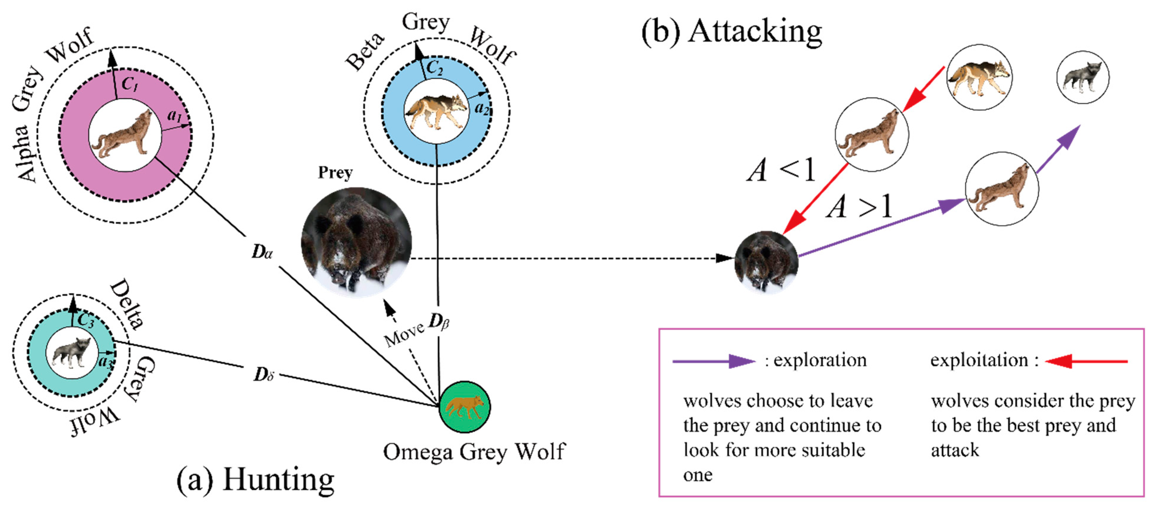
2.2. Grey Wolf Optimizer (GWO)

The grey wolf optimizer (GWO) is a meta-heuristic optimization algorithm developed by Mirjalili et al. [76], which was inspired by the predation behavior of grey wolves. GWO is characterized by a simple algorithm structure and an easy implementation, which can be applied to solve the optimization problem by adjusting the population size [77]. Nevertheless, the hunting abilities of grey wolves depend on their hierarchical social relationships. There are four classes of wolves from top to bottom in the group of grey wolves, namely alpha, beta, delta, and omega. Alpha is responsible for the development of the whole group, including hunting, resting, food distribution, etc. Beta is responsible for conveying instructions given by the alpha to other wolves and reporting to the alpha the feedback information of other wolves; who is second only to the alpha. Delta is mainly responsible for the peripheral work of the group, such as detecting prey and protecting the other wolves. If the behavior of the delta is not in the population interest, they can be demoted to the lowest class, called omega. Based on the hierarchy and division of labor in this strict social bond, the hunting behavior of grey wolves is meticulous and efficient. The detailed description was introduced in [78].

In the hunting process, the grey wolves can recognize prey by searching and tracking and surround the prey from different directions to prevent it from escape. This behavior is called encircling, which can be expressed mathematically as follows:

$$P_w(t+1)=P_p(t)-A·D D={\displaystyle |}C·P_p(t)-P_w(t){\displaystyle |}$$

(8)

where P_w and P_p represent the positions of the grey wolf and the prey, respectively. t describes the current iteration; D indicates the distance between a grey wolf and prey. A and C represent coefficients, which can be calculated by the following formula:

$$A=2a·r_1-a C=2·r_2$$

(9)

where a represents a convergence factor that decreases from 2 to 0 as the number of iterations increases. r₁ and r₂ indicate two random numbers in the range of [0, 1].

The wolves begin to move towards prey after encircling. As shown in Figure 1a, this behavior is carried out under the leadership of the alpha, with the beta and delta following the alpha to participate in the hunting occasionally. Thus, the positions of different wolves during the movement can be expressed by the following formulas:

$$D_{\alpha }=\left|C_1·P_{\alpha }(t)-P_{\omega }\right|,D_{\beta }=\left|C_2·P_{\beta }(t)-P_{\omega }\right|,D_{\delta }=\left|C_3·P_{\delta }(t)-P_{\omega }\right|$$

(10)

$$P_1=P_{\alpha }(t)-A_1·D_{\alpha },P_2=P_{\beta }(t)-A_2·D_{\beta },P_3=P_{\delta }(t)-A_3·D_{\delta },P_{\omega }(t+1)=\frac{1}{3}{P}_1+\frac{1}{3}{P}_2+\frac{1}{3}{P}_3$$

(11)

where $D_{\alpha }$, $D_{\beta }$, and $D_{\delta }$ represent the distance between the alpha ($\alpha$), beta ($\beta$), delta ($\delta$), and omega ($\omega$), respectively. P₁, P₂, and P₃ describe the current positions of the alpha ($\alpha$), beta ($\beta$), and delta ($\delta$), respectively. $P_{\omega }$ and $P_{\omega }(t+1)$ show the current and final position of the omega, respectively. Although the grey wolves have captured prey, they may give up and move on to better ones. This behavior is called exploration or exploitation (see Figure 1b) and can be controlled by A. If A > 1, the grey wolves choose to leave the prey. On the contrary, the grey wolves attack the prey.

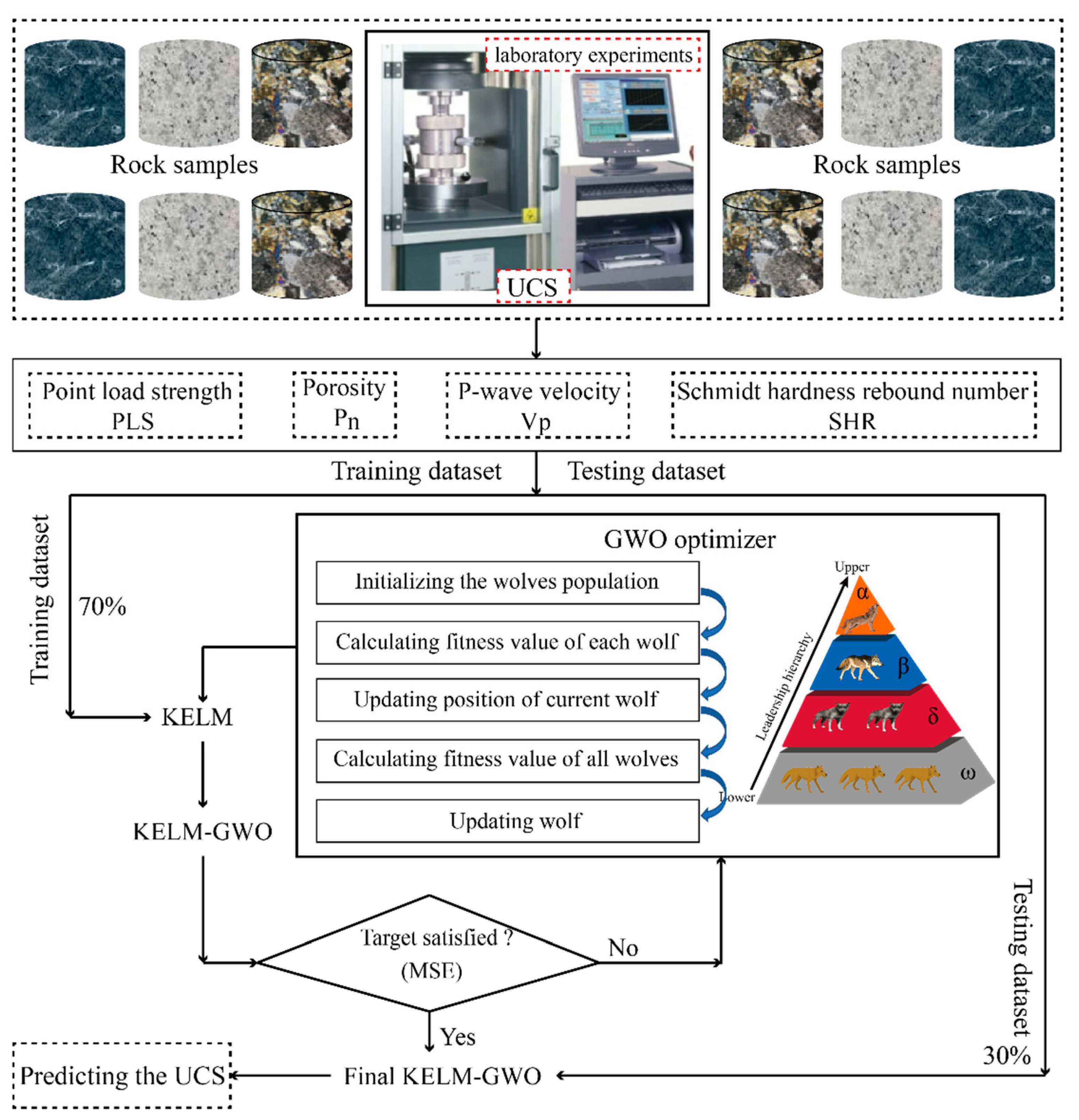
2.3. Novel Hybrid KELM-GWO

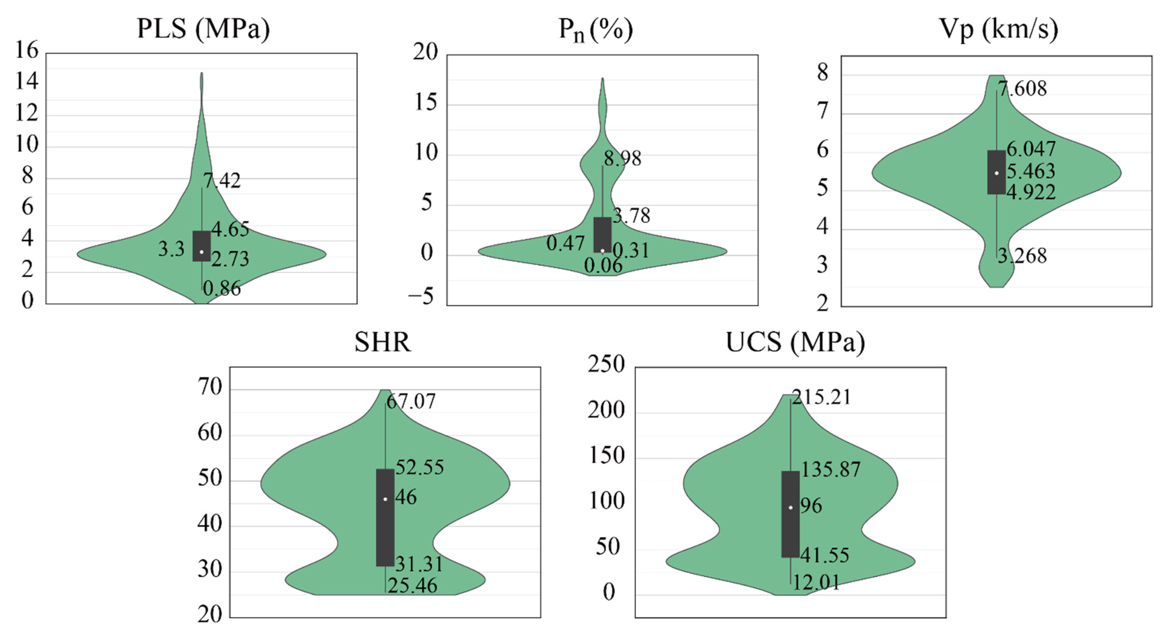
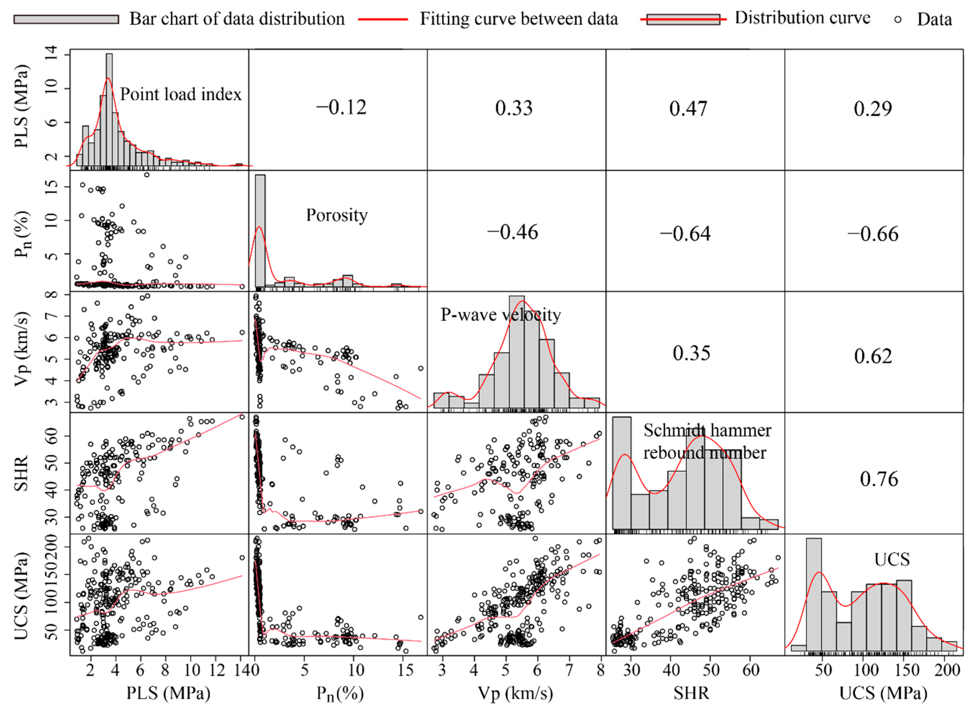
In the development of the initial KELM model, choosing the right hyperparameters combination of C and $\gamma$ had a great impact on the model performance, especially being that these parameters were not sensitive to data in the training phase [79]. Whereas, the GWO algorithm was developed to optimize similar problems by considering the number of wolves [77]. Therefore, the GWO algorithm was used to select the suitable kernel parameters (C and $\gamma$) of the KELM model for the UCS prediction in this study. To this end, 70% of the dataset was used for training the KELM-GWO model and the rest of the data (30%) was regarded as a testing set to evaluate the prediction performance of the trained model. Before running the training and testing processes, the dataset was normalized to −1 and 1 by using the MinMax scaling method. Subsequently, the initial KELM can be developed with random kernel parameters; then, the function of the GWO algorithm was to find the optimal kernel parameters that met the target prediction accuracy with different numbers of populations and iterations. The mean squared error (MSE) was applied to evaluate the predictive power of the model. In other words, the kernel parameters corresponding to the minimum value of MSE are the best for predicting UCS. The framework of the proposed KELM-GWO model to estimate UCS of rock is illustrated in Figure 2.

$$MSE=\frac{1}{n}{\displaystyle \sum _{i=1}^n{\left(y_i-y_i^{*}\right)}^2}$$

(12)

where n is the number of samples; y_i and $y_i^{*}$ are the actual and predicted values.

In order to compare the performance of UCS predicted by the KELM-GWO model and other AI models or empirical equations, such as ELM, initial KELM, DELM, BPNN, and an empirical formula were developed in this study. The principle of DELM and BPNN can found in the literature [26,48,80,81,82,83,84,85].

3. Dataset

In this study, there are 271 pieces of data of UCS obtained from various rock samples by Dehghan et al. [20], Armaghani et al. [69], and Mahmoodzadeh et al. [34], including travertine, claystone, granite, schist, sandstone, travertine, limestone, slate, etc. On the basis of previous works conducted on the UCS prediction as shown in Table 1, four parameters, namely, the porosity (P_n, %), the Schmidt hardness rebound number (SHR), the P-wave velocity (V_p, km/s), and the point load strength (PLS, MPa), were considered as input variables for the UCS (MPa) of rock samples prediction in this study. The detailed violin plots and correlation matrix of the dataset are illustrated in Figure 3 and Figure 4. The violin plots are used to show the data distributions and their probability densities. This is a type of chart which combines the features of a box chart and a density chart. The thick black bar in the middle indicates the interquartile range, while the white dot shows the median. Figure 3 clearly shows the data details of the input and output parameters, such as the minimum, minimax, and median. As can be seen in Figure 4, the relationships between their variables are nonlinear, and the three variables except P_n are positively correlated with UCS. Observing the histograms, the distributions of all variables are skewed and are bimodal skewed distributions. Accordingly, all variables need to be normalized before being applied to the models.

4. Performance Indices for the Assessment of Models

In this study, the root mean square error (RMSE), the determination coefficient (R²), the mean absolute error (MAE), the prediction accuracy (U₁), the prediction quality (U₂), and the variance accounted for (VAF) were used as performance indicators to evaluate the reliability and accuracy of all AI models and empirical formula for predicting UCS. These indicators are defined as follows [47,49,86,87,88,89,90,91,92,93,94,95]:

$$\mathrm{RMSE}=\sqrt{\frac{1}{n}{\displaystyle \sum _{i=1}^n{\left(UC{S}_{o,i}-UC{S}_{p,i}\right)}^2}}$$

(13)

$${\mathrm{R}}^2=1-\frac{{\left[{\displaystyle \sum _{i=1}^n(UC{S}_{o,i}-UC{S}_{p,i})}\right]}^2}{{\left[{\displaystyle \sum _{i=1}^n(UC{S}_{o,i}-\overline{UC{S}_o})}\right]}^2}$$

(14)

$$\mathrm{MAE}=\frac{1}{n}{\displaystyle \sum _{i=1}^n{\displaystyle |}UC{S}_{o,i}-UC{S}_{p,i}{\displaystyle |}}$$

(15)

$${\mathrm{U}}_1=\frac{RMSE}{\sqrt{\frac{1}{n}{\displaystyle {\sum }_{i=1}^{n}UC{S}_{o,i}{}^2}}+\sqrt{\frac{1}{n}{\displaystyle {\sum }_{i=1}^{n}UC{S}_{p,i}{}^2}}}$$

(16)

$${\mathrm{U}}_2=\frac{{\displaystyle {\sum }_{i=1}^n{(UC{S}_{o,i}-UC{S}_{p,i})}^2}}{{\displaystyle {\sum }_{i=1}^{n}UC{S}_{o,i}{}^2}}$$

(17)

$$\mathrm{VAF}=\left[1-\frac{\mathrm{var}(UC{S}_{o,i}-UC{S}_{p,i})}{\mathrm{var}(UC{S}_{o,i})}\right]\times 100$$

(18)

where n represents the number of rock samples in the training or testing phase, $UC{S}_{o,i}$ and $\overline{UC{S}_o}$ are the observed values and mean observed values of UCS, respectively, $UC{S}_{p,i}$ and $\overline{UC{S}_p}$ are predicted values and mean predicted values of UCS, respectively.

5. Developing the Models for Predicting UCS

In this study, five AI models (i.e., ELM, KELM, KELM-GWO, DELM, and BPNN) and one empirical model have been developed to predict UCS of rock samples. In what follows, the development of the models is presented and discussed comprehensively.

5.1. ELM

To develop a suitable ELM model for UCS prediction, an SLFN architecture should initially be created with a certain number of neurons in a single hidden layer. For this purpose, the number of neurons was set in the range of 20–150 and 14 ELM models were proposed in this study. RMSE and R² were used to select the optimal number of hidden layer neurons, which means that the number of neurons corresponding to the model with the lowest value of RMSE and the highest values of R² is the best model for predicting the UCS. As can be seen in

Table 2. Performance evaluation of ELM models with different number of neurons in the hidden layer.

Model No.	Neurons of Hidden Layer	RMSE		R2
		Training	Testing	Training	Testing
1	20	28.7283	27.4770	0.6786	0.7050
2	30	24.0466	21.9013	0.7480	0.8126
3	40	22.5454	21.5436	0.8021	0.8186
4	50	22.1986	21.7206	0.8081	0.8157
5	60	22.3844	21.3123	0.8049	0.8225
6	70	19.6458	22.7176	0.8497	0.7983
7	80	19.9072	25.3655	0.8457	0.7486
8	90	17.6883	31.2900	0.8782	0.7683
9	100	18.7275	25.3018	0.8634	0.7499
10	110	17.5671	23.6957	0.8798	0.7806
11	120	18.8266	27.1939	0.8620	0.7110
12	130	18.6357	34.9914	0.8648	0.5216
13	140	16.8519	34.6346	0.8894	0.5313
14	150	17.1542	34.7546	0.8714	0.5285

Note: Line in bold represents the better solution.

, in model number 5 with 60 neurons in the hidden layer, the lowest RMSE and the highest R² were obtained in the testing phase, even if it was not optimal in the training phase. Therefore, an SLFN architecture with 60 neurons in the hidden layer was considered for the ELM model to predict UCS in the following study.

5.2. KELM

The KELM model is an improved version of the ELM model to predict UCS by using kernel functions. Therefore, the numbers of neurons in the hidden layer no longer need to be changed, but different kernel parameters were chosen to predict UCS. In particular, the values range of the kernel parameters should depend on the specific problem, such as the range of [2⁻²⁰, 2²⁰] being used by Zhu et al. [79] and the range of [2⁻⁸, 2⁸] being considered by Baliarsingh et al. [96]. To determine these parameters, the C and $\gamma$ were the same and changed in the range [2⁻², 2⁹]. The performance of the KELM models with different kernel parameters was evaluated in terms of RMSE and R² in the training and testing phase, as shown in Figure 5. As can be seen in this figure, the KELM model with the lowest RMSE and the highest R² is considered as the best model, which has the best kernel parameters of C and $\gamma$ being 2⁰.

5.3. KELM-GWO

Although the KELM model with the kernel parameters C and $\gamma$ of 2⁰ show a good predictive performance, it is not practical to manually test every possible parameter combination due to the large range of [2⁻², 2⁹]. Therefore, the modified KELM with the new kernel parameters was obtained by using the GWO algorithm, and a reasonable comparison between the KELM and novel hybrid KELM-GWO could be conducted. It is interesting to note that only the numbers of grey wolves should be tuned in the GWO algorithm to optimize the other models [77]. To this purpose, the populations of grey wolves were considered to be equal to 25, 50, 75, 100, 150, and 200 for 600 iterations in this study. Meanwhile, the MSE is used as the stopping condition to select the optimal population, as shown in Figure 6. As can be seen in this figure, the numbers of populations have no effect on the fitness values after 500 iterations. The ideal KELM-GWO model with the lowest MSE was reached at the population of 75, where it has the best kernel parameters of C = 254.63 and $\gamma$ = 0.52, respectively. Therefore, the final KELM-GWO model considering C = 254.63 and $\gamma$ = 0.52 was used for predicting UCS of rock samples.

5.4. DELM

Similar to other neural network models, the performance of the DELM model is also controlled by the numbers of hidden layers and the corresponding number of neurons. For this purpose, 3, 4, and 5 multi-hidden layers with different numbers of neurons (5, 10, and 15) were considered to predict UCS. To verify the performance of all DELM models, the RMSE and R² were also recorded in the training and testing phases, as shown in

Table 3. Performance evaluation of DELM models with various numbers of hidden layers.

Model Multi-Hidden Layers	RMSE		R2
	Training	Testing	Training	Testing
5-5-5	31.1924	30.0702	0.6211	0.6467
10-10-10	28.4753	27.6212	0.6843	0.7019
15-15-15	28.5459	27.6791	0.6827	0.7006
5-5-5-5	34.0340	32.3176	0.5490	0.5919
10-10-10-10	35.5967	33.8719	0.5066	0.5517
15-15-15-15	32.3059	30.5482	0.5936	0.6354
5-5-5-5-5	32.1756	30.6333	0.5969	0.6333
10-10-10-10-10	34.0784	33.2670	0.5478	0.5676
15-15-15-15-15	40.7977	39.3185	0.3519	0.3959

Note: Line in bold represents the better solution.

. As can be seen in this table, in the DELM model with numbers of 10-10-10 neurons in three hidden layers, the lowest value of RMSE and the highest value of R² in the training and testing phase were obtained and recorded, respectively. Therefore, the DELM model considering the numbers of 10-10-10 neurons in three hidden layers was selected to predict UCS in this study, as illustrated in Figure 7.

5.5. BPNN

BPNN is a typically and widely used neural network model for prediction problems in geotechnical engineering [80,81]. To develop an effective BPNN model for predicting UCS of rock samples, the numbers of hidden layers and neurons should be determined to prevent overfitting and reduce the computation time. Therefore, double hidden layers with different neurons were developed; the RMSE and R² were recorded as evaluation indicators to compare the performance of all models.

Table 4. Performance evaluation of BPNN with various neurons of two hidden layers.

Model	Hidden Layers		RMSE		R2
	1	2	Training	Testing	Training	Testing
1	2	2	24.7580	20.6986	0.7613	0.8326
2	2	4	20.3518	17.7909	0.8387	0.8763
3	2	6	21.6890	24.4836	0.8168	0.7658
4	2	8	20.0367	17.5967	0.8437	0.8790
5	2	10	25.3568	21.7866	0.7496	0.8145
6	4	4	20.4635	18.0377	0.8369	0.8729
7	4	6	23.7747	21.6982	0.7799	0.8160
8	4	8	19.9445	17.2805	0.8602	0.8833
9	4	10	20.0098	17.9689	0.8441	0.8738
10	6	6	24.7290	20.3359	0.7619	0.8384
11	6	8	19.2109	17.1627	0.8563	0.8849
12	6	10	22.4402	18.1689	0.8039	0.8710
13	8	8	19.7370	17.5722	0.8633	0.8793
14	8	10	22.5188	19.8386	0.8025	0.8462
15	10	10	22.7941	19.1961	0.7941	0.8560

Note: Line in bold represents the better solution.

shows a summary of the obtained values of RMSE and R² in the training and testing phases. As can be seen in this table, model number 11, i.e., two hidden layers with 6 and 8 neurons, has shown the lowest value of RMSE in both the training and testing phases; the highest value of R² in the testing phase. Therefore, model number 11 was considered as the final BPNN model to predict UCS, as depicted in Figure 8.

5.6. Empirical Model

Multivariate regression analysis (MRA) is a useful tool to create an empirical model for predicting UCS, as summarized in Table 1. MRA is made of various parameters to achieve the best-fit equation through performing the least squares fit, which can be described as a multivariate equation of first order by Armaghani et al. [97]. Therefore, an empirical formula, Equation (19), was proposed to predict UCS based on the four input variables considered in this study.

$$UCS=-128.37-3.34\times \mathrm{PLS}-0.776\times {\mathrm{P}}_{\mathrm{n}}+0.0212\times {\mathrm{V}}_{\mathrm{p}}+2.789\times \mathrm{SHR}$$

(19)

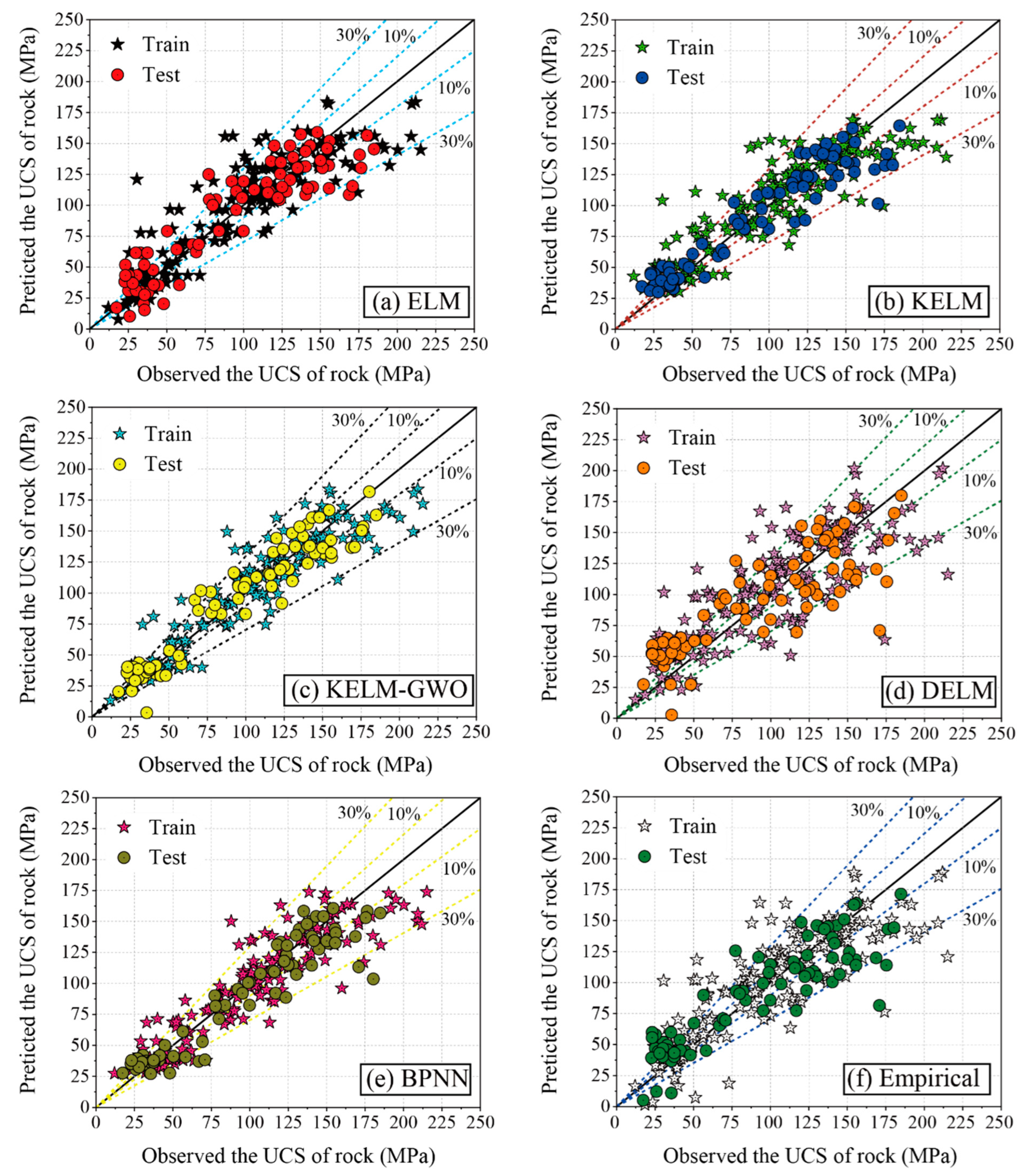
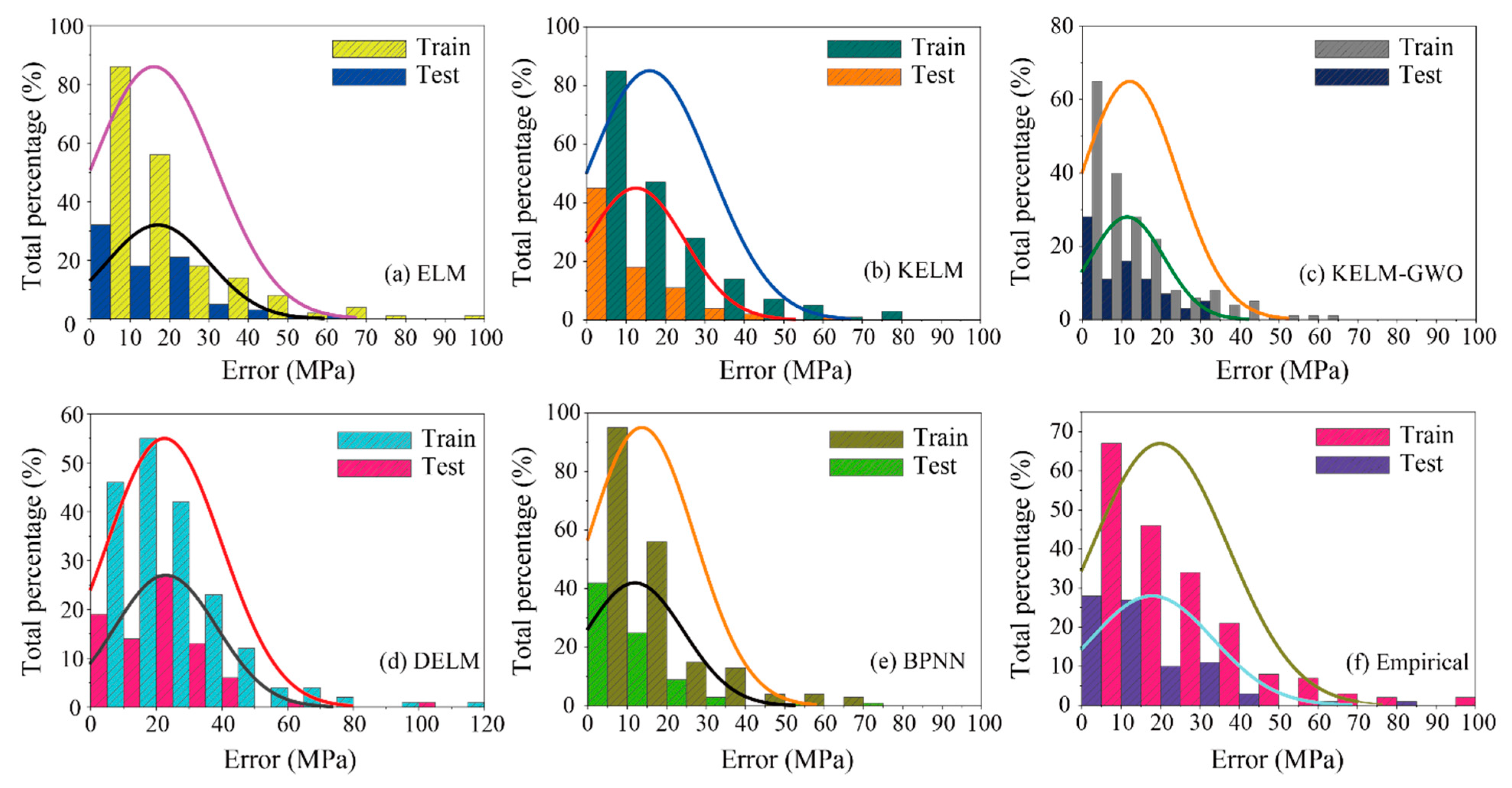
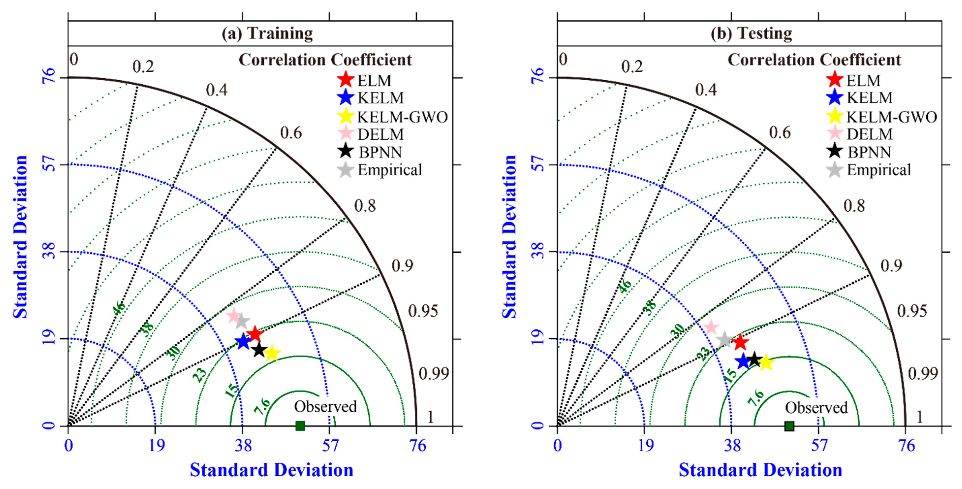
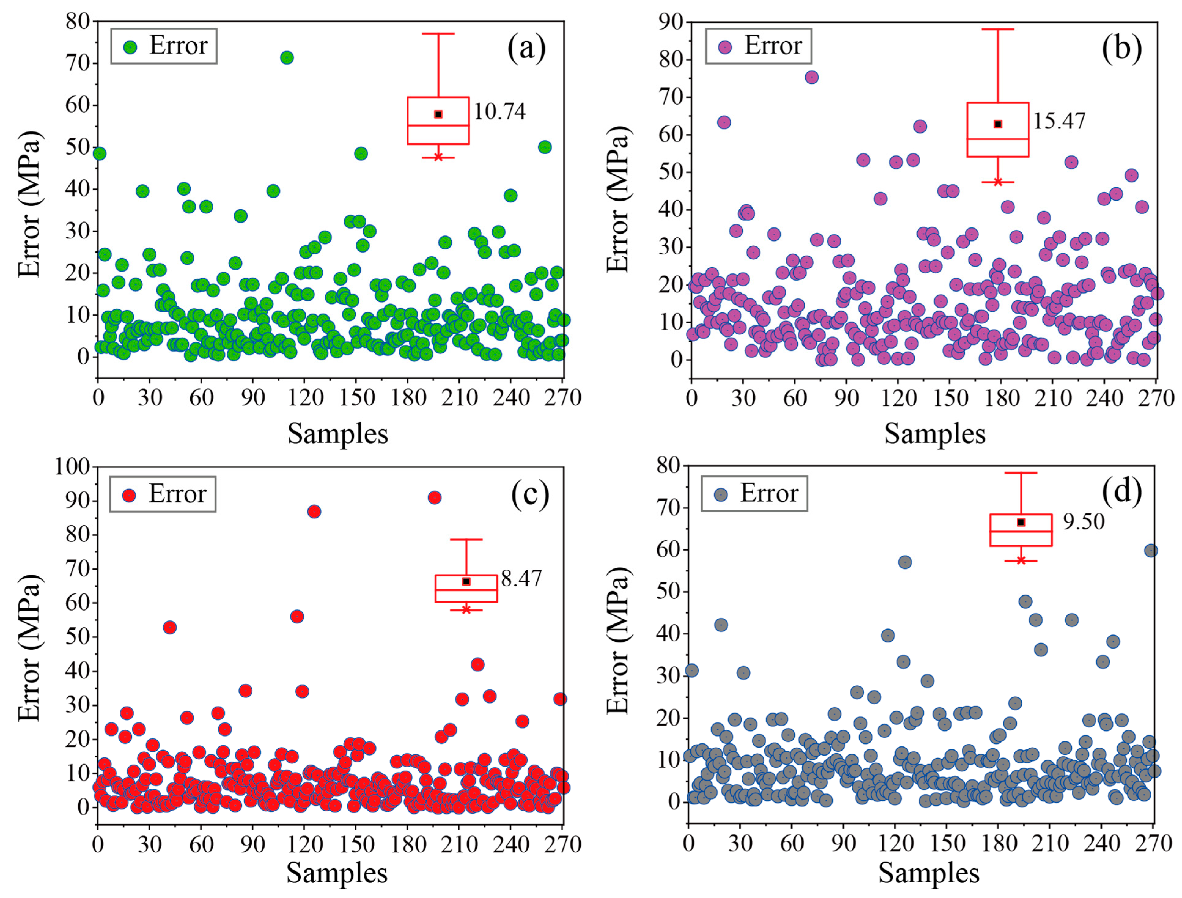
6. Results and Discussion

The ELM, KELM, KELM-GWO, DELM, BPNN models, and the empirical equation were run to predict UCS after ensuring that the optimal involving parameters and the performance of all the six models were evaluated in terms of six statistical indices (i.e., RMSE, R², MAE, U₁, U₂, and VAF) previously mentioned in this study. The results of the performance indices in the training and testing phases of all models were represented in

Table 5. Comparison of the performances of all models (training phase).

Model	Performance (Training)
	RMSE	R2	MAE	U1	U2	VAF (%)
ELM	22.3844	0.8049	15.9951	0.1041	0.0443	80.4891
KELM	22.2684	0.8069	15.9380	0.1038	0.0442	80.7237
KELM-GWO	17.2176	0.8846	12.0577	0.0798	0.0259	88.4566
DELM	28.4753	0.6843	22.4743	0.1306	0.0677	69.1651
BPNN	19.2109	0.8563	13.6784	0.0905	0.0344	85.9230
Empirical	26.3309	0.7300	19.8876	0.1223	0.0610	73.0331
Model	Performance (Testing)
	RMSE	R2	MAE	U1	U2	VAF (%)
ELM	21.3123	0.8225	17.0308	0.1038	0.0452	82.4108
KELM	17.5050	0.8803	12.4699	0.0854	0.0308	88.1894
KELM-GWO	14.7327	0.9152	11.4315	0.0706	0.0259	91.5207
DELM	27.6213	0.7019	22.9152	0.1332	0.0730	70.3401
BPNN	17.1627	0.8849	11.9449	0.0945	0.0305	89.4529
Empirical	24.0864	0.7733	18.2310	0.1181	0.0595	77.6171

Note: Line in bold represents the better solution.

. As can be seen in this table, the KELM-GWO model was the best model for predicting UCS with the best performance indices in both the training (RMSE: 17.2176; R²: 0.8846; MAE: 12.0577; U₁: 0.0798; U₂: 0.0259; VAF: 88.4566%) and testing phases (RMSE: 14.2176; R²: 0.9152; MAE: 11.4315; U₁: 0.0706; U₂: 0.0259; VAF: 91.5207%). Nevertheless, it is important to note that not all AI models perform better than the empirical formulas. It should be noted that the DELM model is worse than the empirical formula in both training and testing phases with an RMSE of 28.4753–27.6213, R² of 0.6843–0.7019, MAE of 22.4743–22.9152, U₁ of 0.1306–0.1332, U₂ of 0.0677–0.0730, and VAF of 69.1654–70.3401%. The reason for this result is that the DELM lacks a reverse fine-tuning process compared with a traditional deep learning algorithm. Although more hidden layers are added, excessive input weights aggravate the training load and result in a low prediction performance. After the KELM-GWO model, the BPNN, KELM, and ELM have a close competition in both the training and testing phases.

To further compare the predictive performance of the six models, the regression diagrams of all the models in the training and testing phases are demonstrated in Figure 9. As can be seen in this figure, the horizontal and vertical axes represent the observed values of UCS measured in laboratory experiments and the predicted values proposed by AI models and the empirical equation in this study, respectively. Particularly, the data point will appear on the black diagonal line in each diagram when the predicted value is equal to the observed value. Meanwhile, other radial lines with 10% and 30% are second and third criteria to indicate deviations from the predicted values. Accordingly, the more predicted values appear within the 10% and 30% lines and the closer they are to the black diagonal line, the better the prediction performance of the model. As can be realized, the KELM-GWO model not only has the least predicted values outside the 30% line, but also has the most predicted values close to the black diagonal line in both the training and testing phases. After the KELM-GWO model, BPNN, KELM, and ELM have a similar prediction performance. Nevertheless, there are more predicted values of UCS away from the black diagonal in the empirical and DELM model.

To clearly show the performance of the six models in the training and testing phases, the error histograms were described in Figure 10. The horizontal axis and the vertical axis represent the error between the predicted value and its total percentage (%), respectively. That is to say, increasing the tall error bars close to the origin, increases the prediction accuracy of the model. As can be seen in this figure, the percentage of the lowest error is highest in the KELM-GWO model and the lowest in the DELM model.

Figure 11 shows the error curves of the six models in the testing phase. There are two types of curves in each diagram: the black curve represents observed values, and the other colored curves represent predicted values for each model. Taken as a whole, the predictive performance of each model in the testing phase is close. Nevertheless, magnified local errors can indicate differences in the predictive performance of all the models. As can be seen in these diagrams, there are smaller predicted errors from rock samples of No. 65 to No. 81 in the KELM-GWO model than the other five models, which means that the KELM-GWO model is more suitable for predicting UCS than other models.

The graphical Taylor diagrams can be a concise tool for evaluating the performance of the models more comprehensively, as shown in Figure 12. A complete Taylor diagram consists of three parts: standard deviation (blue circles), RMSE (green circles), and correlation coefficient (black dotted lines). The RMSE and correlation coefficient of the observed value was 0 and 1; the standard deviation, RMSE, and correlation coefficient of all models can be calculated based on their predicted values. Accordingly, the highest similarity to the observed data corresponded to the best prediction model. As can be seen in the diagrams, the KELM-GWO model was the best model with the closest position to the observed values in both the training and testing phases. After this model, the ranking of the prediction performance is BPNN, KELM, ELM, empirical, and DELM.

To compare and assess the prediction performance with the proposed model, the current and previous works are listed in

Table 6. Comparison between the current and previous works by using AI algorithms for UCS of rock prediction.

References	AI Models	Input Parameters	No. of Dataset	Performance
[20]	ANN	PLS, Vp, SHR, Pn	30	R2 = 0.93
[21]	GP	Pn, r, Vp	72	RMSE = 12.3
[24]	ANN	r, CC, QC	138	R2 = 0.76
[25]	ANN	Pn, SD, SH, PLS	39	R2 = 0.93
[28]	FIS	SDI2, SDI4, CLC	65	RMSE = 2.767
[29]	FIS	BPI, PLS, SHR, Vp, Pn, r	60	R2 = 0.98 RMSE = 8.21
[30]	FIS	SH, r, Pn	75	R2 = 0.9437
[31]	SVM	Pn, Vp, SD	47	R2 = 0.7712
[32]	SVM	Vp, Pn, SHR	85	R2 = 0.9516 RMSE = 2.14
[33]	SVM	Vp, SHR, CSS	90	R2 = 0.867
[34]	SVM	SH, Pn, Vp, PLS	170	R2 = 0.9363 RMSE = 1.097
[35]	RF	PLS, Pn, Vp, SHR	30	R2 = 0.93
[36]	RF	Vp, SH, Pn, PLS	93	R2 = 0.488 RMSE = 8.071
[40]	MLP	RC, r, Pn, Vp, WA, PLS	197	R2 = 0.90 RMSE = 0.289
[41]	GEP	UPV, WA, Dd, Sd, Bd	167	R2 = 0.877
[43]	GA	QC, r, Pn, CI, SSH	44	R2 = 0.63
[101]	ANN	WS, r, Pn	83	R2 = 0.96
[102]	ANN	Vp, r, Pn	105	R2 = 0.95
This study	ELM KELM KELM-GWO DELM BPNN	SH, Pn, Vp, PLS	271	R2ELM = 0.8225 R2KELM = 0.8803 R2KELM-GWO = 0.9152 R2DELM = 0.7019 R2BPNN = 0.8849

Note: QC: quartz content; SH: shore hardness; SHR: Schmidt hardness rebound number; CI: cone indenter hardness; CC: concavity/convexity; SD: slake durability; SDI: slake durability index; SDI₂: two-cycle slake durability index; SDI₄: four-cycle slake durability index; CLC: clay content; CSS: cubic sample sizes; RC: rock class; WA: water absorption; WS: water saturation; UPV: ultrasound pulse velocity; Dd: dry density; Sd: saturated density; Bd: bulk density; SSH: shore scleroscope hardness; GWO: grey wolf optimizer.

. As can be seen in this table, the KELM model was almost never used to predict UCS and the KELM-GWO model proposed in this study is better than most of the single AI models. Although the performance results of several studies are better than this paper, the volume of data limits the difficulty of applying these models to the UCS prediction of other rocks. In addition, different prediction results can be obtained by using different input parameter combinations based on the same model. Therefore, it is necessary to obtain the importance of the different input parameters for the UCS prediction in this study.

The mean impact value (MIV) has been reported to analyze the importance of input variables in prediction problems [98,99,100]. The core of the MIV technique is enlarging and reducing the input variable with the same ratio. Then, two new kinds of datasets were used to train and test based on the proposed models. Accordingly, two new outputs were obtained and the errors between them were named as impact values (IVs) of the input variable. Finally, the mean of those IVs (MIV) can be calculated and the largest MIV of the variable represents the highest importance for predicting UCS. The results of importance analysis for input variables are illustrated in Figure 13. As can be seen in this figure, the most important input variable is n with an MIV of 15.47; the remaining order of importance for the others is PLS of 10.74, SHR of 9.50, and V_p of 8.47.

7. Conclusions and Summary

The UCS is a parameter of great importance for designing geotechnical and mining works such as tunneling, underground excavation, rock slope stability, and dam construction. Therefore, five AI models (ELM, KELM, KELM-GWO, DELM, and BPNN) and an empirical equation were proposed to predict UCS based on the 271 rock samples. The results showed that the KELM-GWO model was the best model for predicting UCS with the best performance indices in both the training (RMSE: 17.2176; R²: 0.8846; MAE: 12.0577; U₁: 0.0798; U₂: 0.0259; VAF: 88.4566%) and testing phases (RMSE: 14.2176; R²: 0.9152; MAE: 11.4315; U₁: 0.0706; U₂: 0.0259; VAF: 91.5207%). It is also verified that GWO is an effective algorithm to improve the prediction performance of the KELM model. The porosity is the most important parameter for predicting UCS by using the MIV technique; the remaining order of importance for the others is point load strength of 10.74, Schmidt hardness rebound number of 9.50, and P-wave velocity of 8.47. This paper highlights the performance advantages of hybrid algorithms and the use of integrated large databases, but the parameter diversity considered in this paper limits the prediction performance to a certain extent. We believe that on the premise of fusing more reference data, increasing effective input parameters as much as possible is helpful to improve the predictive performance of the hybrid model.

References

1. Bieniawski, Z.T. Estimating the strength of rock materials. J. S. Afr. Inst. Min. Metall. 1974, 74, 312–320. [Google Scholar] [CrossRef]
2. Gokceoglu, C.; Zorlu, K. A fuzzy model to predict the uniaxial compressive strength and the modulus of elasticity of a problematic rock. Eng. Appl. Artif. Intell. 2004, 17, 61–72. [Google Scholar] [CrossRef]
3. Luo, Y. Influence of water on mechanical behavior of surrounding rock in hard-rock tunnels: An experimental simulation. Eng. Geol. 2020, 277, 105816. [Google Scholar]
4. Elmo, D.; Donati, D.; Stead, D. Challenges in the characterisation of intact rock bridges in rock slopes. Eng. Geol. 2018, 245, 81–96. [Google Scholar] [CrossRef]
5. Ghasemi, E.; Kalhori, H.; Bagherpour, R.; Yagiz, S. Model tree approach for predicting uniaxial compressive strength and Young’s modulus of carbonate rocks. Bull. Eng. Geol. Environ. 2018, 77, 331–343. [Google Scholar]
6. Mahmoodzadeh, A.; Mohammadi, M.; Daraei, A.; Faraj, R.H.; Omer, R.; Sherwani, A.F.H. Decision-making in tunneling using artificial intelligence tools. Tunn. Undergr. Space Technol. 2020, 103, 103514. [Google Scholar] [CrossRef]
7. Armaghani, D.J.; Safari, V.; Fahimifar, A.; Amin, M.F.M.; Monjezi, M.; Mohammadi, M.A. Uniaxial compressive strength prediction through a new technique based on gene expression programming. Neural Comput. Appl. 2018, 30, 3523–3532. [Google Scholar] [CrossRef]
8. Ying, J.; Han, Z.; Shen, L.; Li, W. Influence of Parent Concrete Properties on Compressive Strength and Chloride Diffusion Coefficient of Concrete with Strengthened Recycled Aggregates. Materials 2020, 13, 4631. [Google Scholar] [CrossRef] [PubMed]
9. Parsajoo, M.; Armaghani, D.J.; Mohammed, A.S.; Khari, M.; Jahandari, S. Tensile strength prediction of rock material using non-destructive tests: A comparative intelligent study. Transp. Geotech. 2021, 31, 100652. [Google Scholar] [CrossRef]
10. Koopialipoor, M.; Asteris, P.G.; Mohammed, A.S.; Alexakis, D.E.; Mamou, A.; Armaghani, D.J. Introducing stacking machine learning approaches for the prediction of rock deformation. Transp. Geotech. 2022, 34, 100756. [Google Scholar]
11. Kahraman, S. Evaluation of simple methods for assessing the uniaxial compressive strength of rock. Int. J. Rock Mech. Min. Sci. 2001, 38, 981–994. [Google Scholar] [CrossRef]
12. Mahdiabadi, N.; Khanlari, G. Prediction of Uniaxial Compressive Strength and Modulus of Elasticity in Calcareous Mudstones Using Neural Networks, Fuzzy Systems, and Regression Analysis. Period. Polytech. Civ. Eng. 2019, 63, 104–114. [Google Scholar] [CrossRef]
13. Baykasoğlu, A.; Güllü, H.; Canakci, H.; Özbakır, L. Prediction of compressive and tensile strength of limestone via genetic programming. Expert Syst. Appl. 2008, 35, 111–123. [Google Scholar] [CrossRef]
14. Yılmaz, I.; Sendır, H. Correlation of Schmidt hardness with unconfined compressive strength and Young’s modulus in gypsum from Sivas (Turkey). Eng. Geol. 2002, 66, 211–219. [Google Scholar] [CrossRef]
15. obanoğlu, İ.; Çelik, S.B. Estimation of uniaxial compressive strength from point load strength, Schmidt hardness and P-wave velocity. Bull. Eng. Geol. Environ. 2008, 67, 491–498. [Google Scholar] [CrossRef]
16. Sharma, P.K.; Singh, T.N. A correlation between P-wave velocity, impact strength index, slake durability index and uniaxial compressive strength. Bull. Eng. Geol. Environ. 2008, 67, 17–22. [Google Scholar] [CrossRef]
17. Khandelwal, M.; Singh, T. Correlating static properties of coal measures rocks with P-wave velocity. Int. J. Coal Geol. 2009, 79, 55–60. [Google Scholar] [CrossRef]
18. Kahraman, S. The determination of uniaxial compressive strength from point load strength for pyroclastic rocks. Eng. Geol. 2014, 170, 33–42. [Google Scholar] [CrossRef]
19. Mohamad, E.T.; Armaghani, D.J.; Momeni, E.; Abad, S.V.A.N.K. Prediction of the unconfined compressive strength of soft rocks: A PSO-based ANN approach. Bull. Eng. Geol. Environ. 2015, 74, 745–757. [Google Scholar] [CrossRef]
20. Dehghan, S.; Sattari, G.; Chelgani, S.C.; Aliabadi, M. Prediction of uniaxial compressive strength and modulus of elasticity for Travertine samples using regression and artificial neural networks. Min. Sci. Technol. 2010, 20, 41–46. [Google Scholar] [CrossRef]
21. Beiki, M.; Majdi, A.; Givshad, A.D. Application of genetic programming to predict the uniaxial compressive strength and elastic modulus of carbonate rocks. Int. J. Rock Mech. Min. Sci. 2013, 63, 159–169. [Google Scholar] [CrossRef]
22. Grima, M.A.; Babuška, R. Fuzzy model for the prediction of unconfined compressive strength of rock samples. Int. J. Rock Mech. Min. Sci. 1999, 36, 339–349. [Google Scholar] [CrossRef]
23. Tiryaki, B. Predicting intact rock strength for mechanical excavation using multivariate statistics, artificial neural networks, and regression trees. Eng. Geol. 2008, 99, 51–60. [Google Scholar] [CrossRef]
24. Zorlu, K.; Gokceoglu, C.; Ocakoglu, F.; Nefeslioglu, H.; Acikalin, S. Prediction of uniaxial compressive strength of sandstones using petrography-based models. Eng. Geol. 2008, 96, 141–158. [Google Scholar] [CrossRef]
25. Yılmaz, I.; Yuksek, A.G. An Example of Artificial Neural Network (ANN) Application for Indirect Estimation of Rock Parameters. Rock Mech. Rock Eng. 2008, 41, 781–795. [Google Scholar]
26. Sarkar, K.; Tiwary, A.; Singh, T.N. Estimation of strength parameters of rock using artificial neural networks. Bull. Eng. Geol. Environ. 2010, 69, 599–606. [Google Scholar] [CrossRef]
27. Sonmez, H.; Tuncay, E.; Gokceoglu, C. Models to predict the uniaxial compressive strength and the modulus of elasticity for Ankara Agglomerate. Int. J. Rock Mech. Min. Sci. 2004, 41, 717–729. [Google Scholar] [CrossRef]
28. Gokceoglu, C.; Sonmez, H.; Zorlu, K. Estimating the uniaxial compressive strength of some clay-bearing rocks selected from Turkey by nonlinear multivariable regression and rule-based fuzzy models. Expert Syst. 2009, 26, 176–190. [Google Scholar] [CrossRef]
29. Mishra, D.; Basu, A. Estimation of uniaxial compressive strength of rock materials by index tests using regression analysis and fuzzy inference system. Eng. Geol. 2013, 160, 54–68. [Google Scholar]
30. Rezaei, M.; Majdi, A.; Monjezi, M. An intelligent approach to predict unconfined compressive strength of rock surrounding access tunnels in longwall coal mining. Neural Comput. Appl. 2014, 24, 233–241. [Google Scholar] [CrossRef]
31. Ceryan, N. Application of support vector machines and relevance vector machines in predicting uniaxial compressive strength of volcanic rocks. J. Afr. Earth Sci. 2014, 100, 634–644. [Google Scholar]
32. Barzegar, R.; Sattarpour, M.; Nikudel, M.R.; Moghaddam, A.A. Comparative evaluation of artificial intelligence models for prediction of uniaxial compressive strength of travertine rocks, Case study: Azarshahr area, NW Iran. Model. Earth Syst. Environ. 2016, 2, 76. [Google Scholar] [CrossRef]
33. Çelik, S.B. Prediction of uniaxial compressive strength of carbonate rocks from nondestructive tests using multivariate regression and LS-SVM methods. Arab. J. Geosci. 2019, 12, 193. [Google Scholar]
34. Mahmoodzadeh, A.; Mohammadi, M.; Ibrahim, H.H.; Abdulhamid, S.N.; Salim, S.G.; Ali, H.F.H.; Majeed, M.K. Artificial intelligence forecasting models of uniaxial compressive strength. Transp. Geotech. 2021, 27, 100499. [Google Scholar]
35. Matin, S.; Farahzadi, L.; Makaremi, S.; Chelgani, S.C.; Sattari, G. Variable selection and prediction of uniaxial compressive strength and modulus of elasticity by random forest. Appl. Soft Comput. 2018, 70, 980–987. [Google Scholar] [CrossRef]
36. Barzegar, R.; Sattarpour, M.; Deo, R.; Fijani, E.; Adamowski, J. An ensemble tree-based machine learning model for predicting the uniaxial compressive strength of travertine rocks. Neural Comput. Appl. 2020, 32, 9065–9080. [Google Scholar]
37. Yilmaz, I.; Yuksek, G. Prediction of the strength and elasticity modulus of gypsum using multiple regression, ANN, and ANFIS models. Int. J. Rock Mech. Min. Sci. 2009, 46, 803–810. [Google Scholar] [CrossRef]
38. Yesiloglu-Gultekin, N.; Sezer, E.A.; Gokceoglu, C.; Bayhan, H. An application of adaptive neuro fuzzy inference system for estimating the uniaxial compressive strength of certain granitic rocks from their mineral contents. Expert Syst. Appl. 2013, 40, 921–928. [Google Scholar] [CrossRef]
39. Chentout, M.; Alloul, B.; Rezouk, A.; Belhai, D. Experimental study to evaluate the effect of travertine structure on the physical and mechanical properties of the material. Arab. J. Geosci. 2015, 8, 8975–8985. [Google Scholar] [CrossRef]
40. Asheghi, R.; Shahri, A.A.; Zak, M.K. Prediction of Uniaxial Compressive Strength of Different Quarried Rocks Using Metaheuristic Algorithm. Arab. J. Sci. Eng. 2019, 44, 8645–8659. [Google Scholar]
41. Çanakcı, H.; Baykasoğlu, A.; Güllü, H. Prediction of compressive and tensile strength of Gaziantep basalts via neural networks and gene expression programming. Neural Comput. Appl. 2009, 18, 1031–1041. [Google Scholar] [CrossRef]
42. Ozbek, A.; Unsal, M.; Dikec, A. Estimating uniaxial compressive strength of rocks using genetic expression programming. J. Rock Mech. Geotech. Eng. 2013, 5, 325–329. [Google Scholar] [CrossRef]
43. Manouchehrian, A.; Sharifzadeh, M.; Moghadam, R.H.; Nouri, T. Selection of regression models for predicting strength and deformability properties of rocks using GA. Int. J. Min. Sci. Technol. 2013, 23, 495–501. [Google Scholar] [CrossRef]
44. Liu, Z.; Shao, J.; Xu, W.; Wu, Q. Indirect estimation of unconfined compressive strength of carbonate rocks using extreme learning machine. Acta Geotech. 2015, 10, 651–663. [Google Scholar] [CrossRef]
45. Zeng, J.; Roy, B.; Kumar, D.; Mohammed, A.S.; Armaghani, D.J.; Zhou, J.; Mohamad, E.T. Proposing several hybrid PSO-extreme learning machine techniques to predict TBM performance. Eng. Comput. 2021, 1–17. [Google Scholar] [CrossRef]
46. Lu, X.; Hasanipanah, M.; Brindhadevi, K.; Amnieh, H.B.; Khalafi, S. ORELM: A Novel Machine Learning Approach for Prediction of Flyrock in Mine Blasting. Nonrenew. Resour. 2020, 29, 641–654. [Google Scholar] [CrossRef]
47. Murlidhar, B.R.; Kumar, D.; Armaghani, D.J.; Mohamad, E.T.; Roy, B.; Pham, B.T. A Novel Intelligent ELM-BBO Technique for Predicting Distance of Mine Blasting-Induced Flyrock. Nonrenew. Resour. 2020, 29, 4103–4120. [Google Scholar] [CrossRef]
48. Li, C.; Zhou, J.; Khandelwal, M.; Zhang, X.; Monjezi, M.; Qiu, Y. Six Novel Hybrid Extreme Learning Machine–Swarm Intelligence Optimization (ELM–SIO) Models for Predicting Backbreak in Open-Pit Blasting. Nonrenew. Resour. 2022, 1–23. [Google Scholar] [CrossRef]
49. Armaghani, D.J.; Kumar, D.; Samui, P.; Hasanipanah, M.; Roy, B. A novel approach for forecasting of ground vibrations resulting from blasting: Modified particle swarm optimization coupled extreme learning machine. Eng. Comput. 2021, 37, 3221–3235. [Google Scholar] [CrossRef]
50. Bardhan, A.; Kardani, N.; GuhaRay, A.; Burman, A.; Samui, P.; Zhang, Y. Hybrid ensemble soft computing approach for predicting penetration rate of tunnel boring machine in a rock environment. J. Rock Mech. Geotech. Eng. 2021, 13, 1398–1412. [Google Scholar] [CrossRef]
51. Huang, G.-B.; Zhu, Q.-Y.; Siew, C.-K. Extreme learning machine: Theory and applications. Neurocomputing 2006, 70, 489–501. [Google Scholar] [CrossRef]
52. Huang, G.-B.; Zhou, H.; Ding, X.; Zhang, R. Extreme Learning Machine for Regression and Multiclass Classification. IEEE Trans. Syst. Man Cybern. Part B Cybern. 2011, 42, 513–529. [Google Scholar] [CrossRef] [PubMed]
53. Wang, X.; Tang, Z.; Tamura, H.; Ishii, M.; Sun, W. An improved backpropagation algorithm to avoid the local minima problem. Neurocomputing 2004, 56, 455–460. [Google Scholar] [CrossRef]
54. Moayedi, H.; Armaghani, D.J. Optimizing an ANN model with ICA for estimating bearing capacity of driven pile in cohesionless soil. Eng. Comput. 2018, 34, 347–356. [Google Scholar] [CrossRef]
55. Ghaleini, E.N.; Koopialipoor, M.; Momenzadeh, M.; Sarafraz, M.E.; Mohamad, E.T.; Gordan, B. A combination of artificial bee colony and neural network for approximating the safety factor of retaining walls. Eng. Comput. 2019, 35, 647–658. [Google Scholar] [CrossRef]
56. Mohamad, E.T.; Armaghani, D.J.; Momeni, E.; Yazdavar, A.H.; Ebrahimi, M. Rock strength estimation: A PSO-based BP approach. Neural Comput. Appl. 2018, 30, 1635–1646. [Google Scholar] [CrossRef]
57. Momeni, E.; Armaghani, D.J.; Hajihassani, M.; Amin, M.F.M. Prediction of uniaxial compressive strength of rock samples using hybrid particle swarm optimization-based artificial neural networks. Measurement 2015, 60, 50–63. [Google Scholar] [CrossRef]
58. Jing, H.; Rad, H.N.; Hasanipanah, M.; Armaghani, D.J.; Qasem, S.N. Design and implementation of a new tuned hybrid intelligent model to predict the uniaxial compressive strength of the rock using SFS-ANFIS. Eng. Comput. 2021, 37, 2717–2734. [Google Scholar] [CrossRef]
59. Abdi, Y.; Momeni, E.; Khabir, R.R. A Reliable PSO-based ANN Approach for Predicting Unconfined Compressive Strength of Sandstones. Open Constr. Build. Technol. J. 2020, 14, 237–249. [Google Scholar] [CrossRef]
60. Al-Bared, M.A.M.; Mustaffa, Z.; Armaghani, D.J.; Marto, A.; Yunus, N.Z.M.; Hasanipanah, M. Application of hybrid intelligent systems in predicting the unconfined compressive strength of clay material mixed with recycled additive. Transp. Geotech. 2021, 30, 100627. [Google Scholar] [CrossRef]
61. Cao, J.; Gao, J.; Rad, H.N.; Mohammed, A.S.; Hasanipanah, M.; Zhou, J. A novel systematic and evolved approach based on XGBoost-firefly algorithm to predict Young’s modulus and unconfined compressive strength of rock. Eng. Comput. 2021, 1–17. [Google Scholar] [CrossRef]
62. Zhou, J.; Huang, S.; Wang, M.; Qiu, Y. Performance evaluation of hybrid GA–SVM and GWO–SVM models to predict earthquake-induced liquefaction potential of soil: A multi-dataset investigation. Eng. Comput. 2021, 1–19. [Google Scholar] [CrossRef]
63. Zhou, J.; Qiu, Y.; Zhu, S.; Armaghani, D.J.; Li, C.; Nguyen, H.; Yagiz, S. Optimization of support vector machine through the use of metaheuristic algorithms in forecasting TBM advance rate. Eng. Appl. Artif. Intell. 2021, 97, 104015. [Google Scholar] [CrossRef]
64. Zhou, J.; Qiu, Y.; Armaghani, D.J.; Zhang, W.; Li, C.; Zhu, S.; Tarinejad, R. Predicting TBM penetration rate in hard rock condition: A comparative study among six XGB-based metaheuristic techniques. Geosci. Front. 2021, 12, 101091. [Google Scholar] [CrossRef]
65. Meulenkamp, F.; Grima, M. Application of neural networks for the prediction of the unconfined compressive strength (UCS) from Equotip hardness. Int. J. Rock Mech. Min. Sci. 1999, 36, 29–39. [Google Scholar] [CrossRef]
66. Karakus, M.; Tutmez, B. Fuzzy and Multiple Regression Modelling for Evaluation of Intact Rock Strength Based on Point Load, Schmidt Hammer and Sonic Velocity. Rock Mech. Rock Eng. 2006, 39, 45–57. [Google Scholar] [CrossRef]
67. Altindag, R. Correlation between P-wave velocity and some mechanical properties for sedimentary rocks. J. South. Afr. Inst. Min. Metall. 2012, 112, 229–237. [Google Scholar]
68. Madhubabu, N.; Singh, P.; Kainthola, A.; Mahanta, B.; Tripathy, A.; Singh, T. Prediction of compressive strength and elastic modulus of carbonate rocks. Measurement 2016, 88, 202–213. [Google Scholar] [CrossRef]
69. Armaghani, D.J.; Mohamad, E.T.; Momeni, E.; Monjezi, M.; Narayanasamy, M.S. Prediction of the strength and elasticity modulus of granite through an expert artificial neural network. Arab. J. Geosci. 2016, 9, 48. [Google Scholar] [CrossRef]
70. Heidari, M.; Mohseni, H.; Jalali, S.H. Prediction of Uniaxial Compressive Strength of Some Sedimentary Rocks by Fuzzy and Regression Models. Geotech. Geol. Eng. 2018, 36, 401–412. [Google Scholar] [CrossRef]
71. Rezaei, M.; Asadizadeh, M. Predicting Unconfined Compressive Strength of Intact Rock Using New Hybrid Intelligent Models. J. Min. Environ. 2020, 11, 231–246. [Google Scholar]
72. Moosavi, S.A.; Mohammadi, M. Development of a new empirical model and adaptive neuro-fuzzy inference systems in predicting unconfined compressive strength of weathered granite grade III. Bull. Eng. Geol. Environ. 2021, 80, 2399–2413. [Google Scholar] [CrossRef]
73. Wang, Z.; Li, W.; Chen, J. Application of Various Nonlinear Models to Predict the Uniaxial Compressive Strength of Weakly Cemented Jurassic Rocks. Nonrenew. Resour. 2022, 31, 371–384. [Google Scholar] [CrossRef]
74. Wang, M.; Chen, H.; Li, H.; Cai, Z.; Zhao, X.; Tong, C.; Li, J.; Xu, X. Grey wolf optimization evolving kernel extreme learning machine: Application to bankruptcy prediction. Eng. Appl. Artif. Intell. 2017, 63, 54–68. [Google Scholar] [CrossRef]
75. Huang, G.-B.; Siew, C.-K. Extreme learning machine: RBF network case. IEEE 2004, 2, 1029–1036. [Google Scholar]
76. Mirjalili, S.; Mirjalili, S.M.; Lewis, A. Grey wolf optimizer. Advances in engineering software. Adv. Eng. Softw. 2014, 69, 46–61. [Google Scholar] [CrossRef]
77. Shariati, M.; Mafipour, M.S.; Ghahremani, B.; Azarhomayun, F.; Ahmadi, M.; Trung, N.T.; Shariati, A. A novel hybrid extreme learning machine–grey wolf optimizer (ELM-GWO) model to predict compressive strength of concrete with partial replacements for cement. Eng. Comput. 2020, 38, 757–779. [Google Scholar] [CrossRef]
78. Muro, C.; Escobedo, R.; Spector, L.; Coppinger, R. Wolf-pack (Canis lupus) hunting strategies emerge from simple rules in computational simulations. Behav. Process. 2011, 88, 192–197. [Google Scholar] [CrossRef] [PubMed]
79. Zhu, L.; Zhang, C.; Zhang, C.; Zhou, X.; Wang, J.; Wang, X. Application of Multiboost-KELM algorithm to alleviate the collinearity of log curves for evaluating the abundance of organic matter in marine mud shale reservoirs: A case study in Sichuan Basin, China. Acta Geophys. 2018, 66, 983–1000. [Google Scholar] [CrossRef]
80. Li, C.; Zhou, J.; Armaghani, D.J.; Li, X. Stability analysis of underground mine hard rock pillars via combination of finite difference methods, neural networks, and Monte Carlo simulation techniques. Undergr. Space 2021, 6, 379–395. [Google Scholar] [CrossRef]
81. Li, C.; Zhou, J.; Armaghani, D.J.; Cao, W.; Yagiz, S. Stochastic assessment of hard rock pillar stability based on the geological strength index system. Géoméch. Geophys. Geo-Energy Geo-Resour. 2021, 7, 47. [Google Scholar] [CrossRef]
82. Sun, Y.; Zhang, J.; Li, G.; Wang, Y.; Sun, J.; Jiang, C. Optimized neural network using beetle antennae search for predicting the unconfined compressive strength of jet grouting coalcretes. Int. J. Numer. Anal. Methods Géoméch. 2019, 43, 801–813. [Google Scholar] [CrossRef]
83. Liu, B.; Wang, R.; Zhao, G.; Guo, X.; Wang, Y.; Li, J.; Wang, S. Prediction of rock mass parameters in the TBM tunnel based on BP neural network integrated simulated annealing algorithm. Tunn. Undergr. Space Technol. 2020, 95, 103103. [Google Scholar] [CrossRef]
84. Zhang, J.; Huang, Y.; Wang, Y.; Ma, G. Multi-objective optimization of concrete mixture proportions using machine learning and metaheuristic algorithms. Constr. Build. Mater. 2020, 253, 119208. [Google Scholar] [CrossRef]
85. Abbas, S.; Khan, M.A.; Falcon-Morales, L.E.; Rehman, A.; Saeed, Y.; Zareei, M.; Zeb, A.; Mohamed, E.M. Modeling, Simulation and Optimization of Power Plant Energy Sustainability for IoT Enabled Smart Cities Empowered with Deep Extreme Learning Machine. IEEE Access 2020, 8, 39982–39997. [Google Scholar] [CrossRef]
86. Zhang, W.; Ching, J.; Goh, A.T.C.; Leung, A.Y. Big data and machine learning in geoscience and geoengineering: Introduction. Geosci. Front. 2021, 12, 327–329. [Google Scholar] [CrossRef]
87. Yong, W.; Zhou, J.; Armaghani, D.J.; Tahir, M.M.; Tarinejad, R.; Pham, B.T.; Van Huynh, V. A new hybrid simulated annealing-based genetic programming technique to predict the ultimate bearing capacity of piles. Eng. Comput. 2021, 37, 2111–2127. [Google Scholar] [CrossRef]
88. Jamei, M.; Hasanipanah, M.; Karbasi, M.; Ahmadianfar, I.; Taherifar, S. Prediction of flyrock induced by mine blasting using a novel kernel-based extreme learning machine. J. Rock Mech. Geotech. Eng. 2021, 13, 1438–1451. [Google Scholar] [CrossRef]
89. Xie, C.; Nguyen, H.; Bui, X.-N.; Choi, Y.; Zhou, J.; Nguyen-Trang, T. Predicting rock size distribution in mine blasting using various novel soft computing models based on meta-heuristics and machine learning algorithms. Geosci. Front. 2021, 12, 101108. [Google Scholar] [CrossRef]
90. Xie, C.; Nguyen, H.; Bui, X.-N.; Nguyen, V.-T.; Zhou, J. Predicting roof displacement of roadways in underground coal mines using adaptive neuro-fuzzy inference system optimized by various physics-based optimization algorithms. J. Rock Mech. Geotech. Eng. 2021, 13, 1452–1465. [Google Scholar] [CrossRef]
91. Armaghani, D.J.; Harandizadeh, H.; Momeni, E.; Maizir, H.; Zhou, J. An optimized system of GMDH-ANFIS predictive model by ICA for estimating pile bearing capacity. Artif. Intell. Rev. 2021, 55, 2313–2350. [Google Scholar] [CrossRef]
92. Zhou, J.; Li, E.; Yang, S.; Wang, M.; Shi, X.; Yao, S.; Mitri, H.S. Slope stability prediction for circular mode failure using gradient boosting machine approach based on an updated database of case histories. Saf. Sci. 2019, 118, 505–518. [Google Scholar] [CrossRef]
93. Zhou, J.; Aghili, N.; Ghaleini, E.N.; Bui, D.T.; Tahir, M.M.; Koopialipoor, M. A Monte Carlo simulation approach for effective assessment of flyrock based on intelligent system of neural network. Eng. Comput. 2020, 36, 713–723. [Google Scholar] [CrossRef]
94. Zhou, J.; Koopialipoor, M.; Murlidhar, B.R.; Fatemi, S.A.; Tahir, M.M.; Armaghani, D.J.; Li, C. Use of Intelligent Methods to Design Effective Pattern Parameters of Mine Blasting to Minimize Flyrock Distance. Nonrenew. Resour. 2020, 29, 625–639. [Google Scholar] [CrossRef]
95. MolaAbasi, H.; Khajeh, A.; Chenari, R.J.; Payan, M. A framework to predict the load-settlement behavior of shallow foundations in a range of soils from silty clays to sands using CPT records. Soft Comput. 2022, 26, 3545–3560. [Google Scholar] [CrossRef]
96. Baliarsingh, S.K.; Vipsita, S.; Muhammad, K.; Dash, B.; Bakshi, S. Analysis of high-dimensional genomic data employing a novel bio-inspired algorithm. Appl. Soft Comput. 2019, 77, 520–532. [Google Scholar] [CrossRef]
97. Armaghani, D.J.; Hajihassani, M.; Sohaei, H.; Mohamad, E.T.; Marto, A.; Motaghedi, H.; Moghaddam, M.R. Neuro-fuzzy technique to predict air-overpressure induced by blasting. Arab. J. Geosci. 2015, 8, 10937–10950. [Google Scholar] [CrossRef]
98. Jiang, J.-L.; Su, X.; Zhang, H.; Zhang, X.-H.; Yuan, Y.-J. A Novel Approach to Active Compounds Identification Based on Support Vector Regression Model and Mean Impact Value. Chem. Biol. Drug Des. 2013, 81, 650–657. [Google Scholar] [CrossRef]
99. Zeng, Y.R.; Zeng, Y.; Choi, B.; Wang, L. Multifactor-influenced energy consumption forecasting using enhanced back-propagation neural network. Energy 2017, 127, 381–396. [Google Scholar] [CrossRef]
100. Gu, Y.; Zhang, Z.; Zhang, D.; Zhu, Y.; Bao, Z.; Zhang, D. Complex lithology prediction using mean impact value, particle swarm optimization, and probabilistic neural network techniques. Acta Geophys. 2020, 68, 1727–1752. [Google Scholar] [CrossRef]
101. Rabbani, E.; Sharif, F.; Salooki, M.K.; Moradzadeh, A. Application of neural network technique for prediction of uniaxial compressive strength using reservoir formation properties. Int. J. Rock Mech. Min. Sci. 2012, 56, 100–111. [Google Scholar] [CrossRef]
102. Torabi-Kaveh, M.; Naseri, F.; Saneie, S.; Sarshari, B. Application of artificial neural networks and multivariate statistics to predict UCS and E using physical properties of Asmari limestones. Arab. J. Geosci. 2015, 8, 2889–2897. [Google Scholar] [CrossRef]
Figure 1. Schematic diagram of grey wolves hunting (a) and attacking (b).
Applsci 12 08468 g001
Figure 2. Flowchart of developing the KELM-GWO model for UCS prediction.
Applsci 12 08468 g002
Figure 3. Violin plots of input and output variables.
Applsci 12 08468 g003
Figure 4. Correlations between input and output variables.
Applsci 12 08468 g004
Figure 5. Comparison of the KELM models using various performance indicators in the training and testing phase: (a) RMSE; (b) R2.
Applsci 12 08468 g005
Figure 6. Training process of the KELM-GWO model.
Applsci 12 08468 g006
Figure 7. Considered DELM architecture.
Applsci 12 08468 g007
Figure 8. Considered BPNN architecture.
Applsci 12 08468 g008
Figure 9. Regression diagrams of the models in the training and testing phases.
Applsci 12 08468 g009
Figure 10. Illustration of error histogram in the training and testing phases.
Applsci 12 08468 g010
Figure 11. The curves of predicting FD in the testing phase by all models.
Applsci 12 08468 g011
Figure 12. Graphical Taylor diagrams for the comparison of all models: (a) training phase; (b) testing phase.
Applsci 12 08468 g012
Figure 13. The distribution of error for various input variables with KELM-GWO model: (a) PLS; (b) Pn; (c) Vp; (d) SHR.
Applsci 12 08468 g013