Review

An Overview of Variants and Advancements of PSO Algorithm

1
Department of Mathematics, Punjabi University, Patiala 147002, Punjab, India
2
University College, Chunni Kalan, Dist. Fatehgarh Sahib, Patiala 140307, Punjab, India
*
Author to whom correspondence should be addressed.
Appl. Sci. 2022, 12(17), 8392; https://doi.org/10.3390/app12178392
Submission received: 21 June 2022 / Revised: 18 July 2022 / Accepted: 18 July 2022 / Published: 23 August 2022
(This article belongs to the Collection Heuristic Algorithms in Engineering and Applied Sciences)

Abstract

:
Particle swarm optimization (PSO) is one of the most famous swarm-based optimization techniques inspired by nature. Due to its properties of flexibility and easy implementation, there is an enormous increase in the popularity of this nature-inspired technique. Particle swarm optimization (PSO) has gained prompt attention from every field of researchers. Since its origin in 1995 till now, researchers have improved the original Particle swarm optimization (PSO) in varying ways. They have derived new versions of it, such as the published theoretical studies on various parameters of PSO, proposed many variants of the algorithm and numerous other advances. In the present paper, an overview of the PSO algorithm is presented. On the one hand, the basic concepts and parameters of PSO are explained, on the other hand, various advances in relation to PSO, including its modifications, extensions, hybridization, theoretical analysis, are included.

1. Introduction

In today’s complex life, everyone knowingly and unknowingly takes decisions that may be related to single or multiple objectives. The eventual goal of these decisions is to maximize the benefit or to minimize the loss. From all of the available options, we prefer to choose the best option. So, optimization is a process of finding as effective as possible an outcome, or it is an act of choosing the best option from among the available options with the objective of maximization or minimization and with or without any given set of constraints. It has several components, such as decision variables, constraints and objectives. It is a well-known topic among numerous scholars and research groups engaged in the development and advancement of any area of science, engineering, technology, mathematics, philosophy and many more. Attempts are always made to continuously improve the existing work. There is a long list of algorithms available in the literature. These can be classified as exact and approximate algorithms. Due to the limitations of the exact methods, research is more tilted towards the approximate methods. Approximate methods are mainly heuristic and metaheuristic. The metaheuristic algorithms are non-deterministic in nature.
Broadly, there are three main branches of metaheuristic algorithms: Evolutionary algorithms (EA); physics and chemistry-based algorithms; and swarm intelligence-based algorithms. Inspired by the principles of natural selection and natural genetics, the evolutionary algorithms (EA) are always famous with the research scientists. Some of the evolutionary algorithms (EA) are genetic algorithms, virulence optimization algorithms, differential search algorithms, biogeography-based algorithms, differential evolution algorithms, cultural algorithms, etc. The physics and chemistry-based algorithms are those algorithms that mimicked some physical and/or chemical laws i.e., their inspiration source is from physics and chemistry. Famous algorithms in the category of physics and chemistry algorithms are: big bang–big crunch, galaxy-based search algorithm, spiral optimization, electro-magnetism optimization, black hole, charged system search, etc. Swarm intelligence (SI) is a major branch of computational intelligence, based on studying the collective behavior of swarms in nature that interact with each other locally in the absence of any kind of supervision. Swarm intelligence is also termed as collective intelligence. Examples of SI include ant colonies, birds flocking, animal herding, bacterial growth, fish schooling, etc. Until now, a wide variety of research has been carried out on various swarm intelligence algorithms to solve different optimization problems (which has been elaborated in Table 1).
The list of swarm intelligence algorithms is too long to explain each and every algorithm, such as the particle swarm optimization (PSO), ant colony optimization (ACO), firefly algorithm (FA), honey bee algorithm (HBA), grey wolf optimization (GWO), bat algorithm (BA), krill herd algorithm (KHA), cuckoo search algorithm (CSA), flower pollination algorithm (FPA), lion optimization algorithm (LOA), salp swarm algorithm (SA), cat algorithm (CA) and many more to come.
The success of these algorithms in terms of the lesser number of iterations, less computational efforts, etc. is largely based on their parameter tuning and parametric control. These algorithms have a common objective of searching for a good quality solution using less computational effort. For this objective, according to the researchers, there should be a proper balance between the exploration and exploitation abilities of the algorithm. Exploration is the process of searching entirely new regions of a whole searching space, whereas exploitation is the process of searching only those regions of a search space those are near to the already visited and searched area. According to Eiben and Schippers [11], these concepts of exploration and exploitation abilities were not fully understandable because, on one hand, there was no accepted opinion among the researchers about exploration and exploitation, and on the other hand, an increase in one’s capability resulted in the weakness of the other one. Therefore, a proper balance is imperative between the exploration and exploitation capabilities for the success of any algorithm to solve the optimization problem. However, due to the stochastic nature of the optimization problems, it is very difficult to achieve a balance between these components.
Success in solving any kind of optimization problem depends upon the selection of an appropriate algorithm. This was also proved by Wolpert and Macready [12], in their theorem called as the “no free lunch” theorem, that no algorithm is perfect to solve every kind of optimization problem. So, the main concept is to choose wisely an appropriate optimization technique to solve a given hand -in optimization problems, with less computational effort and a higher rate of convergence performance. Kennedy and Eberhart [13] introduced an evolutionary algorithm particle swarm optimization (PSO) as an optimization technique, based on the concept of birds flocking, fish schooling and even human social behavior. The main idea and structure of the algorithm was inspired by evolutionary computation. Presently, it is considered to be one of the leading swarm intelligence algorithms that is widely used in hybrid techniques, due to its simplicity, capability of searching for the global optimum and higher rate of convergence.

2. Concept of Particle Swarm Optimization (PSO) Technique

The particle swarm optimization (PSO) technique is a well-known population-based metaheuristics technique to solve optimization problems. This algorithm simulates the social behavior of birds within the flock to attain the target of food. With the combination of both self and social experience, a swarm of birds approaches their target of food. They continuously update their position, according to their own best position and the best position of the entire swarm, and regroup themselves, resulting in an optimal formation. This social–psychological behavior of birds inspired Russell Elberhart (electrical engineer) and James Kennedy (social psychologist) to apply this principle of social interaction to problem solving. Kennedy and Eberhart [13] developed the particle swarm optimization (PSO) technique for the purpose of optimizing continuous non-linear functions. This nature-based swarm-intelligence algorithm works on iterations. It starts with a population (called a swarm) of candidates’ solutions. Here, each particle represents a potential solution to the given problem. In every iteration, the population is updated by updating the velocity and position of each individual. These updates are based on personal best value (pbest) and global best value (gbest). Eberhart and Kennedy called pbest and gbest the two basic values. In the pbest model, the particles are influenced by their own position, but in the gbest model, the position of the particles is influenced by the best position found by any member of the entire population. Then, accordingly, each particle will converge to this new position. In short, we can say pbest is the best position or location obtained so far by the individual itself. Gbest is the best position by any individual obtained so far in the entire population during the search process in the solution space.

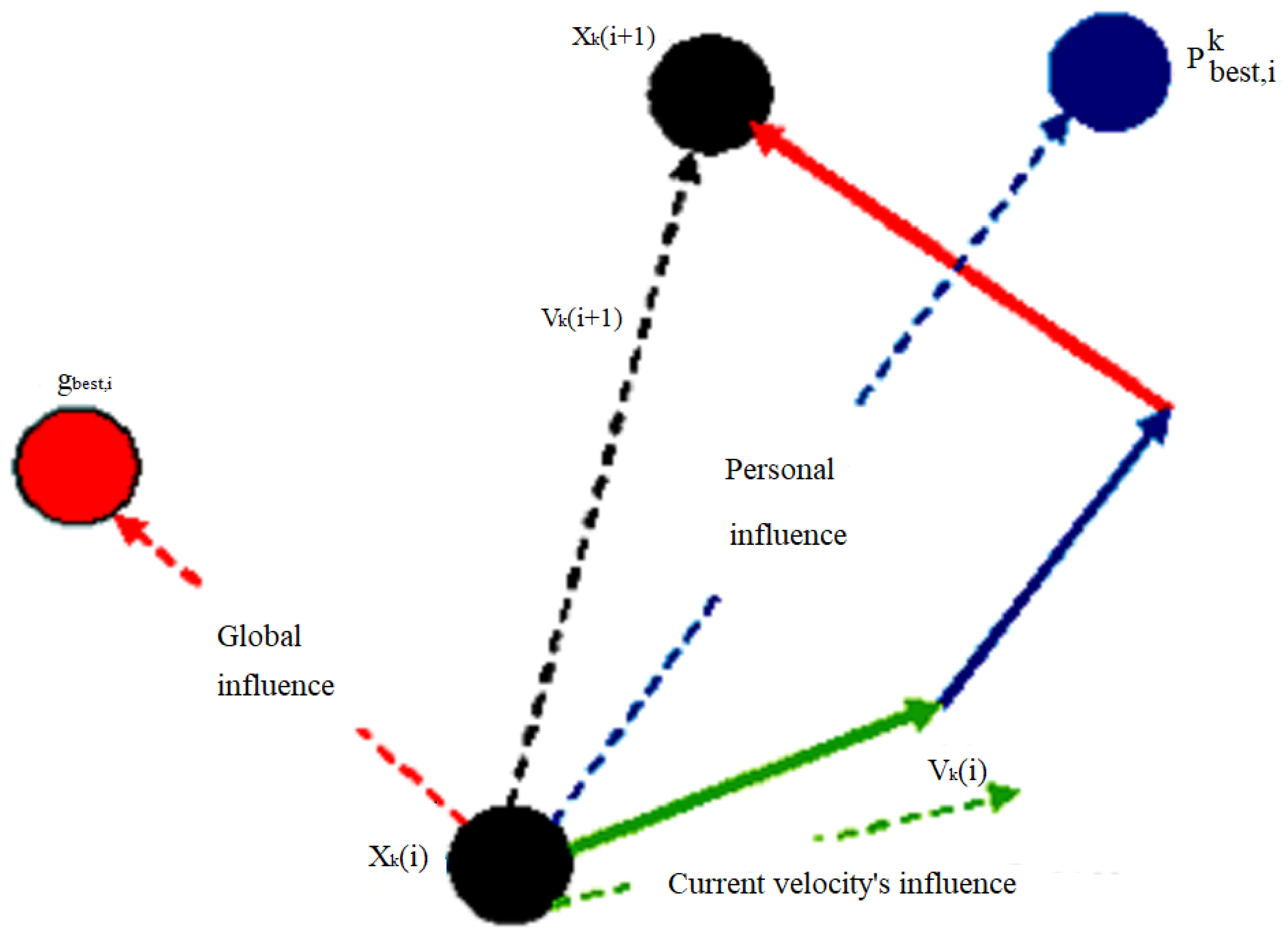
2.1. Updating of Velocity and Position of Particle in the Swarm

2.1.1. Updating of Velocity

In this algorithm, the regulation of velocity is considered as a major feature, as it is the main mechanism used to move the position of a particle to search for an optimal solution in the search space. Eberhart used the maximum values of velocity, and discussed results for different values of velocity. The velocity of particle k in the swarm in the (i + 1)th iteration, is updated, according to the following Equation (1):
V k ( i   +   1 )   = V k ( i   )     +   c 1   r 1 ( p b e s t , i k     X k ( i ) )   +   c 2   r 2 ( g b e s t , i     X k ( i ) )
where V k ( i   +   1 )   is the velocity of particle k at the (i + 1)th iteration; X k ( i ) is the position of particle k in the ith iteration; p b e s t , i k is individual best position of the particle k in the ith iteration; g b e s t , i is the global best position of the any particle in the ith iteration; c 1   a n d   c 2 are the real acceleration coefficients that control how much the global and individual best positions should influence the particle’s velocity; r 1   a n d   r 2 are uniformly distributed random numbers in the range 0 and 1, used to maintain an adequate level of diversity in the population. There are three components of the velocity update Equation (1) of kth particle in the (i + 1)th iteration, namely:
  • Momentum part;
  • Cognitive part;
  • Social part.
A brief description of the velocity equation has been illustrated in Table 2.

2.1.2. Updating the Position of Particle

The position of each particle k, at every iteration (i + 1)th, varies according to the following Equation (2):
X k ( i   +   1 )   =   X k ( i )   +   V k ( i   +   1 )  
where V k ( i   +   1 )   is the velocity of particle k at the (i + 1)th iteration; X k ( i + 1 ) is the position of particle k in the (i + 1)th iteration; X k ( i ) is the position of particle k in the ith iteration.
Figure 1 illustrates the state of swarm at the iteration (i + 1)th. It shows how the velocity of particle k is updated and that, in turn, updates the position of the kth particle in the iteration (i + 1)th.

2.2. Standard Particle Swarm Optimization (SPSO)

The authors Shi and Elberhart [14] introduced a new parameter ω , called the inertia weight of a particle. With this new parameter, the velocity update Equation (1) changed to Equation (3):
V k ( i   +   1 )   =   ω   V k ( i   )     +   c 1   r 1 ( p b e s t , i k     X k ( i ) )   +   c 2   r 2 ( g b e s t , i     X k ( i ) )  
The particle swarm optimization (PSO) algorithm with this improvement is commonly referred to as the standard PSO.

2.3. Pseudocode of PSO Algorithm

The Pseudocde of the particle swarm optimization algorithm is illustrated in the Algorithm 1 as follows:
Algorithm 1: The Pseudocde of the algorithm is as follows
INPUT: Fitness function, lower bound, upper bound is the part of problem i.e., it will be given in the problem. Np (Population Size), I (No. of iteration), ω, c 1   ,   c 2 are to be chosen by the user.
1.
Initialize a random population (P) and velocity (v) within the bounds;
2.
Evaluate the objective function value (f) of P;
3.
Assign p b e s t as P and f p b e s t as f;
4.
Identify the solution with best fitness and assign that solution as g b e s t and fitness as f g b e s t   .

For iteration:-
for i = 1 to I
         for k = 1 to Np
Determine the velocity ( v k ) of kth particle;
Determine the new position ( X k ) of kth particle;
Bound X k ;
Evaluate the objective function value f k of kth particle;
Update the population by including X k and f k ;
Update p b e s t k   and   f p b e s t     if   f k   <   f p b e s t k     then       { p b e s t k   =   X k f p b e s t     =   f k ;
Update g b e s t   and   f g b e s t     if   f p b e s t k     <   f g b e s t     then     { g b e s t   =   p b e s t k   f g b e s t     =   f p b e s t k   .
           end
end

2.4. Working Example of PSO

The PSO algorithm can be more understandable with a working example with some iterations. The example is illustrated as below:
Example: min f ( x )   =   x 1 2   +   x 2 2   + x 3 2   +   x 4 2                                 0 x i   10         i = 1 , 2 , 3 , 4
Solution: Parameter setting of PSO algorithm
Population Size ( N p ) = 5, Inertia Weight (w) = 0.7, Acceleration Coefficient = c 1   =   c 2 =   1.5 , Maximum iteration = 10
Iteration !: Generate random positions and velocities within domain 0 x i   10 and evaluate fitness of positions i.e.,
X ( position ) =   [ 4 0 0 8 3 1 9 7 0 3 1 5 2 1 4 9 6 2 8 3 ]   f ( X ) ( fitness function ) =   [ 80 140 35 102 113 ]   v ( velocity ) [ 9 6 1 8 5 1 3 0 7 4 1 4 3 0 2 1 1 6 8 7 ]  
Here fitness value of velocity is not required, fitness value of only positions is required
p b e s t ( 1 )   =   [ 4 0 0 8 3 1 9 7 0 3 1 5 2 1 4 9 6 2 8 3 ]                                                                     f p b e s t   =   [ 80 140 35 102 113 ]  
In the first iteration as we do not have any historical information, so current position is considered as best direction i.e., p b e s t   =   X .
Now, g b e s t   =   [ 0 3 1 5 ]                                                     f g b e s t   =   35
So, in iteration 1, we get:
V = [ 9 6 1 8 5 1 3 0 7 4 1 4 3 0 2 1 1 6 8 7 ] v 1 ( 1 ) v 2 ( 1 ) v 3 ( 1 ) v 4 ( 1 ) v 5 ( 1 )     X = [ 4 0 0 8 3 1 9 7 0 3 1 5 2 1 4 9 6 2 8 3 ]   X 1 ( 1 ) X 2 ( 1 ) X 3 ( 1 ) X 4 ( 1 ) X 5 ( 1 )   f ( X ) =   [ 80 140 35 102 113 ]  
p b e s t 1   =   [ 4 0 0 8 3 1 9 7 0 3 1 5 2 1 4 9 6 2 8 3 ] p b e s t ,   1 ( 1 ) p b e s t ,   2 ( 1 ) p b e s t ,   3 ( 1 ) p b e s t ,   4 ( 1 ) p b e s t ,   5 ( 1 )                                                                   f p b e s t   =   [ 80 140 35 102 113 ]
g b e s t   =   [ 0 3 1 5 ]                                                     f g b e s t   =   35
Iteration 2 (First solution):
To calculate v 1 ( 2 ) ,   X 1 ( 2 ) .
Let r 1   =     [ 0.4 0.3 0.9 0.5 ] and r 2   =     [ 0.8 0.2 0.7 0.4 ]
v 1 ( 2 ) =   w v 1 ( 1 )   +   c 1 r 1   ( p b e s t ,   1 ( 1 )     X 1 ( 1 ) )   +   c 2 r 2   ( g b e s t     X 1 ( 1 ) )   =   [ 1.5     5.1     1.75     3.8 ] X 1 ( 2 ) =   X 1 ( 1 )   +   v 1 ( 2 )     =   [ 4     0     0     8 ]   +     [ 1.5     5.1     1.75     3.8 ]   = [ 5.5     5.1     1.75     11.8 ] [ 0 , 10 ]
This is the new position of first particle in the second iteration but new position is not within the bounds.
So, by using corner bounding strategy
X 1 ( 2 )   =   [ 5.5 5.1 1.75 10 ] [ 0 , 10 ] f ( X 1 ( 2 ) )   =   159.32
No updation in p b e s t as f p b e s t ,   1 ( 2 )   =   159.32 >   f p b e s t ,   1 ( 1 )   =   80 and
No updation in g b e s t     g b e s t   = [ 0 3 1 5 ]   and f g b e s t   =   35
Iteration 2 (Second Solution):
To Calculate v 2 ( 2 ) ,   X 2 ( 2 )
v 2 ( 2 ) =   w v 2 ( 1 )   +   c 1 r 1   ( p b e s t ,   2 ( 1 )     X 2 ( 1 ) )   +   c 2 r 2   ( g b e s t     X 2 ( 1 ) )   =   [ 0.1 1.3 6.3 1.2 ] X 2 ( 2 ) =   X 2 ( 1 )   +   v 2 ( 2 )   = [ 3     1     9     7 ] +   [ 0.1     1.3     6.3     1.2 ]   = [ 2.9     2.3     2.7     5.8 ] [ 0 , 10 ] f ( X 2 ( 2 ) ) =   8.41 + 5.29 +   7.29 +   33.64 =   54.63
Update p b e s t as f p b e s t ,   2 ( 2 )   =   54.63 <   f p b e s t ,   2 ( 1 )   =   140
No updation in g b e s t   as f g b e s t   =   35   <   f p b e s t ,   2 ( 2 )   =   54.63
    g b e s t   = [ 0 3 1 5 ]   a n d   f g b e s t   =   35
Iteration 2 (Third Solution):
v 3 ( 2 )   =   w v 3 ( 1 )   +   c 1 r 1   ( p b e s t ,   3 ( 1 )     X 3 ( 1 ) )   +   c 2 r 2   ( g b e s t     X 3 ( 1 ) )         = [ 4.9     2.8     0.7     2.8 ]
X 3 ( 2 )   =   X 3 ( 1 )   +   v 3 ( 2 ) =   [ 0   3   1   5 ]   +     [ 4.9   2.8   0.7   2.8 ]     =   [ 4.9   5.8   1.7   7.8 ] [ 0 , 10 ] f ( X 3 ( 2 ) )   = 121.38
No updation in p b e s t as f p b e s t ,   3 ( 2 )   =   121.38 >   f p b e s t ,   3 ( 1 )   =   35
No updation in g b e s t ,     g b e s t   = [ 0 3 1 5 ]   a n d   f g b e s t   =   35
Iteration 2 (fourth Solution):
v 4 ( 2 ) =   w v 4 ( 1 )   +   c 1 r 1   ( p b e s t ,   4 ( 1 )     X 4 ( 1 ) )   +   c 2 r 2   ( g b e s t     X 4 ( 1 ) )   =   [ 0.3     0.6     1.75     1.7 ] X 4 ( 2 ) =   X 4 ( 1 )   +   v 4 ( 2 )   =   [ 2   1   4   9 ]   +     [ 0.3   0.6   1.75   1.7 ]   =   [ 1.7     1.6     2.25     7.3 ] [ 0 , 10 ] f ( X 4 ( 2 ) ) =   2.89 +   2.56 +   5.0625 +   53.29 =   63.8025
Update p b e s t as f p b e s t ,   4 ( 2 )   =   63.8025   <   f p b e s t ,   4 ( 1 )   =   102
No updation in g b e s t     g b e s t   = [ 0 3 1 5 ]   a n d   f g b e s t   =   35
Iteration 2 (Fifth Solution):
v 5 ( 2 )   =   w v 5 ( 1 )   +   c 1 r 1   ( p b e s t ,   5 ( 1 )     X 5 ( 1 ) )   +   c 2 r 2   ( g b e s t     X 5 ( 1 ) )   =   [ 6.5     4.5     1.75     6.1 ]
X 5 ( 2 )   =   X 5 ( 1 )   +   v 5 ( 2 )         =   [ 6     2     8     3 ]   +     [ 6.5     4.5     1.75     6.1 ] =   [ 0.5     6.5     6.25     9.1 ] [ 0 , 10 ]
  X 5 ( 2 )   =   [ 0 6.5 6.25 9.1 ] f ( X 5 ( 2 ) )   =   42.25 +   39.0625 +   82.81 =   164.1225
No updation in p b e s t as f p b e s t ,   5 ( 2 )   =   164.1225   >   f p b e s t ,   5 ( 1 )   =   113
No updation in g b e s t     g b e s t   = [ 0 3 1 5 ]   a n d   f g b e s t   =   35
So, in iteration 2, we get:
V = [ 1.5 5.1 1.75 3.8 0.5 1.3 6.3 1.2 4.9 2.8 0.7 2.8 0.3 0.6 1.75 1.7 6.5 4.5 1.75 6.1 ] v 1 ( 2 ) v 2 ( 2 ) v 3 ( 2 ) v 4 ( 2 ) v 5 ( 2 )   X   =     [ 5.5 5.1 1.75 10 2.9 2.3 2.7 5.8 4.9 5.8 1.7 7.8 1.7 1.6 2.25 7.3 0 6.5 6.25 9.1 ] X 1 ( 2 ) X 2 ( 2 ) X 3 ( 2 ) X 4 ( 2 ) X 5 ( 2 )   f ( X ) =   [ 159.32 54.63 121.38 63.8025 164.1225 ]
p b e s t ( 2 )   =   [ 4 0 0 8 2.9 2.3 2.7 5.8 0 3 1 5 1.7 1.6 2.25 7.3 6 2 8 3 ] p b e s t ,   1 ( 2 ) p b e s t ,   2 ( 2 ) p b e s t ,   3 ( 2 ) p b e s t ,   4 ( 2 ) p b e s t ,   5 ( 2 )                   f p b e s t   =   [ 80 54.63 35 63.8025 113 ]  
g b e s t   =   [ 0 3 1 5 ]                                                             f g b e s t   =   35
Iteration 3 (first Solution):
v 1 ( 3 )   =   w v 1 ( 2 )   +   c 1 r 1   ( p b e s t ,   1 ( 2 )     X 1 ( 2 ) )   +   c 2 r 2   ( g b e s t     X 1 ( 2 ) )         =   [ 6.45     0.645     1.925     1.16 ]  
X 1 ( 3 )   =   X 1 ( 2 )   +   v 1 ( 3 )   =   [ 5.5     5.1     1.75     10 ]   +     [ 6.45     0.645     1.925     1.16 ] =   [ 0.95     5.745     0.1725     11.16 ] [ 0 , 10 ]   =   [ 0     5.745     0     10 ] f ( X 1 ( 3 ) )   =   133.005025
No update in p b e s t   a s   f p b e s t ,   1 ( 3 )   =   133.005025   >   f p b e s t ,   1 ( 2 )   =   80
No update in g b e s t   a s   f g b e s t   =   35     g b e s t   = [ 0 3 1 5 ] and     f g b e s t   =   35
Iteration 3 (second Solution):
v 2 ( 3 )   =   w v 2 ( 2 )   +   c 1 r 1   ( p b e s t ,   2 ( 2 )     X 2 ( 2 ) )   +   c 2 r 2   ( g b e s t     X 2 ( 2 ) )         =     [ 3.55     1.12     6.195     1.32 ]   X 2 ( 3 )   =   X 2 ( 2 )   +   v 2 ( 3 )   =   [ 3.55     1.12     6.195     1.32 ]   +     [ 2.9     2.3     2.7     5.8 ]
=   [ 0.65     3.42     3.495     4.48 ] [ 0 , 10 ]   =   [ 0     3.42     0     4.48 ] f ( X 2 ( 3 ) )   =   11.6964 +   20.0704 =   31.7668
Update p b e s t as f p b e s t ,   2 ( 3 )   =   31.7668   <   f p b e s t ,   2 ( 2 )   =   54.63
Update g b e s t as f g b e s t   =   35   >     f p b e s t ,   2 ( 3 )   =   31.7668  
  g b e s t   =   [ 0 3.42 0 4.48 ]           f g b e s t   =   31.7668
Iteration 3 (third Solution):
v 3 ( 3 )   =   w v 3 ( 2 )   +   c 1 r 1   ( p b e s t ,   3 ( 2 )     X 3 ( 2 ) )   +   c 2 r 2   ( g b e s t     X 3 ( 2 ) )         =   [ 5.39     0.014     2.24     2.132 ]   X 3 ( 3 )   =   X 3 ( 2 )   +   v 3 ( 3 )   =   [ 4.9     5.8     1.7     7.8 ]   +   [ 5.39     0.014     2.24     2.132 ] = [ 0.49     5.786     0.54     5.668 ] [ 0 , 10 ]   = [ 0     5.786     0     5.668 ] f ( X 3 ( 3 ) )   =   33.4778 +   32.1262 = 65.604024
No updation in p b e s t as f p b e s t ,   3 ( 3 )   =   65.604024   >   f p b e s t ,   3 ( 2 )   =   35
No Updation in g b e s t       g b e s t   =   [ 0 3.42 0 4.48 ]   a n d   f g b e s t   =   31.7668
Iteration 3 (fourth Solution):
v 4 ( 3 )   =   w v 4 ( 2 )   +   c 1 r 1   ( p b e s t ,   4 ( 2 )   X 4 ( 2 ) )   +   c 2 r 2   ( g b e s t       X 4 ( 2 ) )         =   [ 2.25     0.966     3.5875     2.882 ]   X 4 ( 3 )   =   X 4 ( 2 )   +   v 4 ( 3 )   = [ 1.7     1.6     2.25     7.3 ]   +     [ 2.25     0.966     3.5875     2.882 ]   =   [ 0     2.566     0     4.418 ] f ( X 4 ( 3 ) )   =   26.10308
Update p b e s t as f p b e s t ,   4 ( 3 )   =   26.10308   <     f p b e s t ,   4 ( 2 )   =   63.8025
Update g b e s t as f g b e s t   =   35   > f p b e s t ,   4 ( 3 )   =   26.10308
  g b e s t   =   [ 0 2.566 0 4.418 ]   and     f g b e s t   =     26.10308
Iteration 3 (fifth Solution):
v 5 ( 3 )   =   w v 5 ( 2 )   +   c 1 r 1   ( p b e s t ,   5 ( 2 )     X 5 ( 2 ) )   +   c 2 r 2   ( g b e s t     X 5 ( 2 ) )         =   [ 0.95     0.0552     5.425     3.1142 ]   X 5 ( 3 )   =   X 5 ( 2 )   +   v 5 ( 3 )   =   [ 0     6.5     6.25     9.1 ]   +   [ 0.95     0.0552     5.425     3.1142 ] =   [ 0     6.4448     0.825     5.9858 ] f ( X 5 ( 3 ) )   =   78.045825
Update p b e s t as f p b e s t ,   5 ( 3 )   =   78.045825   <     f p b e s t ,   5 ( 2 )   =   113
No update in g b e s t
  g b e s t   =   [ 0 2.566 0 4.418 ] and f g b e s t   =     26.10308
So, in iteration 3:
V =   [ 6.45 0.645 1.925 1.16 3.55 1.12 6.195 1.32 5.39 0.014 2.24 2.132 2.25 0.966 3.5875 2.882 0.95 0.0552 5.425 3.1142 ] v 1 ( 3 ) v 2 ( 3 ) v 3 ( 3 ) v 4 ( 3 ) v 5 ( 3 ) ,
X = [ 0 5.745 0 10 0 3.42 0 4.48 0 5.786 0 5.668 0 2.566 0 4.418 0 6.4448 0.825 5.9858 ] X 1 ( 3 ) X 2 ( 3 ) X 3 ( 3 ) X 4 ( 3 ) X 5 ( 3 )       f ( X ) =   [ 133.005 31.7668 65.604024 26.10308 78.046 ]
p b e s t ( 2 )   =   [ 4 0 0 8 0 3.42 0 4.48 0 3 1 5 0 2.566 0 4.418 0 6.4448 0.825 5.9858 ] p b e s t ,   1 ( 3 ) p b e s t ,   2 ( 3 ) p b e s t ,   3 ( 3 ) p b e s t ,   4 ( 3 ) p b e s t ,   5 ( 3 )           f p b e s t   =   [ 80 31.7668 35 26.103088 78.046 ]
Similarly, other iterations can be performed. This example is solved completely up to the third iteration only. This is the just the explanation of the working of particle swarm optimization (PSO) algorithm through an example. It is not possible to obtain an optimal solution by manual calculations. Further iterations can be performed through proper software for the PSO algorithm.

3. Parameters of PSO

There are a number of control parameters in the particle swarm optimization (PSO) algorithm, namely the number of particles, size of neighborhood, number of iterations, acceleration coefficients, inertia weight, dimension of the problem and random values associated with the cognitive and social component of the velocity update equation. In addition, if velocity clamping and constriction are used, then maximum velocity and coefficient of constriction are also considered to be very effective control parameters (Engelbrecht, A.P.) [15]. These parameters have a great impact on the convergence speed, performance and quality of the solution obtained. The fine tuning of the parameters is required, to avoid premature convergence. Discussions of these parameters are as below:

3.1. Population Size

Swarm size (ns) is the number of particles in the whole swarm. A large number of the particles cover a larger part of the search space per iteration, but it also increases the computational complexity per iteration. It can also be possible that a larger number of particles may lead to a lesser number of iterations to obtain an optimal solution. From the heuristics found in the publications, the success rate of getting a good solution in the PSO algorithm is greater with a swarm size of 20 to 50 particles (Eberhart and Shi) [16]. However, it is also found that the optimal population size is usually problem dependent.

3.2. Number of Iterations

In the same way as the swarm size, the number of iterations is also problem dependent, to obtain a good solution in the particle swarm optimization (PSO) algorithm. On the one hand, a lesser number of iterations may prematurely stop the search process, and on the other hand, a larger number of iterations only adds to the computational complexity in obtaining a quality solution, if the termination criterion depends on a number of iterations.

3.3. Neighborhood Size

The size of the neighborhood is related to the degree of social interaction among the swarm members. The less interaction that there is in a neighborhood of a smaller size leads to a slow but reliable convergence. The more interaction that there is in a neighborhood of a larger size leads to a fast convergence. For instance, if the size of a neighborhood is defined as two, then particle (k) compares its fitness value with particle (k − 1) and particle (k + 1) (Eberhart and Shi) [16]. From the heuristics found in the publications, the size of a neighborhood is usually taken to be 15% of the population size in most of the applications.

3.4. Acceleration Coefficients

The impact of the cognitive and social component on the particle’s velocity is managed by the acceleration coefficients c 1   a n d   c 2 , along with the random numbers, r 1   a n d   r 2 . A proper balance between the values of c 1   a n d   c 2 is required, as inappropriate values of c 1   a n d   c 2 may result in divergent and cyclic behavior of the whole swarm. Impact of different values of c 1   a n d   c 2 is explained in Table 3.

3.5. Velocity Clamping

It is the property of a good optimization algorithm to create an optimal balance between the exploration and exploitation objectives. It was found in the basic PSO algorithm that the velocity quickly explodes to larger values and, as a result of it, the position of the particle changes rapidly, that leads to the divergence of the whole swarm. To overcome this problem, Eberhart and Kennedy [16] introduced the concept of velocity clamping i.e., the velocities are clamped to stay within the boundary constraints. Vmax denotes the maximum allowed velocity that creates a better equilibrium between the global exploration and local exploitation. If the velocity of the particle reaches beyond this specified limit Vmax, then that velocity of the particle is set to the maximum velocity value (Vmax). Vmax is an important parameter as it controls the explosion of velocity. Higher values of Vmax encourage global exploration, but it may risk the possibility that the particles may miss a better search area. Since the particles are moving faster, they may jump over the optimal solution and continue to roam in a useless region in the global search area, and on the other hand, the smaller values of Vmax encourage local exploitation but may risk the possibility that the particles become trapped in the local optima, resulting in the particles not exploring a better search space. So, to create a balance between exploration and exploitation, an appropriate value of Vmax is required.
We can write Vmax as written in Equation (4):
Vmax = δ (Xmax − Xmin)
where Xmax and Xmin are, respectively, the maximum and minimum values of X and δ ε (0, 1].

3.6. Constriction Coefficient

To ensure and enhance the convergence speed of the PSO algorithm and to ensure a balance between exploration and exploitation, Maurice Clerc [17] suggested the parameter constriction coefficient χ (Clerc and Kennedy) [18]. He implemented it on the basic velocity update Equation (1) of the original PSO algorithm.
The velocity update Equation (1) changes to Equation (5):
V k ( i   +   1 )   =   χ   [ V k ( i   )     +   c 1   r 1 ( p b e s t , i k     X k ( i ) )   +   c 2   r 2 ( g b e s t , i     X k ( i ) ) ]  
where the constriction coefficient χ is given by
χ   =   2 κ | 2     φ     φ   ( φ     4 ) |
where φ =   φ 1   +   φ 2 and φ 1     =   c 1   r 1 , φ 2     =   c 2   r 2 , κ is a function of c 1   and   c 2 .
Equation (6) is used under the condition that φ 4 and κ     [ 0 , 1 ] .
Parameter κ controls the exploitation and exploration abilities of the swarm. If κ ≈ 0 then the convergence is faster with local exploitation, and if κ ≈ 1 then the convergence is slow with a higher degree of exploration. Usually κ is set to a constant value. However, a higher degree of exploration with local exploitation can be achieved by taking the initial value of κ near to 1, then decreasing it to 0. When Clerc’s constriction factor is used with the PSO algorithm, then φ   =   4.1 a n d   t h u s   c o n s t a n t     m u l t i p l i e r     κ   0.729 .

3.7. Inertia Weight

The notion of inertia weight ‘ω’ of a particle in the basic PSO algorithm was first introduced into the literature by Shi and Eberhart [14], to improve its convergence performance. This coefficient controls the global and local exploration and the exploitation capacity of the swarm, by determining the influence of the previous velocity on the particle’s current movement. With the introduction of this new parameter ω, the velocity update Equation (1) is changed to velocity update Equation (3). The suitable value of ω results in fewer iterations on average to find a sufficiently optimal solution. To balance the global and local search and to ensure the convergence to a sufficiently optimal solution in a lesser number of iterations, an adjustment in the value of the inertia weight ω, is extremely important. Larger values of ω facilitate the global exploration and smaller values promote the local exploitation. As originally proposed, the value of the inertia weight ω is often decreased linearly from about 0.9 (ωmax) to 0.4 (ωmin) during a run.
It is described as follows Equation (7) (Eberhart and Shi [19]):
ω   =   ω m a x     ω m a x   ω m i n i t e r m a x ×   i t e r
where i t e r m a x is the maximum number of iterations, iter is the current iteration, ω m a x and ω m i n are initial and final values of the inertia weight respectively.
Van den Bergh and Engelbrecht [20] stated a strong relationship ( see Equation (8)) between acceleration coefficients c1, c2 and inertia weight ω as:
ω   >   1 2   (   c 1   +   c 2 )     1  
Eberhart and Shi [19] made a comparison between the constriction coefficient ( χ ) and inertia weight ( ω ). The authors considered that both of the approaches are equally effective. As both the constriction coefficient and inertia weight aim to create a balance between the exploration and exploitation capabilities, this results in an improvement in the convergence time and quality of solution obtained. Low values of the constriction coefficient and inertia weight result in exploitation, whereas higher values result in exploration. Eberhart and Shi [19] also proved that if velocity clamping and constriction coefficient are used together, even then convergence can be faster.

4. Advances on Particle Swarm Optimization (PSO) Algorithm

Due to the simplicity and wide range of applications of the particle swarm optimization (PSO) algorithm, it has gained more attention from a variety of researchers belonging to different fields. Houssein et al. [21] presented a rigorous and systematic review on the developments, recent trends, hybridization, parallelization and diverse applications of the particle swarm optimization (PSO) algorithm. Many researchers are working on the advancement of the PSO algorithm. As a result, more research is being completed in this area, that has led several researchers to report problems with the original PSO algorithm, such as premature convergence, performance issues, etc. In order to lessen these types of problems and improve its effectiveness and efficiency, researchers have made many advances on the original PSO algorithm. The advances on PSO algorithm have been sectioned into four categories:
  • Modifications of original PSO;
  • Extensions of applications of PSO;
  • Theoretical analysis on PSO;
  • Hybridization of PSO.

4.1. Modifications of Original PSO

There are modifications of the PSO algorithm, including fuzzy PSO, bare-bones PSO, etc. Krohling and Renato [22] made a modification in the original particle swarm algorithm by introducing the concept of Gaussian probability distribution. In their proposed algorithm, they only needed the parameter ‘the number of particles’ to be specified before actually using the algorithm. The experimental results of the Gaussian particle swarm algorithm showed that the Gaussian swarm outperformed the standard PSO. Baskar and Suganthan [23] introduced a new version of the PSO, called concurrent PSO (CONPSO), to improve the convergence performance of the original PSO. By testing this new version of the PSO on six classical functions, the authors proved that this new version of the PSO, i.e., the CONPSO, outperformed many other approaches of PSO. Kennedy and Eberhart [24] reworked the original particle warm optimization (PSO) technique and introduced a binary particle swarm. According to the authors, this new version of the PSO algorithm could optimize any function, continuous or discrete. They discussed this algorithm with various examples and applications. To make the basic particle swarm algorithm more understandable, Kennedy [25] eliminated the velocity formula. The author compared several variations and discovered its similarity with other stochastic population-based problem-solving methods, and suggested new avenues of investigation.
Mendes et al. [26] modified the original PSO algorithm by the concept of fully informed particles in the original PSO, as they felt that each of the particles in the swarm need not be affected only by the best performer among his neighbors. With the help of numerical experiments, the authors revealed that this new modified version of PSO outperformed the original PSO. Cervantes et al. [27] proposed to resolve the classification problems by making some modifications in the original PSO. So, a binary version of the PSO algorithm was compared with some machine-learning techniques, and the authors showed the promising results. Shi and Eberhart [28] made use of a fuzzy system to adopt the inertia weight of the particle swarm optimization (PSO) algorithm and introduced a new variant of PSO, called fuzzy adaptive PSO. Experiments on three test functions concluded that this fuzzy adaptive PSO was a promising optimization technique.
To detect facial emotion, Ghandi et al. [29] presented a novel approach called guided particle s optimization (GPSO) by modifying the original particle swarm optimization (PSO) algorithm. The authors proved that their emotion detection algorithm gave promising results in terms of accuracy in the detection of emotions. In order to obtain an optimum solution, Tanweer et al. [30] derived a new PSO algorithm, namely the self-regulating PSO (SRPSO) algorithm, by incorporating the best of the human-learning strategies. The authors proposed the learning strategies, on the one hand using a self-regulatory inertia weight for better exploration, and on the other hand using self-perception of the global search space for better exploitation. The statistical analyses indicated the superiority of the SRPSO over other metaheuristics. Presently, many researchers are also working on the further modification of the original PSO algorithm.

4.2. Extensions of Applications of PSO

Since its origin in 1995, researchers have also widened/extended the range of application of the original PSO algorithm to a variety of optimization problems, such as constrained, multi objective, multi modal, discrete and binary optimization. To solve the multi-objective optimization problems, Seok et al. [31] introduced a modified variant of the PSO algorithm, namely the homogeneous particle swarm optimizer (HPSO). The authors proved the excellent exploration ability of the proposed algorithm with other multi-objective PSO algorithms by making a comparison study. The authors, Coello and Lechuga [32], extended the application of the original particle swarm optimization (PSO) to solve the multi-objective optimization problems by using a Pareto dominance approach to determine the flight direction of the particle. By testing it with some standard test functions, the authors concluded that their approach was highly competitive in comparison to the other multi-objective optimization techniques. Mohamed et al. [33] proposed a new algorithm by hybridizing particle swarm optimization (PSO) with two other statistical techniques—Ranking and Selection (R&S), and Mean Square Error Criterion (MSE), in order to solve the stochastic optimization problems, called (STPSO). The authors proved the robustness of their proposed algorithm with experimental results. In order to solve the NP hard knapsack problems (KPs), Bansal and Deep [34] designed a modified binary particle swarm optimization (MBPSO) algorithm. The authors tested this new modified binary PSO version on 10 benchmark problems, and by comparing the results with both the binary particle swarm optimization (BPSO) and the genotype phenotype-modified binary particle swarm optimization (GPMBPSO), showed its effectiveness in terms of reliability, cost and the quality of the solution obtained over the other algorithms.
To efficiently solve the different problems on power systems, Rahmani et al. [35] proposed an evolutionary modified particle swarm optimization. On the basis of numerical experiments, the authors proved that their proposed algorithm was efficiently able to solve the constrained economic dispatch (ED) problem with a comparatively higher rate of convergence than the basic PSO. To efficiently solve the clustering problem, Neshat and Yazdi [36] proposed a new cooperative algorithm that utilized the global search ability of the PSO algorithm and the local search ability of k-means. The authors made a comparison of their proposed algorithm with other algorithms, such as PSO with constriction factor (CF-PSO) and k-means algorithms and revealed the convergence efficiency of their proposed algorithm. In order to solve the university course timetabling problems using PSO, the authors, Kanoh and Chen [37], introduced a new algorithm, using transition probability into the basic PSO algorithm. With the help of the experimental results, the authors demonstrated the effectiveness of their proposed algorithm over evolutionary strategy to solve the time-table problems. Garsva and Danenas [38] presented a new PSO algorithm by using a linear SVM (support vector machine) approach to solve both small and large scale classification problems. On the basis of the experiments, the authors concluded that their proposed PSO-LinSVM approach gave comparatively better results than other similar approaches.
The basic PSO algorithm does not work well for solving problems of mobile robot path planning, due to its slow convergence and limitations on application. To overcome this, the authors, Li et al. [39], derived the improved particle swarm optimization (IPSO) algorithm. By making a comparative study with other approaches on the standard benchmark functions, the authors proved that their derived algorithm gave a better solution with a lower number of iterations. In order to monitor the conditions of the surge arrester, Hoang et al. [40] proposed a novel differential particle swarm optimization(PSO)-based support vector machine (SVM) classifier, namely (DPSO-SVM). The authors, through experiments on several benchmark functions, showed the superiority of the proposed algorithm (DPSO-SVM) in order to improvise the classifier’s performance. In neuro fuzzy system (NFS), usually a gradient-based algorithm was used by the researchers, but Karakuzu et al. [41] used an improved PSO (iPSO) to introduce the first embedded high-speed, low-cost implementation of the neuro fuzzy network (NFN) hardware through online training on a field programmable gate array (FPGA). The authors tested its proposed implementation method on practical problems. The results showed the efficiency of the proposed implementation over other approaches available in the literature. In order to solve a power consumption minimization problem, Liao et al. [42] suggested a PSO-based algorithm, namely distribution PSO (DPSO). The improved algorithm of PSO was checked on a luminous control problem and the results showed the effectiveness of the modified algorithm, along with its suitability to be parallelized. The same optimization problem performed differently with different settings of the parameters. Based on the concept of the building block thesis, Li et al. [43] proposed two variants to the PSO algorithm, namely the PSO with a fixed phase (PSOFP) algorithm, and the PSO with a dynamic phase (PSODP) algorithm. These new variants were tested on benchmark functions to solve the single objective numerical optimization, and revealed the robustness of the proposed variant of the PSO algorithm.
The areas of application for the PSO algorithm has been extended by many researchers, but there is still a need to explore more areas of application of the PSO algorithm.

4.3. Theoretical Analysis on PSO

By realizing the importance of the appropriate values of the control parameters in the PSO algorithm, such as the inertia weight, acceleration coefficients, number of particles, etc., the researchers diverted their attention towards the theoretical aspects of the PSO algorithm and derived many theories related to parametric selection to obtain an optimal solution in a lower number of iterations and with a higher rate of convergence. Their theoretical analysis includes parametric setting, convergence analysis, etc. Shi and Eberhart [14] had proposed a new PSO parameter, called inertia weight ‘ ω ’ into the original particle swarm optimizer to improve its convergence performance. The authors explained the impact of this new parameter through examples. Shi and Eberhart [44] investigated the convergence performance of the particle swarm optimization (PSO) algorithm with a linearly decreasing inertia weight, and tested it on four non-linear functions. On the basis of the results, the authors concluded that some of the disadvantages of PSO could be overcome by adjusting the inertia weight. By obtaining motivation from the Gaussian and Cauchy probability distribution in the PSO algorithm, the authors Krohling and Coelho [45] proposed a modified variant of the PSO, namely PSO-E, that made use of the exponential probability distribution to upgrade the convergence performance. The numerical results on well-known classical functions indicated the competence of PSO-E in finding the solution in a lower number of iterations. Feng et al. [46] proposed a new adaptive inertia weight approach in the particle swarm optimization (PSP) algorithm. The performance of this newly proposed variant of PSO was checked on three classical benchmark functions and the results were also analyzed to prove its higher speed of convergence and more capability in locating the optimal solution in comparison to other optimization techniques. In order to balance between the local exploitation and the global exploration abilities for the PSO variant, Qin et al. [47] introduced a modified variant of PSO, called the adaptive inertia weight PSO algorithm (AIW-PSO). The authors proved the efficiency of the proposed algorithm (AIW-PSO) by comparing its results with other modified variants of the PSO, namely fuzzy adaptive inertia weight PSO, random number inertia weight PSO and linearly decreasing inertia weight PSO. The results showed that this new algorithm, AIW-PSO, outperformed the other algorithms.
Keeping in mind the importance of the parameter inertia weight in the PSO, Jiao et al. [48] proposed a dynamic inertia weight particle swarm optimization algorithm. The authors tested their improved PSO on six classical problems and concluded that the proposed variant improved the search performance of the standard particle swarm optimization (SPSO) algorithm.
Inertia weight is considered to be the most important parameter in the PSO algorithm. Usually, ω is chosen to be of small value in the range [0, 1] but Deep et al. [49] considered varying the values of ω, and proposed two variants of PSO, namely the globally adaptive inertia weight (GAIW) PSO and the locally adaptive inertia weight (LAIW) PSO. By testing these variants on various benchmark problems, the authors concluded that the proposed variant outperformed the basic PSO in terms of accuracy, efficiency and convergence speed. To improvise the convergence speed and to overcome the stagnation behavior of the basic PSO algorithm, Deep et al. [50] proposed a new variant of the basic PSO called fine grained inertia weight PSO (FGIWPSO). By testing their proposed variant of PSO on ten benchmark functions, the authors showed its effectiveness over the basic PSO, in terms of the quality of the solution obtained and the rate of convergence. To overcome the disadvantages of premature convergence of the PSO, Isiet and Gadala [51] conducted an extensive sensitivity analysis on the impact of the control parameters of the PSO algorithm. For parametric analysis, the authors considered a constraint optimization problem, and discovered that the PSO is most sensitive to inertia weight (ω) and acceleration coefficients (c1 and c2), and therefore suggested some optimal parametric combinations, and on the basis of a verification study of the suggested parameters showed that the proposed PSO could outperform some other metaheuristics.

4.4. Hybridization of PSO Algorithm

When the PSO algorithm is combined with some traditional and evolutionary optimization algorithms, in order to improve the effectiveness and efficiency of the algorithm and to compensate for the weakness of each other, then that is termed as the hybridization of the PSO. One can also say that combining the advantages of the PSO with the advantages of another optimization algorithm is called the hybridization of PSO algorithm, or the blending of the PSO with another optimization algorithm. The researchers hybridized PSO with many other algorithms, including the genetic algorithm (GA), the differential evolution (DE), the Ant Colony optimization (ACO), the simulated annealing (SA), the artificial Bee colony (ABC), etc. and found very promising results.
Nowadays, the PSO has become one of the researchers’ choices for the purposes of hybridization. Deep and Bansal [52] introduced the qPSO algorithm by hybridizing the PSO with a quadratic approximation operator. The authors considered the two variants of the PSO algorithm, namely the PSO with linearly decreasing inertia (PSO-W) and the PSO with constriction factor (PSO-C) for the purpose of hybridization, and proposed two new variant of PSO, namely qPSO-W and qPSO-C. The performance of the proposed variant was tested on 15 benchmark problems. The numerical results showed that the new hybrid PSO variants outperformed the basic PSO variants. For the purpose of microgrid optimization, Bao et al. [53] compared their proposed Multi-PSO-SVM prediction model with the other three algorithms and proved its superiority over them. To force the PSO algorithm to jump out of the stagnation situation, Liua et al. [54] hybridized particle swarm optimization (PSO) with differential evolution (DE) and proposed a novel hybrid algorithm, namely PSO-DE. On the basis of numerical experiments on constrained numerical and engineering optimization functions, the authors showed that their proposed novel approach resolved the convergence issues of basic PSO and also improved the quality of the solution obtained.
To overcome the various problems related to the PSO algorithm, Pu et al. [55] proposed an HPSO algorithm, and with experimental results proved the higher rate of stability, clustering efficiency and the global search ability of their algorithm over others. By using python tools, Mao et al. [56] developed a PSO-LSTM-based model to investigate the speed of road traffic in Kunming City, China. Singh et al. [57] introduced a new hybrid version of the particle swarm optimization (PSO) algorithm, namely the hybrid particle swarm optimization (HPSO) by combining two different approaches of PSO i.e., standard particle swarm optimization (SPSO) and mean particle swarm optimization (MPSO). By conducting numerical experiments on several benchmark problems, the authors concluded that that their proposed algorithm worked efficiently in comparison to SPSO and MPSO, in terms of speed and quality of solution. For the purpose of grid scheduling and resource management, Ankita and Sahana [58] proposed a PSO-based Ba-PSO scheduling algorithm. Song et al. [59] introduced a PSO-SVM regression model and proved its higher accuracy by proving that the average relative errors of the regression results of the specific supported roadway i.e., the wood-supported roadway, the I-steel-supported roadway and the bolt-net-supported roadway were all <5%.
Yang [60] proposed an improved PSO-BP combined forecasting model. This newly combined forecasting model is used in the college student entrepreneurship prediction experiment. Pozna et al. [61] presented a hybrid version of PSO, namely Particle Filter-Particle Swarm Optimization (PF-PSO) algorithm and proved its application to the fuzzy-controlled servo system. To obtain an optimal solution for the dynamic facility layout problem (DFLP), Nasab and Emami [62] proposed a hybrid PSO (HPSO) that mapped the discrete feasible space of the DFL problem into a continuous space with the help of coding procedure, and after that, the search for good quality solutions of the problem. For further improvements in their proposed algorithm, the authors combined it with simulated annealing. With the help of different experiments using their proposed algorithm, they proved that it was comparatively efficient compared to other variants. To create a balance between the global and local search abilities, Esmin and Matwin [63] proposed a hybrid PSO algorithm (HPSOM) by integrating PSO with a genetic algorithm, using the mutation process. On the basis of the numerical experiment, the authors showed that their proposed method significantly outperformed SPSO in terms of factors such as convergence speed, stability and the quality of the solution obtained.
In order to stabilize the stability of the power system, Elazim and Ali [64] hybridized the particle swarm optimization (PSO) and the bacterial foraging optimization algorithm (BFOA), and proposed a new version, namely the bacterial swarm optimization (BSO). To check the validity of the proposed version BSO, numerical experiments were conducted by the authors and the results presented the effectiveness of the proposed controller over the original PSO and BFOA algorithm. In order to optimize the learning rate of the neural network, Enireddy and Kumar [65] combined the cuckoo search algorithm with the particle swarm optimization (PSO) algorithm and proposed an improved image classification algorithm for content-based image retrieval (CBIR). On the basis of the experimental results, the authors showed the classification accuracy and faster learning with this proposed neural network algorithm.
Garg [66] proposed a guided hybrid approach, namely a PSO-GA algorithm, in order to solve the constrained optimization problems. On the basis of a comparative study conducted on various engineering design optimization problems, the author proved the effectiveness of the proposed algorithm over other evolutionary algorithms in searching for the near optimal global solution. Singh and Singh [67] proposed a new hybrid variant of particle swarm optimization (PSO) and the Grey Wolf optimizer (GWO), namely the HPSOGWO, by using exploitation capabilities from PSO and exploration capabilities from GWO. The authors tested their newly derived hybrid variant on 23 classical problems and by their experimental results showed that the newly developed variant outperformed other algorithms in respect of convergence and the accuracy of the solution obtained. Al-Thanoon et al. [68] presented a new hybrid algorithm by combining the advantages and strengths of both the particle swarm optimization (PSO) algorithm and the firefly algorithm (FFA), to provide a balance between the exploration and exploitation capabilities. The authors compared the performance of the newly proposed algorithm with the standard particle swarm optimization (PSO) algorithm and firefly algorithm (FFA) and yielded better results by proving its efficiency in obtaining a high classification performance.
To solve different nonlinear and convex optimal power flow (OPF) problems, Khan et al. [69] introduced an effective and novel hybrid firefly particle swarm optimization (HFPSO) algorithm. They coded their technique, using MATLAB software, and checked its effectiveness on several test functions, and showed that the proposed algorithm had a faster rate of convergence and had more capability to handle several complex OPF problems. Qinghai [70] explained the basic principles of the PSO algorithm, and discussed its advantages and disadvantages. He discussed some of the improved and hybrid versions of the standard particle swarm optimization (SPSO) algorithm and suggested its future research scope. Nowadays, researchers are working more in the area of hybridization, because hybridization makes it possible to combine the advantages of the hybridized algorithms by setting aside their weaknesses, leading to the development of a highly efficient hybridized algorithm.

5. Conclusions

On the one hand particle swarm optimization (PSO) algorithm is popular among the scientific community, due to its simplicity, easy implementation and competence to be applied to a wide range of problems. On the other hand, the modifications, extensions and hybridization of the PSO algorithm during the last few decades indicates that there are a lot more opportunities to make improvements to the algorithm, to increase the effectiveness of the results. The researchers have worked on the limitations of the PSO algorithm, such as obtaining trapped in the local optima, premature convergence, impropriate accuracy, etc. The researchers have tried to make it more applicable to more classes of optimization problems. In the present paper, by presenting an overview of the PSO algorithm, we have explained the basic concepts and parameters of PSO, along with a variety of the advancements of the PSO algorithm. From the current literature survey on the PSO algorithm, we have also found that a large amount of research has been carried out on the PSO algorithm, but more areas of the applications of PSO can be enhanced in the future research. Research both on the applications aspect and the hybridization of the algorithm can also be conducted. The theoretical aspect can also be further explored in future research, in order to lessen the number of known parameters and criteria of their selection for the easy implementation of the particle swarm optimization (PSO) algorithm to its wide range of applications.

Author Contributions

S.B.S. conceived the idea to write the review on achievement of Particle Swarm Optimization Algorithm. M.J. prepared the draft version of this article. All the authors revised and finalized the final draft of the manuscript. All authors have read and agreed to the published version of the manuscript.

Funding

For this research work, there is no external funding agency.

Institutional Review Board Statement

Not applicable.

Informed Consent Statement

Informed consent was obtained from all individual participants involved in this study.

Data Availability Statement

Not applicable.

Conflicts of Interest

The authors declare no conflict of interest.

References

  1. Zhao, W.; Wang, L.; Mirjalili, S. Artificial hummingbird algorithm: A new bio-inspired optimizer with its engineering applications. Comput. Methods Appl. Mech. Eng. 2022, 388, 114194. [Google Scholar] [CrossRef]
  2. Jia, H.; Sun, K.; Zhang, W.; Leng, X. An enhanced chimp optimization algorithm for continuous optimization domains. Complex Intell. Syst. 2022, 8, 65–82. [Google Scholar] [CrossRef]
  3. Dhiman, G.; Garg, M.; Nagar, A.; Kumar, V.; Dehghani, M. A novel algorithm for global optimization: Rat Swarm Optimizer. J. Ambient. Intell. Humaniz. Comput. 2020, 12, 8457–8482. [Google Scholar] [CrossRef]
  4. Abdollahzadeh, B.; Gharehchopogh, F.S.; Mirjalili, S. African vultures optimization algorithm: A new nature-inspired metaheuristic algorithm for global optimization problems. Comput. Ind. Eng. 2021, 158, 107408. [Google Scholar] [CrossRef]
  5. Bhardwaj, S.; Kim, D.-S. Dragonfly-based swarm system model for node identification in ultra-reliable low-latency communication. Neural Comput. Appl. 2021, 33, 1837–1880. [Google Scholar] [CrossRef]
  6. MiarNaeimi, F.; Azizyan, G.; Rashki, M. Horse herd optimization algorithm: A nature-inspired algorithm for high-dimensional optimization problems. Knowl. Based Syst. 2021, 213, 106711. [Google Scholar] [CrossRef]
  7. Mohamed, A.W.; Hadi, A.A.; Mohamed, A.K. Gaining-sharing knowledge based algorithm for solving optimization problems: A novel nature-inspired algorithm. Int. J. Mach. Learn. Cybern. 2020, 11, 1501–1529. [Google Scholar] [CrossRef]
  8. Martínez-Álvarez, F.; Asencio-Cortés, G.; Torres, J.F.; Gutiérrez-Avilés, D.; Melgar-García, L.; Pérez-Chacón, R.; Rubio-Escudero, C.; Riquelme, J.C.; Troncoso, A. Coronavirus optimization algorithm: A bioinspired metaheuristic based on the COVID-19 propagation model. Big Data 2020, 8, 308–322. [Google Scholar] [CrossRef]
  9. Heidari, A.A.; Mirjalili, S.; Faris, H.; Aljarah, I.; Mafarja, M.; Chen, H. Harris hawks optimization: Algorithm and applications. Future Gener. Comput. Syst. 2019, 97, 849–872. [Google Scholar] [CrossRef]
  10. Odili, J.B.; Kahar, M.N.M.; Anwar, S. African Buffalo Optimization: A Swarm-Intelligence Technique. Procedia Comput. Sci. 2015, 76, 443–448. [Google Scholar] [CrossRef] [Green Version]
  11. Eiben, A.E.; Schippers, C.A. On evolutionary exploration and exploitation. Fundam. Inform. 1998, 35, 35–50. [Google Scholar] [CrossRef]
  12. Wolpert, D.H.; Macready, W.G. No free lunch theorems for optimization. IEEE Trans. Evol. Comput. 1997, 1, 67–82. [Google Scholar] [CrossRef] [Green Version]
  13. Kennedy, J.; Eberhart, R. Particle Swarm Optimization. In Proceedings of the IEEE International Conference on Neural Networks, Perth, WA, Australia, 27 November–1 December 1995; IEEE Press: Piscataway, NJ, USA, 1995; pp. 1942–1947. [Google Scholar]
  14. Shi, Y.; Eberhart, R.C. A Modified Particle Swarm Optimizer. In Proceedings of the IEEE International Conference on Evolutionary Computation, Anchorage, AK, USA, 4–9 May 1998; IEEE Press: Piscataway, NJ, USA, 1998; pp. 69–73. [Google Scholar]
  15. Engelbrecht, A.P. Computational Intelligence: An Introduction; John Wiley and Sons: Hoboken, NJ, USA, 2007; Chapter 16; pp. 289–357. [Google Scholar]
  16. Eberhart, R.C.; Shi, Y. Particle Swarm Optimization: Developments, Applications and Resources. In Proceedings of the IEEE Congress on Evolutionary Computation, Seoul, Korea, 27–30 May 2001; Volume 1, pp. 27–30. [Google Scholar]
  17. Clerc, M. The Swarm and the Queen: Towards a Deterministic and Adaptive Particle Swarm Optimization. In Proceedings of the IEEE Congress on Evolutionary Computation, Washington, DC, USA, 6–9 July 1999; Volume 3, pp. 1951–1957. [Google Scholar]
  18. Clerc, M.; Kennedy, J. The Particle Swarm-Explosion, Stability, and Convergence in a Multidimensional Complex Space. IEEE Trans. Evol. Comput. 2002, 6, 58–73. [Google Scholar] [CrossRef] [Green Version]
  19. Eberhart, R.C.; Shi, Y. Comparing Inertia Weights and Constriction Factors in Particle Swarm Optimization. In Proceedings of the IEEE Congress on Evolutionary Computation, La Jolla, CA, USA, 16–19 July 2000; Volume 1, pp. 84–88. [Google Scholar]
  20. Van den Bergh, F.; Engelbrecht, A.P. A Study of Particle Swarm Optimization Particle Trajectories. Inf. Sci. 2006, 176, 937–971. [Google Scholar] [CrossRef]
  21. Houssein, E.H.; Gad, A.G.; Hussain, K.; Suganthan, P.N. Major advances in particle swarm optimization: Theory analysis and application. Swarm Evol. Comput. 2001, 63, 100868. [Google Scholar] [CrossRef]
  22. Krohling, R.A. Gaussian Swarm: A Novel Particle Swarm Optimization Algorithm. In Proceedings of the Cybernetics and Intelligent systems IEEE, Singapore, 1–3 December 2004; Volume 1, pp. 372–376. [Google Scholar]
  23. Baskar, S.; Suganthan, P.N. A Novel Concurrent Particle Swarm Optimization. In Proceedings of the Congress on Evolutionary Computation, Portland, OR, USA, 19–23 June 2004; Volume 1, pp. 792–796. [Google Scholar]
  24. Kennedy, J.; Eberhart, R. A Discrete Binary Version of the Particle Swarm Optimization. In Proceedings of the International Conference on Neural Network, Perth, Australia, 12–15 October 1997; Volume 4, pp. 4104–4107. [Google Scholar]
  25. Kennedy, J. Bare Bones Particle Swarms. In Proceedings of the IEEE Swarm Intelligence Symposium, Indianapolis, IN, USA, 26 April 2003; IEEE Press: Piscataway, NJ, USA, 2003; pp. 80–87. [Google Scholar]
  26. Mendes, R.; Kennedy, J.; Neves, J. The Fully Informed Particle Swarm: Simpler, maybe Better. IEEE Trans. Evol. Comput. 2004, 8, 204–210. [Google Scholar] [CrossRef]
  27. Cervantes, A.; lsasi, P.; Galvan, I. Binary Particle Swarm Optimization in Classification. Neural Netw. World 2005, 15, 229–241. [Google Scholar]
  28. Shi, Y.; Eberhart, R.C. Fuzzy adaptive particle swarm optimization. In Proceedings of the 2001 Congress on Evolutionary Computation CEC2001, Seoul, Korea, 27–30 May 2001; IEEE Press Los Alamitos, COEX, World Trade Center: Seoul, Korea, 2001; pp. 101–106. [Google Scholar]
  29. Ghandi Bashir, M.; Nagarajan, R.; Desa, H. Classification of Facial Emotions using Guided Particle Swarm Optimization I. Int. J. Comput. Commun. Technol. 2009, 1, 36–46. [Google Scholar]
  30. Tanweer, M.R.; Suresh, S.; Sundararajan, N. Self regulating particle swarm optimization algorithm. Inf. Sci. 2015, 294, 182–202. [Google Scholar] [CrossRef]
  31. Hwang, S.K.; Koo, K.; Lee, J.S. Homogeneous Particle Swarm Optimizer for Multi-Objective Optimization Problem. 2001. Available online: www.icgst.com (accessed on 21 September 2021).
  32. Coello, C.A.C.; Lechuga, M.S. MOPSO: A Proposal for Multiple Objective Particle Swarm Optimization. In Proceedings of the Congress on Evolutionary Computation (CEC’2002), Honolulu, HI, USA, 12–17 May 2002; Volume 2, pp. 1051–1056. [Google Scholar]
  33. Mohamed, A.W.; Zaher, H.; Korshid, M. A particle swarm approach for solving stochastic optimization problems. Applied. Math. Inf. Sci. 2011, 5, 379–401. [Google Scholar]
  34. Bansal, J.C.; Deep, K. A Modified Binary Particle Swarm Optimization for Knapsack Problems. Appl. Math. Comput. 2012, 218, 11042–11061. [Google Scholar] [CrossRef]
  35. Rahmani, R.; Othman, M.F.; Yusof, R.; Khalid, M. Solving Economic Dispatch Problem using Particle Swarm Optimization by an Evolutionary Technique for Initializing Particles. J. Theor. Appl. Inf. Technol. 2012, 46, 526–536. [Google Scholar]
  36. Neshat, M.; Yazdi, S.F. A New Cooperative Algorithm Based on PSO and K-Means for Data Clustering. J. Comput. Sci. 2012, 8, 188–194. [Google Scholar]
  37. Kanoh, H.; Chen, S. Particle Swarm Optimization with Transition Probability for Timetabling Problems. In Adaptive and Natural Computing Algorithms; Lecture Notes in Computer Science; Springer: Berlin/Heidelberg, Germany, 2013; Volume 7824, pp. 256–264. [Google Scholar]
  38. Garsva, G.; Danenas, P. Particle Swarm Optimization for Linear Support Vector Machines Based Classifier Selection. Nonlinear Anal.: Model. Control 2014, 19, 26–42. [Google Scholar] [CrossRef]
  39. Li, X.; Wu, D.; He, J.; Bashir, M.; Liping, M. An Improved Method of Particle Swarm Optimization for Path Planning of Mobile Robot. J. Control. Sci. Eng. 2020, 2020, 3857894. [Google Scholar] [CrossRef]
  40. Hoang, T.T.; Cho, M.-Y.; Alam, M.N.; Vu, Q.T. A novel differential particle swarm optimization for parameter selection of support vector machines for monitoring metal-oxide surge arrester conditions. Swarm Evol. Comput. 2018, 38, 120–126. [Google Scholar] [CrossRef]
  41. Karakuzu, C.; Karakaya, F.; Çavuşlu, M.A. FPGA implementation of neuro-fuzzy system with improved PSO learning. Neural Netw. 2016, 79, 128–140. [Google Scholar] [CrossRef]
  42. Liao, C.-L.; Lee, S.-J.; Chiou, Y.-S.; Lee, C.-R.; Lee, C.-H. Power consumption minimization by distributive particle swarm optimization for luminance control and its parallel implementations. Expert Syst. Appl. 2018, 96, 479–491. [Google Scholar] [CrossRef]
  43. Li, J.; Sun, Y.; Hou, S. Particle Swarm Optimization Algorithm with Multiple Phases for Solving Continuous Optimization Problems. Discret. Dyn. Nat. Soc. 2021, 2021, 8378579. [Google Scholar] [CrossRef]
  44. Shi, Y.; Eberhart, R. Empirical Study of Particle Swarm Optimization. In Proceedings of the Congress on Evolutionary Computation, CEC 99, Washington, DC, USA, 6–9 July 1999; Volume 3, pp. 1945–1950. [Google Scholar]
  45. Krohling, R.A.; Coelho, L.D.S. PSO-E: Particle Swarm with Exponential Distribution. In Proceedings of the IEEE Congress on Evolutionary Computation, Vancouver, BC, Canada, 16–21 July 2006; pp. 1428–1433. [Google Scholar]
  46. Feng, C.S.; Cong, S.; Feng, X.Y. A New Adaptive Inertia Weight Strategy in Particle Swarm Optimization. In Proceedings of the IEEE Congress on Evolutionary Computation (CEC), Singapore, 25–28 September 2007; pp. 4186–4190. [Google Scholar]
  47. Qin, Z.; Yu, F.; Shi, Z.; Wang, Y. Adaptive Inertia Weight Particle Swarm Optimization. In Artificial Intelligence and Soft Computing—ICAISC; Lecture Notes in Computer Science; Springer: Berlin/Heidelberg, Germany, 2006; Volume 4029, pp. 450–459. [Google Scholar]
  48. Jiao, B.; Lian, Z.; Gu, X. A Dynamic Inertia Weight Particle Swarm Optimization Algorithm. Chaos Solut. Fractals 2008, 37, 698–706. [Google Scholar] [CrossRef]
  49. Deep, K.; Arya, M.; Bansal, J.C. A non-deterministic adaptive inertia weight in PSO. In Proceedings of the 13th Annual Conference on Genetic and Evolutionary Computation, Dublin, Ireland, 12–16 July 2011; pp. 1155–1162. [Google Scholar]
  50. Deep, K.; Chauhan, P.; Pant, M. A New Fine Grained Inertia Weight Particle Swarm Optimization. In Proceedings of the IEEE, World Congress on Information and Communication Technologies (WICT-2011), Mumbai, India, 11–14 December 2011; pp. 430–435. [Google Scholar]
  51. Isiet, M.; Gadala, M. Sensitivity analysis of control parameters in particle swarm optimization. J. Comput. Sci. 2020, 41, 101086. [Google Scholar] [CrossRef]
  52. Deep, K.; Bansal, J.C. Hybridization of Particle Swarm Optimization with Quadratic Approximation. Opsearch 2009, 46, 3–24. [Google Scholar] [CrossRef]
  53. Bao, M.; Zhang, H.; Wu, H.; Zhang, C.; Wang, Z.; Zhang, X. Multiobjective Optimal Dispatching of Smart Grid Based on PSO and SVM. Mob. Inf. Syst. 2022, 2022, 2051773. [Google Scholar] [CrossRef]
  54. Liua, H.; Caia, Z.; Wang, Y. Hybridizing Particle Swarm Optimization with Differential Evolution for Constrained Numerical and Engineering Optimization. Appl. Soft Comput. 2010, 10, 629–640. [Google Scholar] [CrossRef]
  55. Pu, Q.; Gan, J.; Qiu, L.; Duan, J.; Wang, H. An efficient hybrid approach based on PSO, ABC and k-means for cluster analysis. Multimed. Tools Appl. 2021, 81, 19321–19339. [Google Scholar] [CrossRef]
  56. Mao, Y.; Qin, G.; Ni, P.; Liu, Q. Analysis of road traffic speed in Kunming plateau mountains: A fusion PSO-LSTM algorithm. Int. J. Urban Sci. 2022, 26, 87–107. [Google Scholar] [CrossRef]
  57. Singh, N.; Singh, S.; Singh, S.B. HPSO: A New Version of Particle Swarm Optimization Algorithm. J. Artif. Intell. 2012, 3, 123–134. [Google Scholar]
  58. Ankita; Sahana, S.K. Ba-PSO: A Balanced PSO to solve multi-objective grid scheduling problem. Appl. Intell. 2022, 52, 4015–4027. [Google Scholar] [CrossRef]
  59. Song, Y.; Zhu, M.; Wei, N.; Deng, L. Regression analysis of friction resistance coefficient under different support methods of roadway based on PSO-SVM. J. Phys. Conf. Ser. 2021, 1941, 012046. [Google Scholar] [CrossRef]
  60. Yang, P. Forecasting Model of Number of Entrepreneurs in Colleges and Universities Based on PSO Algorithm. Cyber Secur. Intell. Anal. 2022, 123, 351–358. [Google Scholar] [CrossRef]
  61. Pozna, C.; Precup, R.-E.; Horvath, E.; Petriu, E.M. Hybrid Particle Filter-Particle Swarm Optimization Algorithm and Application to Fuzzy Controlled Servo Systems. IEEE Trans. Fuzzy Syst. 2022, 1. [Google Scholar] [CrossRef]
  62. Nasab, H.H.; Emami, L. A Hybrid Particle Swarm Optimization for Dynamic Facility Layout Problem. Int. J. Prod. Res. 2013, 51, 4325–4334. [Google Scholar] [CrossRef]
  63. Esmin, A.A.A.; Matwin, S. HPSOM: A Hybrid Particle Swarm Optimization Algorithm with Genetic Mutation. Int. J. Innov. Comput. Inf. Control. 2013, 9, 1919–1934, ISSN 1349-4198. [Google Scholar]
  64. Abd-Elazim, S.M.; Ali, E.S. A Hybrid Particle Swarm Optimization and Bacterial Foraging for Power System Stability Enhancement. Complexity 2014, 21, 245–255. [Google Scholar] [CrossRef]
  65. Enireddy, V.; Kumar, R.K. Improved cuckoo search with particle swarm optimization for classification of compressed images. Sadhana 2015, 40, 2271–2285. [Google Scholar] [CrossRef] [Green Version]
  66. Garg, H. A Hybrid PSO-GA Algorithm for Constrained Optimization Problems. Appl. Math. Comput. 2016, 274, 292–305. [Google Scholar] [CrossRef]
  67. Singh, N.; Singh, S.B. Hybrid Algorithm of Particle Swarm Optimization and Grey Wolf Optimizer for Improving Convergence Performance. J. Appl. Math. 2017, 2017, 2030489. [Google Scholar] [CrossRef]
  68. Al-Thanoon, N.A.; Qasim, O.S.; Algamal, Z.Y. A new hybrid firefly algorithm andparticle swarm optimization for tuning parameter estimation in penalized supportvector machine with application in chemometrics. Chemom. Intell. Lab. Syst. 2019, 184, 142–152. [Google Scholar] [CrossRef]
  69. Khan, A.; Hizam, H.; Bin Abdul Wahab, N.I.; Lutfi Othman, M. Optimal power flow using hybrid firefly and particle swarm optimization algorithm. PLoS ONE 2020, 15, e0235668. [Google Scholar] [CrossRef]
  70. Bai, Q. Analysis of Particle Swarm Optimization Algorithm. Comput. Inf. Sci. 2010, 3, 180–184. [Google Scholar] [CrossRef] [Green Version]
Figure 1. Generation scheme of the particles.
Applsci 12 08392 g001
Table 1. List of some of the swarm intelligence-based algorithms.
Name of AlgorithmYearDescriptionRef. No.
Artificial hummingbird algorithm2022Zhao et al. proposed an artificial hummingbird algorithm (AHA) to tackle optimization problems and proved its effectiveness over other metaheuristics with experimental results.[1]
Chimp Optimization Algorithm (Khishe and Mosavi (2020a))2022Jia et al. presented an enhanced chimp optimization algorithm (EChOA) and analyzed its performance on 12 classical benchmark functions and 15 CEC2017 benchmark functions. [2]
Rat swarm optimization (Dhiman et al. (2021))2021Dhiman et al. presents swarm-based rat swarm optimization and tested its performance on unimodal, multimodal and CEC-15 special session benchmark functions.[3]
African Vulture’s Optimization Algorithm (Abdollahzadeh et al. (2021)2021A new metaheuristics, namely African Vulture’s Optimization Algorithm (AVOA) is proposed by Abdollahzadeh et al. They proved it as a best algorithm on 30 out of 36 benchmark functions. [4]
Dragonfly optimization2021Bhardwaj and Kim proposed dragonfly node identification algorithm (DNIA) and evaluated its robustness and efficiency using statistical analysis, convergence rate analysis, Wilcoxon test, Friedman rank test, and analysis of variance on classical as well as modern IEEE CEC 2014 benchmark functions. [5]
Horse herd optimization algorithm2021In order to solve high dimensional optimization techniques, MiarNaeimi et al. developed a new meta-heuristic algorithm called the Horse herd Optimization Algorithm (HOA).Through statistical results, they demonstrated the merits of their proposed algorithm.[6]
Gaining-sharing knowledge-based algorithm2020Mohamed et al. proposed a gaining-sharing knowledge-based algorithm and proved it was better by completing experiments on various problems, along with CEC 2017 benchmark functions.[7]
Coronavirus optimization algorithm2020Martinez-Alvarez et al. introduced a novel bio-inspired metaheuristic, based on the coronavirus behavior. They elaborated major advantages of coronavirus optimization algorithm compared to other similar strategies. [8]
Harris Hawks Optimization2019Heidari et al. proposed a novel paradigm called Harris Hawks Optimizer (HHO), and tested it on 29 benchmark problems and several real-world engineering problems[9]
African Buffalo Optimization2015Odili et al. developed a novel optimization technique, namely the African Buffalo Optimization (ABO) and checked its validation on a number of benchmark Traveling Salesman Problems. Authors recommended to use ABO to solve knapsack problems.[10]
Table 2. Details of the components of velocity update Equation (1).
NotationName of ComponentContribution of the Component in Updating the Velocity
V k ( i   )   Momentum partIt serves as a memory of the immediate past flight as it uses the previous velocity. It is also taken to be inertia component that makes a balance between the exploration and exploitation of each particle in search space.
  c 1   r 1 ( p b e s t , i k     X k ( i ) )   Cognitive partThis cognitive part drives the particles to their own best position and is equivalent to the distance of the particle from its personal best position till now.
c 2   r 2 ( g b e s t , i     X k ( i ) ) Social PartThis is the social component of the velocity equation that drives the particle to the best position determined by the swarm.
Table 3. Impact of different values of Acceleration Coefficients.
Values of Acceleration CoefficientsImpact of Acceleration CoefficientsCorresponding Change in Velocity Update Equation (1)
c1 = c2 = 0In this case, the particle moves on with the same current speed till it reaches the boundary of the search space as its velocity is independent from the impact of personal best and global best position. V k ( i   +   1 )   =   V k ( i   )  
c1 > 0 and c2 = 0Here, the social component of the velocity does not influence the particle’s velocity and particle will move in the global search space according to its own best position. V k ( i   +   1 )   =     V k ( i   )     +   c 1   r 1 ( p b e s t , i k     X k ( i ) )
c1 = 0 and c2 > 0Here, the cognitive component of the velocity does not influence the particle’s velocity and particle will move in the global search space according to its neighbor’s best position. V k ( i   +   1 )   =     V k ( i   )       +   c 2   r 2 ( g b e s t , i     X k ( i ) )
c1 = c2The particle is attracted towards the average of both pbest and gbest position.
c1 >> c2Here, the personal best position will generally effect the particle’s velocity more, that leads to excessive wandering in the search space.
c1 << c2Here, the best position of other members of the swarm has more impact on particle’s velocity that leads to pre mature convergence.
Publisher’s Note: MDPI stays neutral with regard to jurisdictional claims in published maps and institutional affiliations.

