
A Review on AI for Smart Manufacturing: Deep Learning Challenges and Solutions

 , , , and
Abstract
:1. Introduction
2. Deep Learning Overview
2.1. Neural Networks
2.2. Model Training
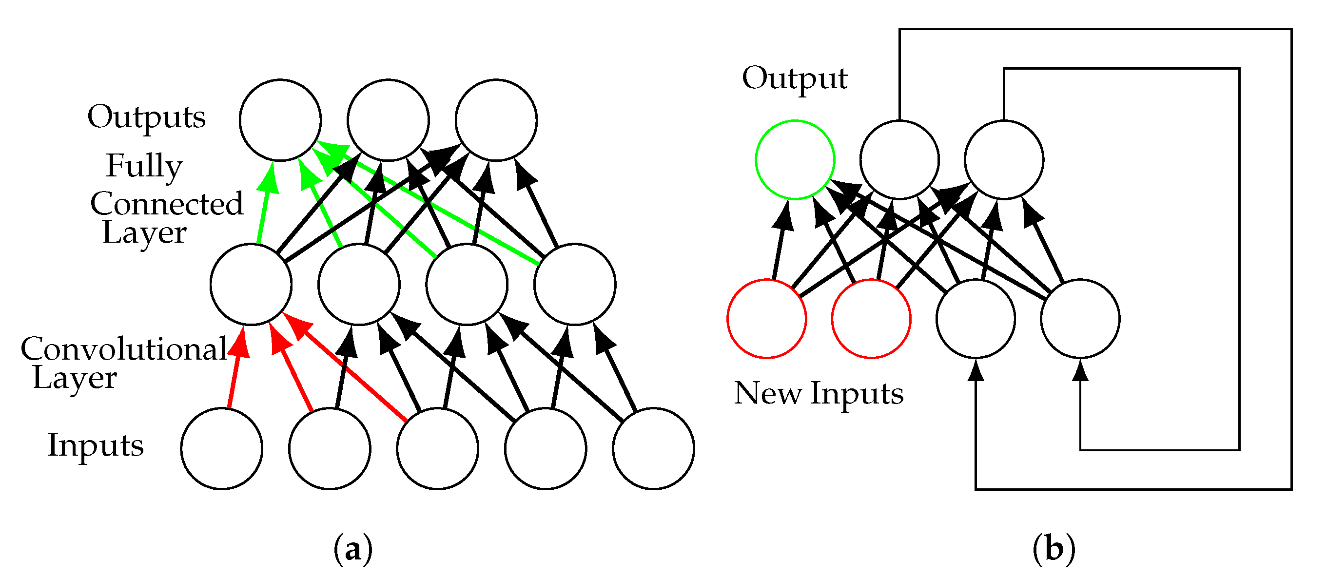
2.3. Deep Neural Network Architectures
3. Challenge: Data Quality
3.1. Data Augmentation
3.1.1. Manual Methods
3.1.2. Signal-Processing-Based Methods
3.1.3. Machine-Learning-Based Methods
3.2. Semi-Supervised Learning
3.2.1. Self-Teaching
3.2.2. Generative Models
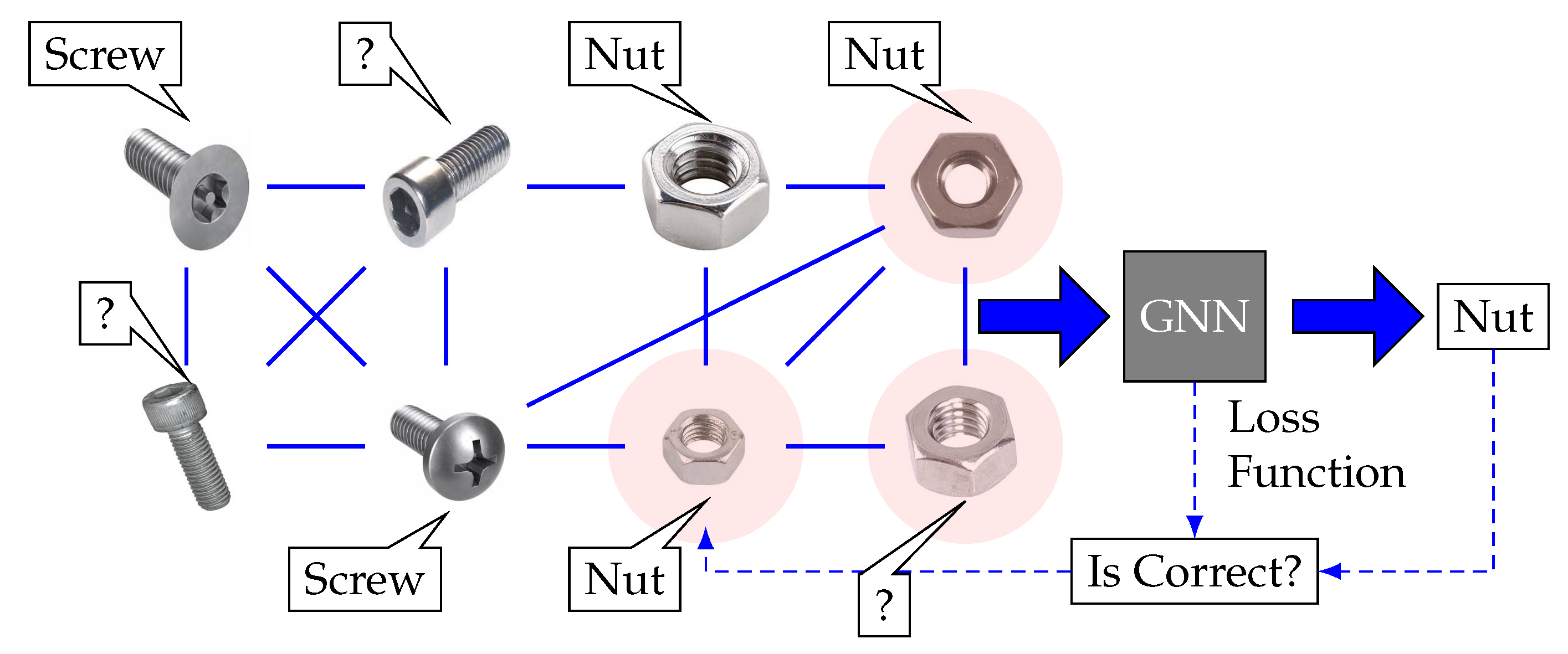
3.2.3. Graph-Based Methods
3.3. Active Learning
3.3.1. Uncertainty Sampling
3.3.2. Diversity Sampling
3.4. Transfer Learning
3.4.1. Instance-Based Transfer Learning
3.4.2. Feature-Based Transfer Learning
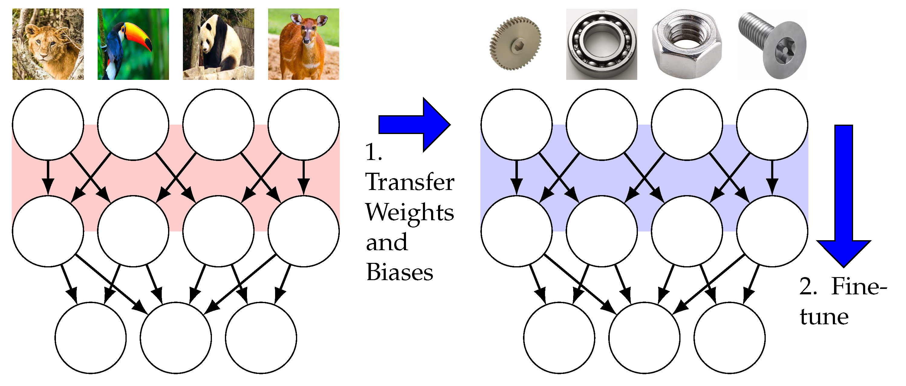
3.4.3. Parameter-Based Transfer Learning
3.5. Continual Learning
3.5.1. Regularization-Based Continual Learning
3.5.2. Memory Reply
3.5.3. Dynamic Architectures
4. Challenge: Data Secrecy
4.1. Elimination Approaches
4.2. Cryptographic Approaches
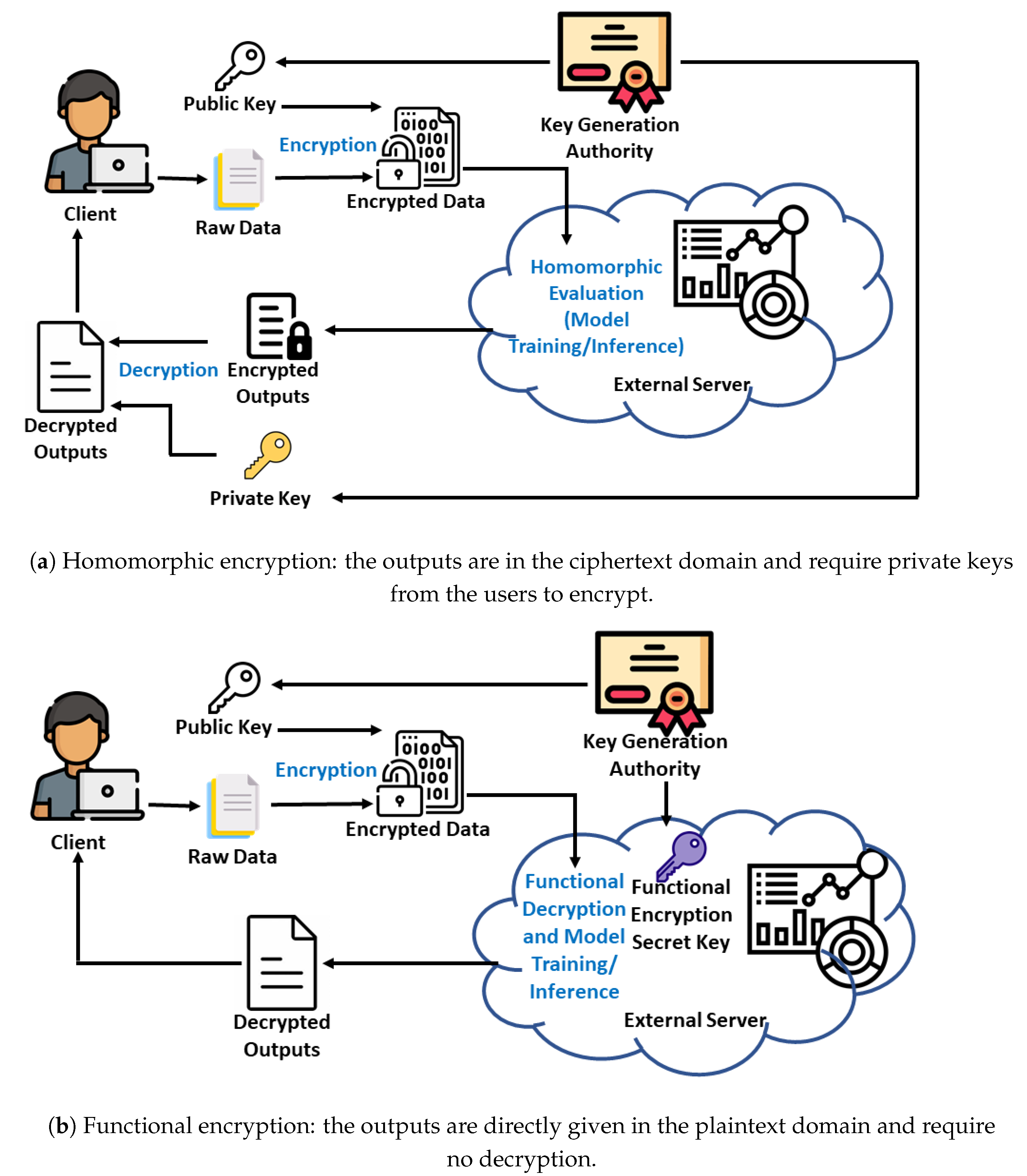
4.2.1. Homomorphic Encryption
4.2.2. Functional Encryption
4.3. Differential Privacy
4.3.1. Data Noising
4.3.2. Gradient Noising
4.4. Federated Learning
5. Challenge: DNN Reliability
5.1. Concept Drift Detection
5.2. Uncertainty Estimation
5.3. Out-of-Distribution Detection
6. Conclusions Trends

| Application Domains | ||||||
|---|---|---|---|---|---|---|
| Challenges | Algorithms | Quality Assurance | Equipment Maintenance | Yield Enhancement | Collaborative Robots | Supply Chain Management |
| Data Augmentation | [64] | [63,66] | [159] | [160] | [161] | |
| Semi-supervised Learning | [5,6,72] | [8] | [11] | [15] | [162] | |
| Data Quality | Active Learning | [82,163] | [78] | – | [164] | – |
| Transfer Learning | [9,10] | [165,166] | [12] | [167] | [168] | |
| Continual Learning | [169,170] | [171] | [13] | [14] | [172] | |
| Cryptographic Approaches | – | [131,173] | – | [174,175] | [176] | |
| Data Secrecy | Differential Privacy | – | [173] | – | [133] | [177] |
| Federated Learning | [178] | [131,179] | – | [133,180] | [181] | |
| Concept Drift Detection | [140,182] | [141,142] | – | [183] | – | |
| DNN Reliability | Uncertainty Estimation | [184,185] | [78,144,145,147] | [186,187] | [188,189] | [190] |
| Out of Distribution Detection | – | [152] | – | – | – | |
Funding
Institutional Review Board Statement
Informed Consent Statement
Data Availability Statement
Conflicts of Interest
References
- Silver, D.; Huang, A.; Maddison, C.J.; Guez, A.; Sifre, L.; Van Den Driessche, G.; Schrittwieser, J.; Antonoglou, I.; Panneershelvam, V.; Lanctot, M.; et al. Mastering the Game of Go with Deep neural Networks and Tree Search. Nature 2016, 529, 484–489. [Google Scholar] [CrossRef] [PubMed]
- Google. Cloud Vision API. Available online: https://cloud.google.com/vision (accessed on 18 July 2022).
- Research, D. AI Enablement on the Way to Smart Manufacturing: Deloitte Survey on AI Adoption in Manufacturing; Technical Report; Deloitte: London, UK, 2020. [Google Scholar]
- Ellström, M.; Erwin, T.; Ringland, K.; Lulla, S. AI in European Manufacturing Industries 2020; Technical Report; Microsoft: Redmond, WA, USA, 2020. [Google Scholar]
- Zheng, X.; Wang, H.; Chen, J.; Kong, Y.; Zheng, S. A Generic Semi-Supervised Deep Learning-Based Approach for Automated Surface Inspection. IEEE Access 2020, 8, 114088–114099. [Google Scholar] [CrossRef]
- Di, H.; Ke, X.; Peng, Z.; Zhou, D. Surface Defect Classification of Steels with a New Semi-Supervised Learning Method. Opt. Lasers Eng. 2019, 117, 40–48. [Google Scholar] [CrossRef]
- Zhao, R.; Yan, R.; Wang, J.; Mao, K. Learning to Monitor Machine Health with Convolutional Bi-Directional LSTM Networks. Sensors 2017, 17, 273. [Google Scholar] [CrossRef] [PubMed]
- Yoon, A.S.; Lee, T.; Lim, Y.; Jung, D.; Kang, P.; Kim, D.; Park, K.; Choi, Y. Semi-Supervised Learning with Deep Generative Models for Asset Failure Prediction. arXiv 2017, arXiv:1709.00845. [Google Scholar]
- Mittel, D.; Kerber, F. Vision-Based Crack Detection using Transfer Learning in Metal Forming Processes. In Proceedings of the 24th International Conference on Emerging Technologies and Factory Automation (ETFA’19), Zaragoza, Spain, 10–13 September 2019; pp. 544–551. [Google Scholar]
- Alencastre-Miranda, M.; Johnson, R.R.; Krebs, H.I. Convolutional Neural Networks and Transfer Learning for Quality Inspection of Different Sugarcane Varieties. IEEE Trans. Ind. Inform. 2020, 17, 787–794. [Google Scholar] [CrossRef]
- Kong, Y.; Ni, D. A Semi-Supervised and Incremental Modeling Framework for Wafer Map Classification. IEEE Trans. Semicond. Manuf. 2020, 33, 62–71. [Google Scholar] [CrossRef]
- Imoto, K.; Nakai, T.; Ike, T.; Haruki, K.; Sato, Y. A CNN-Based Transfer Learning Method for Defect Classification in Semiconductor Manufacturing. In Proceedings of the International Symposium on Semiconductor Manufacturing (ISSM’18), Tokyo, Japan, 10–11 December 2018; pp. 1–3. [Google Scholar]
- Zhang, X.; Zou, Y.; Li, S. Enhancing Incremental Deep Learning for FCCU End-Point Quality Prediction. Inf. Sci. 2020, 530, 95–107. [Google Scholar] [CrossRef]
- Alambeigi, F.; Wang, Z.; Hegeman, R.; Liu, Y.H.; Armand, M. A Robust Data-Driven Approach for Online Learning and Manipulation of Unmodeled 3-D Heterogeneous Compliant Objects. IEEE Trans. Robot. Autom. 2018, 3, 4140–4147. [Google Scholar] [CrossRef]
- Bynum, J. A Semi-Supervised Machine Learning Approach for Acoustic Monitoring of Robotic Manufacturing Facilities. Ph.D. Dissertation, George Mason University, Fairfax, VA, USA, 2020. [Google Scholar]
- Mrazovic, P.; Larriba-Pey, J.L.; Matskin, M. A Deep Learning Approach for Estimating Inventory Rebalancing Demand in Bicycle Sharing Systems. In Proceedings of the 42nd Annual Computer Software and Applications Conference (COMPSAC’18), Tokyo, Japan, 23–27 July 2018; Volume 2, pp. 110–115. [Google Scholar]
- Cavalcante, I.M.; Frazzon, E.M.; Forcellini, F.A.; Ivanov, D. A Supervised Machine Learning Approach to Data-Driven Simulation of Resilient Supplier Selection in Digital Manufacturing. Int. J. Inf. Manag. 2019, 49, 86–97. [Google Scholar] [CrossRef]
- Li, Y.; Chu, F.; Feng, C.; Chu, C.; Zhou, M. Integrated Production Inventory Routing Planning for Intelligent Food Logistics Systems. IEEE Trans. Intell. Transp. Syst. 2018, 20, 867–878. [Google Scholar] [CrossRef]
- Woschank, M.; Rauch, E.; Zsifkovits, H. A Review of Further Directions for Artificial Intelligence, Machine Learning, and Deep Learning in Smart Logistics. Sustainability 2020, 12, 3760. [Google Scholar] [CrossRef]
- Ran, Y.; Zhou, X.; Lin, P.; Wen, Y.; Deng, R. A Survey of Predictive Maintenance: Systems, Purposes and Approaches. arXiv 2019, arXiv:1912.07383. [Google Scholar]
- Lwakatare, L.E.; Raj, A.; Crnkovic, I.; Bosch, J.; Olsson, H.H. Large-scale Machine Learning Systems in Real-World Industrial Settings: A Review of Challenges and Solutions. Inf. Softw. Technol. 2020, 127, 106368. [Google Scholar] [CrossRef]
- Hernavs, J.; Ficko, M.; Berus, L.; Rudolf, R.; Klančnik, S. Deep Learning in Industry 4.0—Brief Overview. J. Prod. Eng 2018, 21, 1–5. [Google Scholar] [CrossRef]
- Wang, J.; Ma, Y.; Zhang, L.; Gao, R.X.; Wu, D. Deep Learning for Smart Manufacturing: Methods and Applications. J. Manuf. Syst. 2018, 48, 144–156. [Google Scholar] [CrossRef]
- Shang, C.; You, F. Data Analytics and Machine Learning for Smart Process Manufacturing: Recent Advances and Perspectives in the Big Data Era. Engineering 2019, 5, 1010–1016. [Google Scholar] [CrossRef]
- Bertolini, M.; Mezzogori, D.; Neroni, M.; Zammori, F. Machine Learning for Industrial Applications: A Comprehensive Literature Review. Expert Syst. Appl. 2021, 175, 114820. [Google Scholar] [CrossRef]
- Dogan, A.; Birant, D. Machine Learning and Data Mining in Manufacturing. Expert Syst. Appl. 2021, 166, 114060. [Google Scholar] [CrossRef]
- Sharp, M.; Ak, R.; Hedberg, T., Jr. A Survey of the Advancing Use and Development of Machine Learning in Smart Manufacturing. J. Manuf. Syst. 2018, 48, 170–179. [Google Scholar] [CrossRef]
- Kim, D.H.; Kim, T.J.; Wang, X.; Kim, M.; Quan, Y.J.; Oh, J.W.; Min, S.H.; Kim, H.; Bhandari, B.; Yang, I.; et al. Smart Machining Process using Machine Learning: A Review and Perspective on Machining Industry. Int. J. Precis. Eng. Manuf.-Green Technol. 2018, 5, 555–568. [Google Scholar] [CrossRef]
- Çınar, Z.M.; Abdussalam Nuhu, A.; Zeeshan, Q.; Korhan, O.; Asmael, M.; Safaei, B. Machine Learning in Predictive Maintenance towards Sustainable Smart Manufacturing in Industry 4.0. Sustainability 2020, 12, 8211. [Google Scholar] [CrossRef]
- Nasir, V.; Sassani, F. A Review on Deep Learning in Machining and Tool Monitoring: Methods, Opportunities, and Challenges. Int. J. Adv. Manuf. Technol. 2021, 115, 2683–2709. [Google Scholar] [CrossRef]
- Weichert, D.; Link, P.; Stoll, A.; Rüping, S.; Ihlenfeldt, S.; Wrobel, S. A Review of Machine Learning for the Optimization of Production Processes. Int. J. Adv. Manuf. Technol. 2019, 104, 1889–1902. [Google Scholar] [CrossRef]
- Wang, C.; Tan, X.; Tor, S.; Lim, C. Machine learning in additive manufacturing: State-of-the-art and perspectives. Addit. Manuf. 2020, 36, 101538. [Google Scholar] [CrossRef]
- Yang, J.; Li, S.; Wang, Z.; Dong, H.; Wang, J.; Tang, S. Using Deep Learning to Detect Defects in Manufacturing: A Comprehensive Survey and Current Challenges. Materials 2020, 13, 5755. [Google Scholar] [CrossRef]
- Kotsiopoulos, T.; Sarigiannidis, P.; Ioannidis, D.; Tzovaras, D. Machine Learning and Deep Learning in Smart Manufacturing: The Smart Grid Paradigm. Comput. Sci. Rev. 2021, 40, 100341. [Google Scholar] [CrossRef]
- Wang, F.; Zhang, M.; Wang, X.; Ma, X.; Liu, J. Deep Learning for Edge Computing Applications: A State-of-the-art Survey. IEEE Access 2020, 8, 58322–58336. [Google Scholar] [CrossRef]
- Ma, X.; Yao, T.; Hu, M.; Dong, Y.; Liu, W.; Wang, F.; Liu, J. A Survey on Deep Learning Empowered IoT Applications. IEEE Access 2019, 7, 181721–181732. [Google Scholar] [CrossRef]
- Ng, A. Machine Learning. Available online: https://www.coursera.org/learn/machine-learning (accessed on 8 August 2021).
- Nwankpa, C.; Ijomah, W.; Gachagan, A.; Marshall, S. Activation Functions: Comparison of Trends in Practice and Research for Deep Learning. arXiv 2018, arXiv:1811.03378. [Google Scholar]
- Chen, T.; Chen, H.; Liu, R.w. Approximation Capability in C (R/sup n/) by Multilayer Feedforward Networks and Related Problems. IEEE Trans. Neural Netw. 1995, 6, 25–30. [Google Scholar] [CrossRef] [PubMed]
- Deng, L. A Tutorial Survey of Architectures, Algorithms, and Applications for Deep Learning. APSIPA Trans. Signal Inf. Process. 2014, 3. [Google Scholar] [CrossRef]
- Bengio, Y. Learning Deep Architectures for AI; Now Publishers Inc.: Delft, The Netherlands, 2009. [Google Scholar]
- Krizhevsky, A.; Sutskever, I.; Hinton, G.E. Imagenet Classification with Deep Convolutional Neural Networks. In Proceedings of the 26th Annual Conference on Neural Information Processing Systems (NIPS’12), Lake Tahoe, NV, USA, 5–10 December 2013; pp. 1097–1105. [Google Scholar]
- Lipton, Z.C.; Berkowitz, J.; Elkan, C. A Critical Review of Recurrent Neural Networks for Sequence Learning. arXiv arXiv:1506.00019, 2015.
- Nanduri, A.; Sherry, L. Anomaly Detection in Aircraft Data using Recurrent Neural Networks (RNN). In Proceedings of the 12th International Conference on Networking and Services (ICNS’16), Lisbon, Portugal, 26–30 June 2016; p. 5C2-1. [Google Scholar]
- Kingma, D.P.; Welling, M. Auto-Encoding Variational Bayes. In Proceedings of the 1st International Conference on Learning Representations (ICLR’13), Scottsdale, AZ, USA, 2–4 May 2013; OpenReview: Scottsdale, AZ, USA, 2013. [Google Scholar]
- Dzmitry, B.; Kyunghyun, C.; Yoshua, B. Neural Machine Translation by Jointly Learning to Align and Translate. In Proceedings of the 3rd International Conference on Learning Representations (ICLR’15), San Diego, CA, USA, 7–9 May 2015; OpenReview: San Diego, CA, USA, 2015. [Google Scholar]
- Li, Y.; Yang, Y.; Zhu, K.; Zhang, J. Clothing Sale Forecasting by a Composite GRU–Prophet Model With an Attention Mechanism. IEEE Trans. Ind. Inform. 2021, 17, 8335–8344. [Google Scholar] [CrossRef]
- Wang, Y.; Deng, L.; Zheng, L.; Gao, R.X. Temporal Convolutional Network with Soft Thresholding and Attention Mechanism for Machinery Prognostics. J. Manuf. Syst. 2021, 60, 512–526. [Google Scholar] [CrossRef]
- van Veen, F. The Neural Network Zoo. Available online: https://www.asimovinstitute.org/neural-network-zoo/ (accessed on 10 August 2021).
- Kadar, M.; Onita, D. A deep CNN for image analytics in automated manufacturing process control. In Proceedings of the 2019 11th International Conference on Electronics, Computers and Artificial Intelligence (ECAI’19), Pitesti, Romania, 27–29 June 2019. [Google Scholar]
- Wei, P.; Liu, C.; Liu, M.; Gao, Y.; Liu, H. CNN-based reference comparison method for classifying bare PCB defects. J. Eng. 2018, 2018, 1528–1533. [Google Scholar] [CrossRef]
- Curreri, F.; Patanè, L.; Xibilia, M.G. RNN-and LSTM-based soft sensors transferability for an industrial process. Sensors 2021, 21, 823. [Google Scholar] [CrossRef]
- Khan, A.H.; Li, S.; Luo, X. Obstacle avoidance and tracking control of redundant robotic manipulator: An RNN-based metaheuristic approach. IEEE Trans. Ind. Inform. 2019, 16, 4670–4680. [Google Scholar] [CrossRef]
- Nguyen, H.; Tran, K.P.; Thomassey, S.; Hamad, M. Forecasting and Anomaly Detection approaches using LSTM and LSTM Autoencoder techniques with the applications in supply chain management. Int. J. Inf. Manag. 2021, 57, 102282. [Google Scholar] [CrossRef]
- Yun, H.; Kim, H.; Jeong, Y.H.; Jun, M.B. Autoencoder-based anomaly detection of industrial robot arm using stethoscope based internal sound sensor. J. Intell. Manuf. 2021, 1–18. [Google Scholar] [CrossRef]
- Tsai, D.M.; Jen, P.H. Autoencoder-based anomaly detection for surface defect inspection. Adv. Eng. Inform. 2021, 48, 101272. [Google Scholar] [CrossRef]
- Liu, C.; Tang, D.; Zhu, H.; Nie, Q. A novel predictive maintenance method based on deep adversarial learning in the intelligent manufacturing system. IEEE Access 2021, 9, 49557–49575. [Google Scholar] [CrossRef]
- Wu, Y.; Dai, H.N.; Tang, H. Graph neural networks for anomaly detection in industrial internet of things. IEEE Internet Things J. 2021, 9, 9214–9231. [Google Scholar] [CrossRef]
- Cooper, C.; Zhang, J.; Gao, R.X.; Wang, P.; Ragai, I. Anomaly detection in milling tools using acoustic signals and generative adversarial networks. Procedia Manuf. 2020, 48, 372–378. [Google Scholar] [CrossRef]
- Liu, H.; Liu, Z.; Jia, W.; Lin, X.; Zhang, S. A novel transformer-based neural network model for tool wear estimation. Meas. Sci. Technol. 2020, 31, 065106. [Google Scholar] [CrossRef]
- Shorten, C.; Khoshgoftaar, T.M. A Survey on Image Data Augmentation for Deep Learning. J. Big Data 2019, 6, 60. [Google Scholar] [CrossRef]
- Arcidiacono, C.S. An Empirical Study on Synthetic Image Generation Techniques for Object Detectors. 2018. Available online: http://www.diva-portal.se/smash/get/diva2:1251485/FULLTEXT01.pdf (accessed on 10 August 2021).
- Lessmeier, C.; Kimotho, J.; Zimmer, D.; Sextro, W. Condition Monitoring of Bearing Damage in Electromechanical Drive Systems by Using Motor Current Signals of Electric Motors: A Benchmark Data Set for Data-Driven Classification. Available online: https://mb.uni-paderborn.de/en/kat/main-research/datacenter/bearing-datacenter/data-sets-and-download/ (accessed on 10 August 2021).
- Cui, W.; Zhang, Y.; Zhang, X.; Li, L.; Liou, F. Metal Additive Manufacturing Parts Inspection Using Convolutional Neural Network. Appl. Sci. 2020, 10, 545. [Google Scholar] [CrossRef]
- Gao, J.; Song, X.; Wen, Q.; Wang, P.; Sun, L.; Xu, H. RobustTAD: Robust Time Series Anomaly Detection via Decomposition and Convolutional Neural Networks. arXiv 2020, arXiv:2002.09545. [Google Scholar]
- Gao, X.; Deng, F.; Yue, X. Data Augmentation in Fault Diagnosis based on the Wasserstein Generative Adversarial Network with Gradient Penalty. Neurocomputing 2019, 396, 487–494. [Google Scholar] [CrossRef]
- Bird, J.J.; Faria, D.R.; Ekárt, A.; Ayrosa, P.P. From Simulation to Reality: CNN Transfer Learning for Scene Classification. In Proceedings of the 10th International Conference on Intelligent Systems (IS’18), Varna, Bulgaria, 28–30 August 2020. [Google Scholar]
- Chapelle, O.; Scholkopf, B.; Zien, A. Semi-Supervised Learning. IEEE Trans. Neural Netw. 2009, 20, 542. [Google Scholar] [CrossRef]
- Lee, D.H. Pseudo-label: The Simple and Efficient Semi-Supervised Learning Method for Deep Neural Networks. In Proceedings of the Workshop on Challenges in Representation Learning, ICML 2013, Atlanta, GA, USA, 16–21 June 2013; Volume 3. [Google Scholar]
- Rajani, C.; Klami, A.; Salmi, A.; Rauhala, T.; Hæggström, E.; Myllymäki, P. Detecting Industrial Fouling by Monotonicity During Ultrasonic Cleaning. In Proceedings of the International Workshop on Machine Learning for Signal Processing (MLSP’18), Aalborg, Denmark, 17–20 September 2018; pp. 1–6. [Google Scholar]
- Kingma, D.P.; Mohamed, S.; Rezende, D.J.; Welling, M. Semi-Supervised Learning with Deep Generative Models. In Proceedings of the Advances in Neural Information Processing Systems (NIPS’14), Montréal, QC, Canada, 8–13 December 2014; pp. 3581–3589. [Google Scholar]
- Zhang, S.; Ye, F.; Wang, B.; Habetler, T.G. Semi-Supervised Learning of Bearing Anomaly Detection via Deep Variational Autoencoders. arXiv 2019, arXiv:1912.01096. [Google Scholar]
- Yang, Z.; Cohen, W.; Salakhudinov, R. Revisiting Semi-Supervised Learning with Graph Embeddings. In Proceedings of the International Conference on Machine Learning (ICML’16), New York, NY, USA, 19–24 June 2016; pp. 40–48. [Google Scholar]
- Chen, C.; Liu, Y.; Kumar, M.; Qin, J.; Ren, Y. Energy Consumption Modelling using Deep Learning Embedded Semi-Supervised Learning. Comput. Ind. Eng. 2019, 135, 757–765. [Google Scholar] [CrossRef]
- Jospin, L.V.; Buntine, W.L.; Boussaid, F.; Laga, H.; Bennamoun, M. Hands-on Bayesian Neural Networks—A Tutorial for Deep Learning Users. arXiv 2018, arXiv:2007.06823. [Google Scholar] [CrossRef]
- Houlsby, N.; Huszár, F.; Ghahramani, Z.; Lengyel, M. Bayesian active learning for classification and preference learning. arXiv 2018, arXiv:1112.5745. [Google Scholar]
- Kirsch, A.; Van Amersfoort, J.; Gal, Y. Batchbald: Efficient and diverse batch acquisition for deep bayesian active learning. In Proceedings of the 33rd Conference Neural Information Processing Systems (NIPS’19), Vancouver, BC, Canada, 8–14 December 2019; Volume 32, pp. 7026–7037. [Google Scholar]
- Martínez-Arellano, G.; Ratchev, S. Towards An Active Learning Approach To Tool Condition Monitoring With Bayesian Deep Learning. In Proceedings of the ECMS 2019, Caserta, Italy, 11–14 June 2019; pp. 223–229. [Google Scholar]
- Geifman, Y.; El-Yaniv, R. Deep Active Learning over the Long Tail. arXiv 2017, arXiv:1711.00941. [Google Scholar]
- Sener, O.; Savarese, S. Active Learning for Convolutional Neural Networks: A Core-Set Approach. In Proceedings of the International Conference Neural Information Processing Systems (ICLR’18), Siem Reap, Cambodia, 13–16 December 2018; ACM: Vancouver, BC, Canada, 2018. [Google Scholar]
- Chen, J.; Zhou, D.; Guo, Z.; Lin, J.; Lyu, C.; Lu, C. An Active Learning Method based on Uncertainty and Complexity for Gearbox Fault Diagnosis. IEEE Access 2019, 7, 9022–9031. [Google Scholar] [CrossRef]
- Xu, Z.; Liu, J.; Luo, X.; Zhang, T. Cross-Version Defect Prediction via Hybrid Active Learning with Kernel Principal Component Analysis. In Proceedings of the 25th International Conference on Software Analysis, Evolution and Reengineering (SANER’18), Campobasso, Italy, 20–23 March 2018. [Google Scholar]
- Pan, S.J.; Yang, Q. A Survey on Transfer Learning. IEEE Trans. Knowl. Data Eng 2009, 22, 1345–1359. [Google Scholar] [CrossRef]
- Perdana, R.S.; Ishida, Y. Instance-Based Deep Transfer Learning on Cross-domain Image Captioning. In Proceedings of the International Electronics Symposium (IES’2019), Surabaya, Indonesia, 27–28 September 2019; pp. 24–30. [Google Scholar]
- Wang, B.; Qiu, M.; Wang, X.; Li, Y.; Gong, Y.; Zeng, X.; Huang, J.; Zheng, B.; Cai, D.; Zhou, J. A Minmax Game for Instance-based Selective Transfer Learning. In Proceedings of the 25th International Conference on Knowledge Discovery and Data Mining (KDD’19), Anchorage, AK, USA, 4–8 August 2019; pp. 34–43. [Google Scholar]
- Zhang, L.; Guo, L.; Gao, H.; Dong, D.; Fu, G.; Hong, X. Instance-based Ensemble Deep Transfer Learning Network: A New Intelligent Degradation Recognition Method and Its Application on Ball Screw. Mech. Syst. Signal Process. 2020, 140, 106681. [Google Scholar] [CrossRef]
- Long, M.; Wang, J. Learning Multiple Tasks with Deep Relationship Networks. In Proceedings of the 31st Conference on Neural Information Processing Systems (NIPS’17), Long Beach, CA, USA, 4–9 December 2017; pp. 1593–1602. [Google Scholar]
- Zhu, J.; Chen, N.; Shen, C. A New Deep Transfer Learning Method for Bearing Fault Diagnosis under Different Working Conditions. IEEE Sens. J. 2019, 20, 8394–8402. [Google Scholar] [CrossRef]
- Kim, S.; Kim, W.; Noh, Y.K.; Park, F.C. Transfer Learning for Automated Optical Inspection. In Proceedings of the International Joint Conference on Neural Networks (IJCNN’17), Anchorage, AK, USA, 14–19 May 2017; pp. 2517–2524. [Google Scholar]
- Krizhevsky, A. Learning Multiple Layers of Features from Tiny Images. 2009. Available online: https://www.cs.toronto.edu/~kriz/learning-features-2009-TR.pdf (accessed on 20 September 2021).
- Weiaicunzai. Awesome—Image Classification. Available online: https://github.com/weiaicunzai/awesome-image-classification (accessed on 20 September 2021).
- Parisi, G.I.; Kemker, R.; Part, J.L.; Kanan, C.; Wermter, S. Continual Lifelong Learning with Neural Networks: A Review. Neural Netw. 2019, 113, 54–71. [Google Scholar] [CrossRef]
- Zenke, F.; Poole, B.; Ganguli, S. Continual Learning through Synaptic Intelligence. In Proceedings of the 34th International Conference on Machine Learning (ICML’17), Sydney, Australia, 6–11 August 2017; pp. 3987–3995. [Google Scholar]
- Li, Z.; Hoiem, D. Learning without Forgetting. IEEE Trans. Pattern Anal. Mach. Intell. 2017, 40, 2935–2947. [Google Scholar] [CrossRef] [PubMed]
- Li, D.; Tasci, S.; Ghosh, S.; Zhu, J.; Zhang, J.; Heck, L. RILOD: Near Real-Time Incremental Learning for Object Detection at the Edge. In Proceedings of the 4th Symposium on Edge Computing (SEC’19), Arlington, VA, USA, 7–9 November 2019; pp. 113–126. [Google Scholar]
- De Lange, M.; Aljundi, R.; Masana, M.; Parisot, S.; Jia, X.; Leonardis, A.; Slabaugh, G.; Tuytelaars, T. Continual Learning: A Comparative Study on How to Defy Forgetting in Classification Tasks. arXiv 2019, arXiv:1909.08383. [Google Scholar]
- Lopez-Paz, D.; Ranzato, M. Gradient Episodic Memory for Continual Learning. In Proceedings of the 31st Conference on Neural Information Processing Systems (NIPS’17), Long Beach, CA, USA, 4–9 December 2017; pp. 6467–6476. [Google Scholar]
- Shin, H.; Lee, J.K.; Kim, J.; Kim, J. Continual Learning with Deep Generative Replay. In Proceedings of the 31st Conference on Neural Information Processing Systems (NIPS’17), Long Beach, CA, USA, 4–9 December 2017; pp. 2990–2999. [Google Scholar]
- Wiewel, F.; Yang, B. Continual Learning for Anomaly Detection with Variational Autoencoder. In Proceedings of the 44th International Conference on Acoustics, Speech and Signal Processing (ICASSP’19), Brighton, UK, 12–17 May 2019; pp. 3837–3841. [Google Scholar]
- Mallya, A.; Lazebnik, S. Packnet: Adding Multiple Tasks to A Single Network by Iterative Pruning. In Proceedings of the 34th Conference on Computer Vision and Pattern Recognition (CVPR’18), Salt Lake City, UT, USA, 18–22 June 2018; pp. 7765–7773. [Google Scholar]
- Rusu, A.A.; Rabinowitz, N.C.; Desjardins, G.; Soyer, H.; Kirkpatrick, J.; Kavukcuoglu, K.; Pascanu, R.; Hadsell, R. Progressive Neural Networks. arXiv 2016, arXiv:1606.04671. [Google Scholar]
- Castro, F.M.; Marín-Jiménez, M.J.; Guil, N.; Schmid, C.; Alahari, K. End-to-End Incremental Learning. In Proceedings of the 15th European Conference on Computer Vision (ECCV’18), Munich, Germany, 8–14 September 2018; pp. 233–248. [Google Scholar]
- Tuptuk, N.; Hailes, S. Security of Smart Manufacturing Systems. J. Manuf. Syst. 2018, 47, 93–106. [Google Scholar] [CrossRef]
- Samarati, P.; Sweeney, L. Protecting Privacy when Disclosing Information: K-anonymity and its Enforcement through Generalization and Suppression. In Proceedings of the IEEE Symposium on Research in Security and Privacy (S&P), Oakland, CA, USA, 3–6 May 1998. [Google Scholar]
- Machanavajjhala, A.; Kifer, D.; Gehrke, J.; Venkitasubramaniam, M. L-diversity: Privacy beyond K-anonymity. ACM Trans. Knowl. Discov. Data (TKDD) 2007, 1, 3-es. [Google Scholar] [CrossRef]
- Li, N.; Li, T.; Venkatasubramanian, S. t-Closeness: Privacy Beyond k-Anonymity and l-Diversity. In Proceedings of the 2007 IEEE 23rd International Conference on Data Engineering (ICDE’13), Istanbul, Turkey, 15–20 April 2007. [Google Scholar]
- Meden, B.; Emeršič, Ž.; Štruc, V.; Peer, P. K-Same-Net: K-Anonymity with Generative Deep Neural Networks for Face Deidentification. Entropy 2018, 20, 60. [Google Scholar] [CrossRef]
- Gentry, C. Fully Homomorphic Encryption using Ideal Lattices. In Proceedings of the 41st Annual Symposium on Theory of Computing (STOC’09), Washington, DC, USA, 31 May–2 June 2009; pp. 169–178. [Google Scholar]
- Zhang, Q.; Yang, L.T.; Chen, Z. Privacy Preserving Deep Computation Model on Cloud for Big Data Feature Learning. IEEE Trans. Comput. 2015, 65, 1351–1362. [Google Scholar] [CrossRef]
- Gilad-Bachrach, R.; Dowlin, N.; Laine, K.; Lauter, K.; Naehrig, M.; Wernsing, J. Cryptonets: Applying Neural Networks to Encrypted Data with High Throughput and Accuracy. In Proceedings of the International Conference on Machine Learning (ICML’16), New York, NY, USA, 20–22 June 2016; pp. 201–210. [Google Scholar]
- Azure. Enterprise Security and Governance for Azure Machine Learning. Available online: https://docs.microsoft.com/en-us/azure/security/fundamentals/encryption-overview (accessed on 12 November 2021).
- Meng, X. Machine Learning Models that Act on Encrypted Data. Available online: https://www.amazon.science/blog/machine-learning-models-that-act-on-encrypted-data (accessed on 12 November 2021).
- Zhu, L.; Tang, X.; Shen, M.; Gao, F.; Zhang, J.; Du, X. Privacy-Preserving Machine Learning Training in IoT Aggregation Scenarios. IEEE Internet Things J. 2021, 8, 12106–12118. [Google Scholar] [CrossRef]
- Ryffel, T.; Dufour-Sans, E.; Gay, R.; Bach, F.; Pointcheval, D. Partially Encrypted Machine Learning using Functional Encryption. In Proceedings of the 33rd Conference Neural Information Processing Systems (NIPS’19), Vancouver, BC, Canada, 8–14 December 2019. [Google Scholar]
- Abdalla, M.; Bourse, F.; Caro, A.D.; Pointcheval, D. Simple Functional Encryption Schemes for Inner Products. In Proceedings of the IACR International Workshop on Public Key Cryptography, Gaithersburg, MD, USA, 30 March–1 April 2015; pp. 733–751. [Google Scholar]
- Boneh, D.; Franklin, M. Identity-based Encryption from the Weil Pairing. In Proceedings of the Annual International Cryptology Conference (CRYPTO’01), Santa Barbara, CA, USA, 19–23 August 2001; pp. 213–229. [Google Scholar]
- Xu, R.; Joshi, J.B.; Li, C. Cryptonn: Training Neural Networks over Encrypted Data. In Proceedings of the 39th International Conference on Distributed Computing Systems (ICDCS’19), Dallas, TX, USA, 7–9 July 2019; pp. 1199–1209. [Google Scholar]
- Chrysos, G.G.; Moschoglou, S.; Bouritsas, G.; Deng, J.; Panagakis, Y.; Zafeiriou, S.P. Deep Polynomial Neural Networks. IEEE Trans. Pattern Anal. Mach. Intell. 2021, 44, 4021–4034. [Google Scholar] [CrossRef]
- Song, Q.; Cao, J.; Sun, K.; Li, Q.; Xu, K. Try before You Buy: Privacy-preserving Data Evaluation on Cloud-based Machine Learning Data Marketplace. In Proceedings of the Annual Computer Security Applications Conference (ACSAC’21), Austin, TX, USA, 6–10 December 2021; pp. 260–272. [Google Scholar]
- Dwork, C.; Roth, A. The Algorithmic Foundations of Differential Privacy. Found. Trends Theor. Comput. Sci. 2014, 9, 3–4. [Google Scholar]
- Kenthapadi, K.; Mironov, I.; Thakurta, A.G. Privacy-preserving data mining in industry. In Proceedings of the WSDM 2019, Melbourne, Australia, 11–15 February 2019; pp. 840–841. [Google Scholar]
- Huang, C.; Kairouz, P.; Chen, X.; Sankar, L.; Rajagopal, R. Context-aware generative adversarial privacy. Entropy 2017, 19, 656. [Google Scholar] [CrossRef]
- Kopp, A. Microsoft Smartnoise Differential Privacy Machine Learning Case Studies; Microsoft Azure White Papers; Microsoft Corporation: Redmond, WA, USA, 2021. [Google Scholar]
- Wu, J.; Dang, Y.; Jia, H.; Liu, X.; Lv, Z. Prediction of Energy Consumption in Digital Twins of Intelligent Factory by Artificial Intelligence. In Proceedings of the 2021 International Conference on Technology and Policy in Energy and Electric Power (ICT-PEP’21), Yogyakarta, Indonesia, 29–30 September 2021; pp. 354–359. [Google Scholar]
- Abadi, M.; Chu, A.; Goodfellow, I.; McMahan, H.B.; Mironov, I.; Talwar, K.; Zhang, L. Deep Learning with Differential Privacy. In Proceedings of the Conference on Computer and Communications Security (SIGSAC’16), Vienna, Austria, 24–28 October 2016; pp. 308–318. [Google Scholar]
- Papernot, N.; Song, S.; Mironov, I.; Raghunathan, A.; Talwar, K.; Erlingsson, U. Scalable Private Learning with PATE. In Proceedings of the 6st International Conference on Learning Representations (ICLR’18), Vancouver, BC, Canada, 30 April–3 May 2018. [Google Scholar]
- Gong, M.; Xie, Y.; Pan, K.; Feng, K.; Qin, A.K. A Survey on Differentially Private Machine Learning. IEEE Comput. Intell. Mag. 2020, 15, 49–64. [Google Scholar] [CrossRef]
- Konečnỳ, J.; McMahan, H.B.; Yu, F.X.; Richtárik, P.; Suresh, A.T.; Bacon, D. Federated learning: Strategies for Improving Communication Efficiency. arXiv 2016, arXiv:1610.05492. [Google Scholar]
- Chen, M.; Yang, Z.; Saad, W.; Yin, C.; Poor, H.V.; Cui, S. A Joint Learning and Communications Framework for Federated Learning over Wireless Networks. arXiv 2020, arXiv:1909.07972. [Google Scholar] [CrossRef]
- Hao, M.; Li, H.; Luo, X.; Xu, G.; Yang, H.; Liu, S. Efficient and Privacy-Enhanced Federated Learning for Industrial Artificial Intelligence. IEEE Trans. Ind. Inform. 2019, 16, 6532–6542. [Google Scholar] [CrossRef]
- Bagheri, B.; Rezapoor, M.; Lee, J. A Unified Data Security Framework for Federated Prognostics and Health Management in Smart Manufacturing. Manuf. Lett. 2020, 24, 136–139. [Google Scholar] [CrossRef]
- Wei, K.; Li, J.; Ding, M.; Ma, C.; Yang, H.H.; Farokhi, F.; Jin, S.; Quek, T.Q.; Poor, H.V. Federated Learning with Differential Privacy: Algorithms and Performance Analysis. IEEE Trans. Inf. Forensics Secur. 2020, 15, 3454–3469. [Google Scholar] [CrossRef]
- Zhou, W.; Li, Y.; Chen, S.; Ding, B. Real-Time Data Processing Architecture for Multi-Robots Based on Differential Federated Learning. In Proceedings of the SmartWorld/SCALCOM/UIC/ATC/CBDCom/IOP/SCI 2018, Guangzhou, China, 8–12 October 2018; pp. 462–471. [Google Scholar]
- Vepakomma, P.; Gupta, O.; Swedish, T.; Raskar, R. Split Learning for Health: Distributed Deep Learning without Sharing Raw Patient Data. arXiv 2018, arXiv:1812.00564. [Google Scholar]
- Abuadbba, S.; Kim, K.; Kim, M.; Thapa, C.; Camtepe, S.A.; Gao, Y.; Kim, H.; Nepal, S. Can We Use Split Learning on 1D CNN Models for Privacy Preserving Training? arXiv 2020, arXiv:2003.12365. [Google Scholar]
- Saria, S.; Subbaswamy, A. Tutorial: Safe and Reliable Machine Learning. arXiv 2019, arXiv:1904.07204. [Google Scholar]
- Ren, P.; Xiao, Y.; Chang, X.; Huang, P.Y.; Li, Z.; Chen, X.; Wang, X. A Comprehensive Survey of Neural Architecture Search: Challenges and Solutions. ACM Comput. Surv. (CSUR) 2021, 54, 1–34. [Google Scholar] [CrossRef]
- Dreyfus, P.A.; Pélissier, A.; Psarommatis, F.; Kiritsis, D. Data-based Model Maintenance in the Era of Industry 4.0: A Methodology. J. Manuf. Syst. 2022, 63, 304–316. [Google Scholar] [CrossRef]
- Lu, J.; Liu, A.; Dong, F.; Gu, F.; Gama, J.; Zhang, G. Learning under Concept Drift: A Review. IEEE Trans. Knowl. Data Eng. 2018, 31, 2346–2363. [Google Scholar] [CrossRef]
- Kabir, M.A.; Keung, J.W.; Bennin, K.E.; Zhang, M. Assessing the Significant Impact of Concept Drift in Software Defect Prediction. In Proceedings of the 43rd Annual Computer Software and Applications Conference (COMPSAC’19), Milwaukee, WI, USA, 15–19 July 2019; Volume 1, pp. 53–58. [Google Scholar] [CrossRef]
- Zenisek, J.; Holzinger, F.; Affenzeller, M. Machine Learning-based Concept Drift Detection for Predictive Maintenance. Comput. Ind. Eng. 2019, 137, 106031. [Google Scholar] [CrossRef]
- Bermeo-Ayerbe, M.A.; Ocampo-Martinez, C.; Diaz-Rozo, J. Data-driven Energy Prediction Modeling for Both Energy Efficiency and Maintenance in Smart Manufacturing Systems. Energy 2022, 238, 121691. [Google Scholar] [CrossRef]
- Gal, Y. Uncertainty in Deep Learning. Ph.D. Dissertation, Cambridge University, Cambridge, UK, 2016. [Google Scholar]
- Peng, W.; Ye, Z.S.; Chen, N. Bayesian Deep-Learning-Based Health Prognostics Toward Prognostics Uncertainty. IEEE Trans. Ind. Electron. 2019, 67, 2283–2293. [Google Scholar] [CrossRef]
- Benker, M.; Furtner, L.; Semm, T.; Zaeh, M.F. Utilizing uncertainty Information in Remaining Useful Life Estimation via Bayesian Neural Networks and Hamiltonian Monte Carlo. J. Manuf. Syst. 2021, 61, 799–807. [Google Scholar] [CrossRef]
- Lakshminarayanan, B.; Pritzel, A.; Blundell, C. Simple and Scalable Predictive Uncertainty Estimation using Deep Ensembles. In Proceedings of the 31st Conference on Neural Information Processing Systems (NIPS’17), Long Beach, CA, USA, 4–9 December 2017; pp. 6402–6413. [Google Scholar]
- Nemani, V.P.; Lu, H.; Thelen, A.; Hu, C.; Zimmerman, A.T. Ensembles of Probabilistic LSTM Predictors and Correctors for Bearing Prognostics using Industrial Standards. Neurocomputing 2022, 491, 575–596. [Google Scholar] [CrossRef]
- DeVries, T.; Taylor, G.W. Learning Confidence for Out-of-distribution Detection in Neural Networks. arXiv 2018, arXiv:1802.04865. [Google Scholar]
- Hendrycks, D.; Gimpel, K. A Baseline for Detecting Misclassified and Out-of-distribution Examples in Neural Networks. In Proceedings of the 7th International Conference Neural Information Processing Systems (ICLR’18), Montréal, ON, Canada, 3–8 December 2018; OpenReview: San Juan, Puerto Rico, 2018. [Google Scholar]
- Lee, K.; Lee, K.; Lee, H.; Shin, J. A Simple Unified Framework for Detecting Out-of-distribution Samples and Adversarial Attacks. In Proceedings of the 32rd Conference on Neural Information Processing Systems (NIPS’18), Montreal, QC, Canada, 3–8 December 2018; pp. 7167–7177. [Google Scholar]
- Bendale, A.; Boult, T.E. Towards Open Set Deep Networks. In Proceedings of the 32nd International Conference on Computer Vision and Pattern Recognition (CVPR’16), Las Vegas, NV, USA, 27–30 June 2016; pp. 1563–1572. [Google Scholar]
- Xu, J.; Kovatsch, M.; Lucia, S. Open Set Recognition for Machinery Fault Diagnosis. In Proceedings of the 19st International Conference on Industrial Informatics (INDIN’21), Palma de Mallorca, Spain, 21–23 July 2021; pp. 1–7. [Google Scholar]
- Berthelot, D.; Roelofs, R.; Sohn, K.; Carlini, N.; Kurakin, A. AdaMatch: A Unified Approach to Semi-Supervised Learning and Domain Adaptation. In Proceedings of the 9th International Conference on Learning Representations (ICLR’21), Online, 3–7 May 2021. [Google Scholar]
- Wang, Y.; Gu, Q.; Brown, D. Differentially Private Hypothesis Transfer Learning. In Proceedings of the European Conference on Machine Learning and Principles and Practice of Knowledge Discovery in Databases (ECML-PKDD’18), Dublin, Ireland, 10–14 September 2018; pp. 811–826. [Google Scholar]
- Farrall, F.; Mittal, N.; Narra, C.; Tello, J.; Dow, E.M. Data-Sharing Made Easy; Technical Report; Deloitte: London, UK, 2021. [Google Scholar]
- Otto, B.; Mohr, N.; Roggendorf, M.; Guggenberger, T. Data Sharing in Industrial Ecosystems; Technical Report; McKinsey: New York, NY, USA, 2020. [Google Scholar]
- Pandey, A.V. Future of AI in Business: Adaptive Machine Learning Models That Evolve and Improve over Time without Expensive Retraining. Available online: https://www.nvidia.com/en-us/on-demand/session/gtcfall20-a21421/ (accessed on 24 November 2021).
- Cattaneo, G.; Vanara, F.; Massaro, A. Advanced Technologies for Industry—AT WATCH echnology Focus on Cloud Computing; Technical Report; EU Commission: Brussels, Belgium, 2020. [Google Scholar]
- Nakazawa, T.; Kulkarni, D.V. Wafer Map Defect Pattern Classification and Image Retrieval using Convolutional Neural Network. IEEE Trans. Semicond. Manuf. 2019, 31, 309–314. [Google Scholar] [CrossRef]
- Labbé, Y.; Carpentier, J.; Aubry, M.; Sivic, J. Single-view Robot Pose and Joint Angle Estimation via Render and Compare. arXiv 2021, arXiv:2104.09359. [Google Scholar]
- Priore, P.; Ponte, B.; Rosillo, R.; de la Fuente, D. Applying Machine Learning to the Dynamic Selection of Replenishment Policies in Fast-changing Supply Chain Environments. Int. J. Prod. Res. 2018, 57, 3663–3677. [Google Scholar] [CrossRef]
- Liu, F.; Zhong, D. GSOS-ELM: An RFID-Based Indoor Localization System Using GSO Method and Semi-Supervised Online Sequential ELM. Sensors 2018, 18, 1995. [Google Scholar] [CrossRef]
- Bellini, M.; Pantalos, G.; Kaspar, P.; Knoll, L.; De-Michielis, L. An Active Deep Learning Method for the Detection of Defects in Power Semiconductors. In Proceedings of the 32nd Annual SEMI Advanced Semiconductor Manufacturing Conference (ASMC’21), Milpitas, CA, USA, 10–12 May 2021. [Google Scholar]
- Wilde, N.; Kulić, D.; Smith, S.L. Bayesian Active Learning for Collaborative Task Specification using Equivalence Regions. IEEE Robot. Autom. Lett. 2019, 4, 1691–1698. [Google Scholar] [CrossRef]
- Ma, P.; Zhang, H.; Fan, W.; Wang, C.; Wen, G.; Zhang, X. A Novel Bearing Fault Diagnosis Method Based on 2D Image Representation and Transfer Learning Convolutional Neural Network. Meas. Sci. Technol. 2019, 30, 055402. [Google Scholar] [CrossRef]
- Xiao, D.; Huang, Y.; Zhao, L.; Qin, C.; Shi, H.; Liu, C. Domain Adaptive Motor Fault Diagnosis using Deep Transfer Learning. IEEE Access 2019, 7, 80937–80949. [Google Scholar] [CrossRef]
- Cai, J.; Zhang, Z.; Cheng, H. Grasping Novel Objects by Semi-supervised Domain Adaptation. In Proceedings of the Conference on Real-Time Computing and Robotics (RCAR’19), Irkutsk, Russia, 4–9 August 2019; pp. 626–631. [Google Scholar]
- Nguyen, T.T.; Hatua, A.; Sung, A.H. Cumulative Training and Transfer Learning for Multi-Robots Collision-Free Navigation Problems. In Proceedings of the 10th Annual Ubiquitous Computing, Electronics & Mobile Communication Conference (UEMCON’19), New York, NY, USA, 10–12 October 2019; pp. 305–311. [Google Scholar]
- Oh, Y.; Ransikarbum, K.; Busogi, M.; Kwon, D.; Kim, N. Adaptive SVM-based Real-time Quality Assessment for Primer-sealer Dispensing Process of Sunroof Assembly Line. Reliab. Eng. Syst. Saf. 2019, 184, 202–212. [Google Scholar] [CrossRef]
- Mera, C.; Orozco-Alzate, M.; Branch, J. Incremental Learning of Concept Drift in Multiple Instance Learning for Industrial Visual Inspection. Comput. Ind. 2019, 109, 153–164. [Google Scholar] [CrossRef]
- Yu, W.; Zhao, C. Broad Convolutional Neural Network-based Industrial Process Fault Diagnosis with Incremental Learning Capability. IEEE Trans. Ind. Electron. 2019, 67, 5081–5091. [Google Scholar] [CrossRef]
- Raj, A.; Majumder, A.; Kumar, S. HiFI: A Hierarchical Framework for Incremental Learning using Deep Feature Representation. In Proceedings of the 28th International Conference on Robot and Human Interactive Communication (RO-MAN’19), New Delhi, India, 14–18 October 2019; pp. 1–6. [Google Scholar]
- Kong, Q.; Lu, R.; Yin, F.; Cui, S. Privacy-Preserving Continuous Data Collection for Predictive Maintenance in Vehicular Fog-Cloud. IEEE Trans. Intell. Transp. Syst. 2020, 22, 5060–5070. [Google Scholar] [CrossRef]
- Chen, Y.; Ping, Y.; Zhang, Z.; Wang, B.; He, S. Privacy-preserving Image Multi-classification Deep Learning Model in Robot System of Industrial IoT. Neural Comput. Appl. 2021, 33, 4677–4694. [Google Scholar] [CrossRef]
- Chen, Y.; Wang, B.; Zhang, Z. PDLHR: Privacy-Preserving Deep Learning Model with Homomorphic Re-Encryption in Robot System. IEEE Syst. J. 2021. [Google Scholar] [CrossRef]
- Khan, P.W.; Byun, Y.C.; Park, N. IoT-Blockchain Enabled Optimized Provenance System for Food Industry 4.0 Using Advanced Deep Learning. Sensors 2020, 20, 2990. [Google Scholar] [CrossRef] [PubMed]
- Zheng, X.; Cai, Z. Privacy-preserved data sharing towards multiple parties in industrial IoTs. IEEE J. Sel. Areas Commun. 2020, 38, 968–979. [Google Scholar] [CrossRef]
- Han, X.; Yu, H.; Gu, H. Visual Inspection with Federated Learning. In Proceedings of the 16th International Conference on Image Analysis and Recognition (ICIAR’19), Waterloo, ON, Canada, 27–29 August 2019; pp. 52–64. [Google Scholar]
- Kanagavelu, R.; Li, Z.; Samsudin, J.; Yang, Y.; Yang, F.; Goh, R.S.M.; Cheah, M.; Wiwatphonthana, P.; Akkarajitsakul, K.; Wangz, S. Two-Phase Multi-Party Computation Enabled Privacy-Preserving Federated Learning. arXiv 2020, arXiv:2005.11901. [Google Scholar]
- Lim, H.K.; Kim, J.B.; Heo, J.S.; Han, Y.H. Federated Reinforcement Learning for Training Control Policies on Multiple IoT Devices. Sensors 2020, 20, 1359. [Google Scholar] [CrossRef]
- Yin, F.; Lin, Z.; Xu, Y.; Kong, Q.; Li, D.; Theodoridis, S. FedLoc: Federated Learning Framework for Cooperative Localization and Location Data Processing. arXiv 2020, arXiv:2003.03697. [Google Scholar] [CrossRef]
- Diez-Olivan, A.; Ortego, P.; Del Ser, J.; Landa-Torres, I.; Galar, D.; Camacho, D.; Sierra, B. Adaptive Dendritic Cell-deep Learning Approach for Industrial Prognosis under Changing Conditions. IEEE Trans. Ind. Inform. 2021, 17, 7760–7770. [Google Scholar] [CrossRef]
- Maisenbacher, M.; Weidlich, M. Handling Concept Drift in Predictive Process Monitoring. SCC 2017, 17, 1–8. [Google Scholar]
- Sajedi, S.O.; Liang, X. Uncertainty-assisted Deep Vision Structural Health Monitoring. Comput.-Aided Civ. Infrastruct. Eng. 2020, 36, 126–142. [Google Scholar] [CrossRef]
- Li, Y.T.; Kuo, P.; Guo, J.I. Automatic Industry PCB Board DIP Process Defect Detection with Deep Ensemble Method. In Proceedings of the 29th International Symposium on Industrial Electronics (ISIE’20), Delft, The Netherlands, 17–19 June 2020; pp. 453–459. [Google Scholar]
- Godefroy, G.; Arnal, B.; Bossy, E. Compensating for Visibility Artefacts in Photoacoustic Imaging with A Deep Learning Approach Providing Prediction Uncertainties. Photoacoustics 2020, 21, 100218. [Google Scholar] [CrossRef] [PubMed]
- Lu, Y.; Wang, Z.; Xie, R.; Liang, S. Bayesian Optimized Deep Convolutional Network for Electrochemical Drilling Process. J. Manuf. Mater. Process. 2019, 3, 57. [Google Scholar] [CrossRef]
- Thakur, S.; van Hoof, H.; Higuera, J.C.G.; Precup, D.; Meger, D. Uncertainty aware Learning from Demonstrations in Multiple Contexts using Bayesian Neural Networks. In Proceedings of the International Conference on Robotics and Automation (ICRA’19), Montreal, QC, Canada, 20–24 May 2019; pp. 768–774. [Google Scholar]
- Miller, D.; Dayoub, F.; Milford, M.; Sünderhauf, N. Evaluating Merging Strategies for Sampling-based Uncertainty Techniques in Object Detection. In Proceedings of the International Conference on Robotics and Automation (ICRA’19), Montreal, QC, Canada, 20–24 May 2019; pp. 2348–2354. [Google Scholar]
- Mercier, S.; Uysal, I. Neural network models for Predicting perishable Food Temperatures along the Supply Chain. Biosyst. Eng. 2018, 171, 91–100. [Google Scholar] [CrossRef]
| Contents | Survey Articles |
|---|---|
| Deep learning basics and list of use cases | Deep learning in industry 4.0—brief overview [22] |
| Deep learning basics and list of use cases | Deep learning for smart manufacturing: methods and applications [23] |
| Deep learning basics and list of use cases | Data analytics and machine learning for smart process manufacturing: recent advances and perspectives in the big data era [24] |
| Machine learning basics and use case categories in smart manufacturing | Machine Learning for industrial applications: A comprehensive literature review [25] |
| Machine learning basics and use case categories in smart manufacturing | Machine learning and data mining in manufacturing [26] |
| Categorization of machine learning applications in smart manufacturing | A survey of the advancing use and development of machine learning in smart manufacturing [27] |
| Machine learning use cases in machining process | Smart machining process using machine learning: a review and perspective on machining industry [28] |
| Deep learning for predictive maintenance | Machine learning in predictive maintenance towards sustainable smart manufacturing in industry 4.0 [29] |
| Deep learning for predictive maintenance | A survey of predictive maintenance: systems, purposes and approaches [20] |
| Deep learning for machinery tool monitoring | A review on deep learning in machining and tool monitoring: methods, opportunities, and challenges [30] |
| Deep learning for smart logistics | A review of further directions for artificial intelligence, machine learning, and deep learning in smart logistics [19] |
| Deep learning for production process optimization | A review of machine learning for the optimization of production processes [31] |
| Deep learning for additive manufacturing | Machine learning in additive manufacturing: state-of-the-art and perspectives [32] |
| Deep learning for defect detection | Using deep learning to detect defects in manufacturing: a comprehensive survey and current challenges [33] |
| Deep learning for smart grid | Machine learning and deep learning in smart manufacturing: the smart grid paradigm [34] |
| Edge computing for deep learning in smart manufacturing | Deep learning for edge computing applications: a state-of-the-art survey [35] |
| Software development for deep learning in smart manufacturing | Large-scale machine learning systems in real-world industrial settings: a review of challenges and solutions [21] |
| IoT for deep learning in smart manufacturing | A survey on deep learning empowered IoT applications [36] |
| Deep Learning Models | Brief Introduction | Examples |
|---|---|---|
| Convolutional Neural Network (CNN) | Neural networks containing convolutional kernels. Usually used for 2D data, such as visual inspection. | [10,50,51] |
| Recurrent Neural Network (RNN) | Neural networks containing recurrent cells. Usually used for data streams, such as sensory stream data analysis. | [44,52,53] |
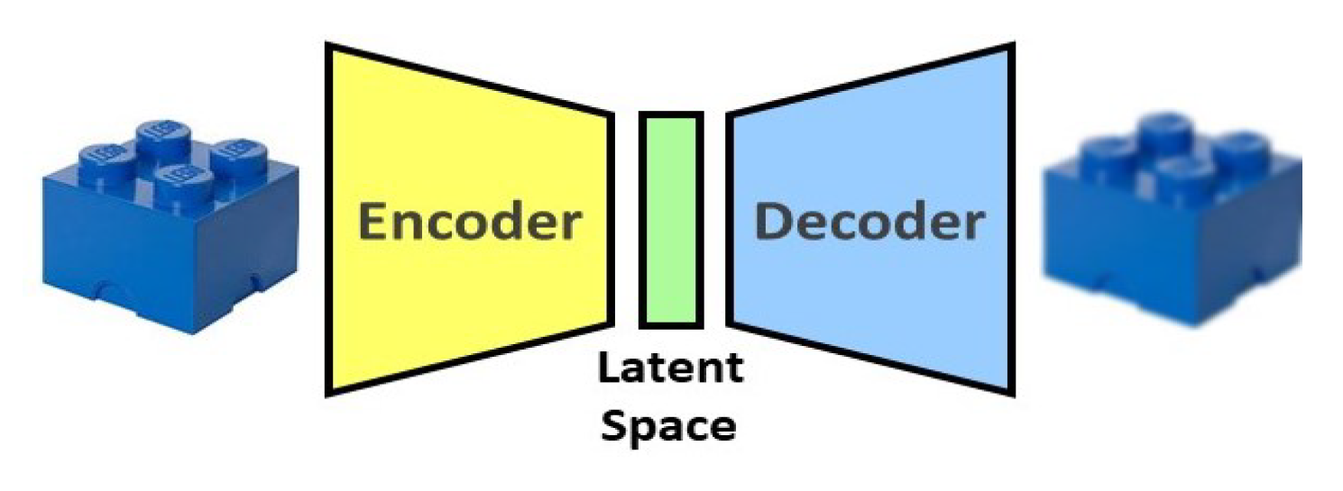
| AutoEncoder (AE) | AEs are usually used for feature extraction since it can learn essential information for data reconstruction. AEs are trained in an unsupervised fashion. | [54,55,56] |
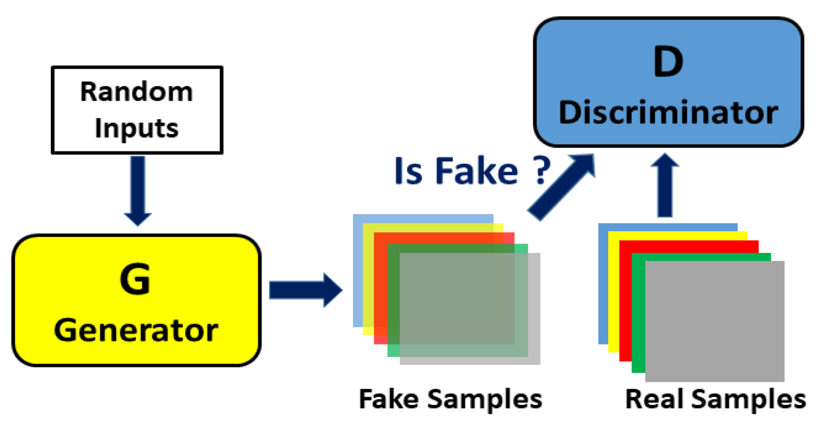
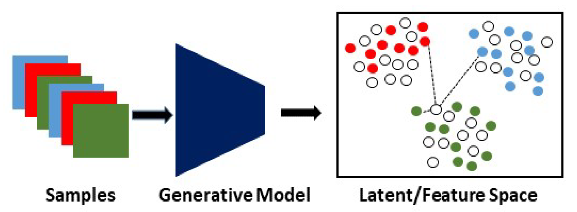
| Generative Adversarial Neural Network (GAN) | GANs can learn the statistical distributions of the training data in an unsupervised way. Therefore, GANs are often used for anomaly detection. | [57,58,59] |
| Transformer | Transformers can learn to differently weight an important part of the inputs. Transformers were originally used for data streams. | [47,48,60] |
| PPML Techniques | Applied Scenarios | Applied Objects |
|---|---|---|
| Elimination-based Approaches | Cloud | Data |
| Homomorphic Encryption | Cloud | Data, Model |
| Functional Encryption | Cloud | Data, Model |
| Differential Privacy | Cloud, Edge | Data, Model |
| Federated Learning | Edge | Architecture |
Publisher’s Note: MDPI stays neutral with regard to jurisdictional claims in published maps and institutional affiliations. |
© 2022 by the authors. Licensee MDPI, Basel, Switzerland. This article is an open access article distributed under the terms and conditions of the Creative Commons Attribution (CC BY) license (https://creativecommons.org/licenses/by/4.0/).
Share and Cite
Xu, J.; Kovatsch, M.; Mattern, D.; Mazza, F.; Harasic, M.; Paschke, A.; Lucia, S. A Review on AI for Smart Manufacturing: Deep Learning Challenges and Solutions. Appl. Sci. 2022, 12, 8239. https://doi.org/10.3390/app12168239
Xu J, Kovatsch M, Mattern D, Mazza F, Harasic M, Paschke A, Lucia S. A Review on AI for Smart Manufacturing: Deep Learning Challenges and Solutions. Applied Sciences. 2022; 12(16):8239. https://doi.org/10.3390/app12168239
Chicago/Turabian StyleXu, Jiawen, Matthias Kovatsch, Denny Mattern, Filippo Mazza, Marko Harasic, Adrian Paschke, and Sergio Lucia. 2022. "A Review on AI for Smart Manufacturing: Deep Learning Challenges and Solutions" Applied Sciences 12, no. 16: 8239. https://doi.org/10.3390/app12168239
APA StyleXu, J., Kovatsch, M., Mattern, D., Mazza, F., Harasic, M., Paschke, A., & Lucia, S. (2022). A Review on AI for Smart Manufacturing: Deep Learning Challenges and Solutions. Applied Sciences, 12(16), 8239. https://doi.org/10.3390/app12168239