Abstract
The length of a spliced pile is 2 m assembled from an original spiral pile using a connector. The whole pile is the structure of the upper straight pipe and the lower spiral. The pile–soil model is established with FEM-SPH by LS-DYNA to simulate and analyze the characteristics of the spliced piles. When the helical pile is subjected to a horizontal load, the pile rotates around the point of rotation, and the contact force position of the soil in the model is as expected. During the process of pile driving, the soil forms an inverted cone stress-area, and the maximum particle stress area near the pile tip and the ground surface is 400 Kpa, which is highly concentrated. When loaded laterally, the area of the interaction stress of the soil particles is divided into three regions: the stress effect region; the transition region; and the critical region. Then, 7° is defined as the ultimate horizontal bearing-capacity of the spliced pile, and the numerical simulation of the horizontal bearing-capacity fundamentally matches the test results. The simulation model realizes the transition from the pile installation to the lateral loading, predicts the ultimate horizontal bearing-capacity, and analyzes the stress distribution of the soil particles and the time-development of the soil displacement.
1. Introduction
A helical pile can be guided to sink to a predetermined depth by transmitting torque through the blades to spin into the soil. Compared to the traditional hammering and static-pressing methods, the spliced helical pile has significant advantages in the form of minor damage to the ground surface, weak vibration, and low noise during the pile-installation process. After the installation, the helical piles are loaded immediately and can be used for dam closure, rope hooking, and the foundations for PV-support brackets [1,2].
In order to accurately research the performance of the piles under lateral load, many scholars have developed pile model testing devices for the X-ray–CT method. In the study by Eskisar [3], X-ray–CT methods were used as a non-destructive technique to quantify the load distribution mechanism. Cui [4] conducted model tests and X-ray–computed tomography analysis to study permeable concrete pile (PCP) blockages. Otani [5] accurately observed the damage pattern of sandy soils under pile lateral loads by performing model loading tests with X-ray–CT scanning. The CT methods are limited to model tests and are expensive. The methods are not always available in most laboratories. Alternatively, there was the use of transparent soil technology visualization to measure the horizontal stressed-soil displacement on the side of the pile, with a non-intrusive capture by particle imagery, overcoming the barriers to measurement caused by the opacity of the natural soil [6,7,8,9,10]. However, this method makes it difficult to simulate the working of full-size piles of soil.
Numerical simulations can be used to obtain results that are similar to the actual ones [11,12,13], and the analysis of the soil model uses a solid mesh-cell approach, where the meshes themselves are already co-noded with each other, which can lead to various difficulties in dealing with free surfaces, deformable boundaries, moving interfaces, large deformations, and crack extensions. In addition, the generation of high-quality meshes is time-consuming for problems involving complex geometry. Hu [14] simulated high-pressure melting, Peng [15] modeled a large landslide, Liu [16,17] achieved excellent results in an underwater explosion, and Cai [18] and Xi [19] used smooth particle hydrodynamics (SPH) methods for the simulation of liquid-swaying flows during shipment. As no meshes are used, the connectivity between the particles is generated as part of the calculation and varies over time. SPH is an adequate replacement for CT image capture and entire 3D displacement-measurement systems for the 3D displacement fields of the soil around the laterally loaded piles in transparent and coastal sandy soils. The soil model of pile–soil interaction uses the SPH approach to simulate the micromechanical behavior of the soil at the minor particle level, including the contact stresses and displacements, to explain phenomena that cannot be directly observed and experimentally discussed. Because of its Lagrangian character, a time history can be obtained, and the free surfaces, material interfaces, and moving boundaries can be easily tracked during simulation by properly deploying the particles at specific locations during the initial phase.
Lv [20] used Ansys to simulate the deformation of welded piles. Pang [21] analyzed the resistance of the sunken pile according to the principle of pile–soil action and the theory of mechanical equilibrium; then, specific measures were proposed to appropriately reduce the outer diameter of the hollow cylinder, while keeping the outer diameter of the base of the cone unchanged and appropriately reducing the length of the helical blade. Hu [22] slotted the pile at the tip and reduced the sinking time by 8.85%. However, the monolithic helical piles are only suitable for specific applications where spliced helical piles are an ideal structure to permit them to continue to operate under different working conditions. However, the horizontal load-bearing of the spliced helical pile has not been studied, especially since the pile structure becomes longer after splicing, which has a significant impact on the lateral load-bearing ability. The interaction between the pile and the soil needs to be further studied.
In this paper, the finite element modeling analysis of soil and spliced piles is carried out using SPH and Lagrangian methods, respectively. The numerical simulations are completed continuously from the sunken pile to the horizontal bearing, and the internal particle time-development processes, stress states, and aggregation can be analyzed during the pile–soil interaction. The ultimate load-carrying capacity of the spliced pile tested by field tests is compared with the simulation to verify the reliability of the simulation model.
2. Numerical Description
Finite Element Analysis is a mathematical method of simulating and approximating actual physical systems for various complex geometric and loading conditions. It is a widely used and effective tool for transforming complex practical problems into simpler ones. This method involves discretizing a complete solution range into a number of elementary units, which are connected at the nodes, and the approximate solution of the problem is subsequently obtained by solving each unit. The Navier–Stokes (NS) equation governs the hydrodynamic problem, which can be written in the following formulation:
In the above equation, , , , denote the density, velocity vector, pressure, gravity, and dynamic viscosity, respectively.
In the particle approximations, the computational domain is discretized with a group of particles. The field functions and their derivatives can be written as:
where is the approximate value of particle ; is the value of associated with particle ; and are the positions of corresponding particles; N is the number of the particles in the support domain; h is the smooth length; is the smoothing function and represents a weighted contribution of particle to particle [23]. By substituting the SPH approximation of the function and its derivative into the N-S equation, the SPH motion equation of the N–S equation can be obtained, as follows:
In SPH, an artificial compressibility technique is often used to model an incompressible flow as a slightly compressible one. The artificial compressibility considers that every theoretically incompressible fluid is actually compressible. Therefore, it is feasible to use a quasi-incompressible equation of state to model the incompressible flow. In this work, the artificial equation of state is:
where is the sound speed of the concerned artificially compressible fluid (e.g., water). Monaghan [24] argued that the relative density variation, , is related to the fluid bulk velocity and sound speed in the following way:
where , , and are the initial density, absolute density variation, fluid bulk velocity, and Mach number, respectively.
I corresponds to a particle, is the stress tensor in the Kelvin model representation, is the velocity tensor, and is the gradient of the kernel function associated with particle evaluated at particle . is an artificial viscosity, usually set by the keyword Control-Bulk-Viscosity or the hourglass card in LS-DYNA.
The additional viscoplastic strain moves the yield surface outwards with time and the yield surface gradually widens with time, which means that the mechanical properties of the soil have gradually changed. The simulation model is used to quantify the viscoplastic behavior of the surrounding soil, allowing for the consideration of the stress paths, and the stress range effects. The displacement and velocity vectors of the soil are extracted in post-processing by an approximation of the kernel functions and the particle discrete domains.
3. Finite Element Simulation
The numerical simulations were carried out using LS-DYNA finite element analysis software to model a spliced helical pile by applying gravity, rotational velocity, and downward velocity to the helical pile to reach a depth of 700 mm (as the diameter of the spiral part of the pile is 90 mm and the diameter of the upper thicker part of the cable is 108 mm, there is a short transition section in the middle, which reaches a height of 700 mm) and then applying a horizontal variable load, with the following purposes:
- (1)
- Study the displacement and ultimate bearing capacity of the spliced pile under the horizontal load;
- (2)
- Analyze the stress state and aggregation of the soil particles.
3.1. Pile–Soil Model
The pile–soil model is based on the following assumptions:
- (1)
- The soil is a uniformly anisotropic ideal elastic-plastic body;
- (2)
- The shear expansion or shear contraction of the soil is not considered;
- (3)
- The spliced helical pile is considered to be a rigid body.
The helical pile (Table 1) consists of four main parts (Figure 1). In actual operation, the helical blades transmit torque to be screwed into the soil, the flange connects the short pile to the upper hanging part of the cable, and the upper flange enables the splicing of longer piles.

Table 1.
Structural parameters of helical pile (unit: mm).
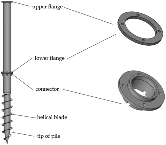
Figure 1.
Structural drawing of spliced helical pile.
The accuracy of the FEM simulations depends mainly on selecting the appropriate material models to represent the soil, structure, and soil–structure interactions. The Q235 is selected as the structural material of the pile, which is set as a rigid body. The outer layer of the soil is fully constrained, and the rigid plate is added at the bottom. The LAGRANGE_IN_SOLID constrains the pile and soil (Table 2). The frame of the pile-sinking hydraulic motor is 40 kg, and the initial loading is 400 N distributed in the upper-end flange. The rotation speed is set at 31.4 m/s, and the descending speed is 0.1 m/s.
Table 2.
Pile and soil material.
3.2. Helical Pile Installation
The original pile takes 1.3 s to sink, and the extended pile takes 1.47 s to sink. The last helical blade is fully inserted into the soil at a depth of 700 mm, and the helical pile is continuously rotated into the soil by shearing the soil with the blade and transmitting torque in the form of counter-thrust. The soil suffers a large plastic deformation. The maximum shear stress reached nearly 400 Kpa, gradually transitioning from 280 Kpa near the pile to zero. The particles in the surface soil layer bulge upwards, and the particles at a depth of 14 mm below the surface layer hold a shear stress of nearly 100 Kpa. The more muscular shear stresses occur mainly in the part of the pile in contact with the surface soil layer, below the soil layer at the locations near the pile body below the surface, and most of the pile tip (Figure 2). The stress areas from 1 to 4 are observed inside the soil layer of the original pile and the stress extends to the boundary until it is zero; the pile tip part interacts strongly with the soil, and the stress is centralized. The rest of the area’s pile–soil interaction is generally due to the blade shearing the soil to guide down the helical pile. The stress area near the pile body is normal.
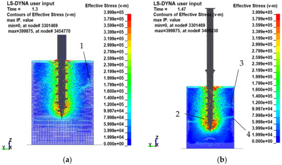
Figure 2.
Finite element simulation of pile–soil installation process: (a) Original pile; (b) Extended pile.
When t = 0.69 s, a wave peak occurs, and the torque is 270.67 N·m (Figure 3). The red area around the pile accumulates, and the soil is severely compressed and stressed. After the wave peak, the consolidated soil is destroyed due to blade shearing, the red area gradually fades, and the torque reaches the maximum value of 669.72 N·m when the stress is reduced. The maximum torque of the original pile was 700.38 N·m at 1.2 s, and the maximum torque of the lengthened pile was 699 N·m at 1.24 s. The results show that the maximum torque required for the lengthened pile and the original pile during the sinking process is the same, and there is no effect on the torque after the lengthening of the structure.
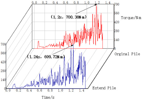
Figure 3.
Output of the time history curves of the extended pile and the original pile in terms of torque.
When additional modifications are required to the keyword file for subsequent dynamic analyses [25], the analysis can be split into two sessions of research. The dynamic file is generated by invoking the *INTERFACE_SPRINGBACK_LSDYNA option [26], and the output corresponds to the dynain file, which corresponds to the position at the end moment of the sunken pile in the first session, as well as to the model cell stress and strain data. The state at the end of the first session of the sunken piles is used as the initial condition for the second session of the lateral loading for stress initialization. When additional models need to be added for import, *INCLUDE and *TRANSFORM can be used to make the appropriate adjustments to the model and keywords [27]. The end state of the spliced pile is retained after the complete sinking of the pile (Figure 2). The state at this point is given a horizontal load of 150 mm below the top of the pile along the x-direction, and the horizontal force is applied to the top of the pile in a gradual linear manner (Figure 2).
The direct effect of the external forces acting on the model is expressed as kinetic and internal energy. At a deficient speed, the kinetic energy can be negligible compared to the internal energy. Therefore, when using this method for stress initialization, the preloading time should be relatively long to minimize the inertial force and the kinetic energy, and to avoid interfering with the subsequent dynamic analysis [28]. The initial stresses at the end of the sunken pile are the initial stresses for lateral loading, taking into account the effect of the spliced pile installation under this model, based on which the pile–soil interaction can be more realistically analyzed (Figure 2).
3.3. Lateral Loading
A full constraint is considered for the bottom of the soil model geometry. For the vertical boundaries on the sides of the model geometry, the full constraint is also required. For the subsurface, the model boundary is considered free in all of the directions. Node number 2941052, to which a tension of 10,000 N is applied (within 0–0.4 s, the direction parallel to the X-axis positive and C (Figure 4) is used as a reference position for the spliced pile), using the keyword *LOAD_NODE_SET to constrain all of the degrees of freedom outside the -axis. It is applied to the spliced pile 150 mm below the top of the pile (Figure 4), with a specified rotation angle of 7°, at which point the stresses are close to the boundary, and the displacement and load of the spliced pile at this point are recorded as the ultimate bearing capacity. The particles in the region 0–60 mm at the surface are gradually approaching the boundary, which consists mainly of the soil particles dominated by the no-action–effect area, where the stresses between the particles are disrupted due to the soil bulge, which is more relaxed and does not have a practical effect on the pile–soil action. The soil particles below 60 mm on the surface do not extend to the boundary. This part of the particles is compacted to form the soil resistance, which carries the main horizontal bearing capacity and prevents the pile from overturning. The internal pile–soil interaction is overall more in accordance with the actual effect.
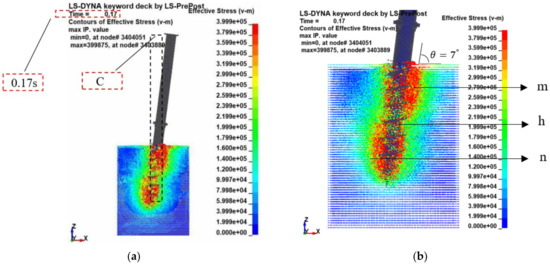
Figure 4.
(a) Relative reference position of pile top displacement; (b) Area of influence of pile–soil action and specified angle.
The stress area of the pile is more centralized, mainly to the left of the pile tip; near to the right side of the pile body, there appears a higher stress area. This can be interpreted as a pivot point lever model, the helical pile with the area as the pivot point (Figure 4), driving the pile body below to rotate, and a violent compression with the soil. However, a secondary offset region of the soil can be found inside, where the soil rotates in the area, creating a greater slip surface on the and pile sides, with a longitudinal slip surface length of 314 mm (approx. 3.5 D pile diameter) for the of the extended pile, 43 mm for the , and 343 mm for the . The delineated lengths are based on the red high-stress areas in both and , and is where the red high-stress area dissipates. It can be seen that the longer length of the original pile area means that the area of the soil slip surface in this area is more extensive, and the soil resistance generated by the soil particles is greater. Although the length of the area elongated pile is higher than the original pile, the most important thing is that the deflection of the area causes the displacement of the soil in the area, so when the pile is carrying horizontally, the horizontal load causes the helical pile to rotate and drive the sliding surface of the soil in the area, the size of the sliding surface directly affects the horizontal bearing capacity of the pile.
The initial loading tension is minor if the helical pile is not constrained to rotate in the direction. In the actual simulation, both the extension pile and the original pile have a slight fluctuation at the beginning of the loading. The lateral load is not enough to cause the helical pile to move horizontally, and the helical pile is unstable in force and starts to rotate in the axial direction. The pile will rotate along the -axis, and only when the loading tension is higher will it move positively on the -axis. Therefore, the displacement should be determined by comparing the end-state pile and the reference position of the whole pile. The displacement of the top of the pile in the central axis of the reference position is measured, and the whole loading process of the two piles (Figure 5).
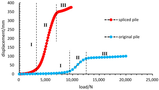
Figure 5.
Load-displacement relationship curve of helical pile under lateral load.
The displacement of both of the piles rises exponentially with the load within the limits of the plastic region of the soil, I for the initial loading region, II for the plastic region, and III for the soil stiffness enhancement region. The pile driving can cause significant perturbation to the surrounding soil and change the soil stress state. The excess pore water pressure will resist the external load with the soil particles at I and dissipate at II, where the soil will exhibit viscoplasticity, and the displacement will show a steady upward trend. As the stresses in the soil extend to the boundary in III, the region of the effect of the pile–soil interaction gradually approaches the boundary, the soil is further compacted, the strength and stiffness of the surrounding soil increase with the increasing load, and the pile displacement in this region grows slowly and reaches the ultimate load-carrying capacity of this simulation model. As 7° is specified as the ultimate load-carrying capacity for the deflection angle of the helical pile, the displacement of the original pile is 25.2 mm, and the load is 10,000 N. The displacement of the spliced pile is 40.27 mm, and the load is 3625 N, both within II, which does not influence the values obtained for the results.
The displacement–soil resistance is based on the pile–soil stresses in the active and passive regions under horizontal tension (Figure 6). The two piles are loaded with a relatively dense number of fetching points at the beginning of the loading. With increasing loads, the displacements are smaller, but the soil resistance has reached higher values, the soil is squeezed dense and gradually reaches the soil’s primary stiffness stability value. The soil particles will experience stable viscoplasticity, with a greater increase in the displacement and smoother curves, corresponding to I and II (Figure 6). After that, the slope of the soil resistance changes, and the displacement grows slowly. This is due to the soil particles being squeezed and the soil displacement region having reached the boundary, while the high-stress region is approaching the boundary of the soil model and the soil reaches a stable value of secondary stiffness. The secondary stiffness arises because the soil model is small, but the number of cells in the whole pile–soil model have reached 500,000, and the simulation is more time-consuming; thus, the boundary effects have an impact on the soil, but the main object of the study is within the area of primary stiffness. The tilt angle and displacement are minor and do not affect the analysis of the pile soil.
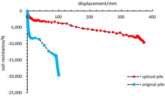
Figure 6.
Soil resistance analysis of pile–soil internal interactions.
4. Soil Internal Analysis
The pile installation process is considered to be cylindrical shear, and the range of soil pressure changes caused by the pile is considered to be lateral resistance; Qiu divided the area of pile–soil influence into three boundaries, based on 0.5 P0 and 0.2 P0, which are named as the no influence region, the critical region, and the effect region, respectively [29]. The lateral loading of the pile–soil action also has a zoning situation, with 7° as the last moment end state (Figure 7). The high-stress region of the elongated pile is the 70 mm effect zone, 110 mm is the transition zone, and 150 mm is the critical zone, with the stress region between the particles showing varying degrees of aggregation, with the particles 60 mm below the surface of the shallow soil layer gradually decreasing to zero from 400 kpa to 140 kpa. It shows that the internal energy at the areas 1 and 2 are significantly higher than elsewhere. The higher internal energy indicates that the pile–soil compression in these two areas is severe and that the particles will experience a greater displacement. It is a direct indication that the helical pile, when subjected to lateral loading, is guided to the left of the pile tip, due to the positive X-axis driving force applied.
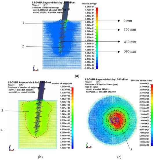
Figure 7.
(a) Internal energy of soil particles; (b) Number of soil particle zones; (c) pile–soil interaction partition.
The areas three and four indicate a step-change in the number of particles in two areas, with the three areas near the pile having a higher degree of compactness, due to the direct interaction between the helical pile and the soil (Figure 7), with aggregation of up to 150 particles, the final state of which is likely to be a significant increase in soil stiffness for the soil. The area at four resulted from the force transfer near the pile, the number of particles crossed and clustered in quantities ranging from 86 to 121, the squeeze was relatively weakened, and a conical area was formed. Most of the particles in the other areas did not receive a more significant squeeze and remained at the original number of 50, modeled by themselves. The quantity cloud reflects more visually the distribution of the soil particles after the pile–soil interaction, followed by an analysis of the displacement of the soil particles from the sensitive areas.
The 5 are on the side of the pile (Figure 7), based on the ground surface as a reference for the particle displacements (Figure 8) of different height positions, with the particles near the pivot point becoming progressively greater in displacement under the horizontal loading in a relatively orderly manner, reflecting the time-varying process of the soil particles during the loading process. The particle displacements of 40 mm and 120 mm appear in the opposite direction, the surface of the pile is curved (Figure 8), the actual force on the particle is vectorial in direction, moving towards a less stressful region, and the soil is gradually compacted and moves within the primary stiffness, resulting in a squeeze back. However, the displacement continues to grow after the force has stabilized. The peak is where the particle has reached the stress boundary of the soil and gradually gathers towards the edge, forming a solid wall boundary and reaching the secondary stiffness of the soil. The load is no longer sufficient for the splice to continue to move and eventually stabilizes at a value. The pile tip particles also gradually increase as the load is applied. The particles (Figure 8) are the displacement of the pile tip particles, 550 mm, that appeared to be extruded back and eventually stabilized at a value. This peak is different from the particles on the pile side, as mainly it is the spliced pile that is loaded, the particles on the pile body and pile side are violently extruded and form a center of rotation inside. When the particles squeeze with the pile, the side no longer moves, and the particle at the tip of the pile also stops moving. In fact, the particle on the loaded side of the pile reaches the primary and secondary stiffness.
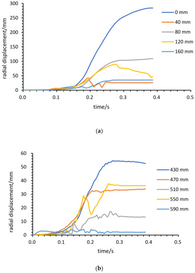
Figure 8.
Spliced pile (a) Pile side; (b) Soil particle displacement at pile tip.
5. Field Test
The tests were conducted on-site for the soils in the Pearl River Basin in Guangzhou and were separated into two parts to execute the test measurements (Figure 9). The first part was a pile installation test on a helical pile, where the strain gauges were attached 70 mm below the top of the pile, and the strain in a pile was transmitted as a voltage signal, via a bridge box, to a digital acquisition oscilloscope recorder. The second session was the horizontal load-bearing test. The tensile pressure transducer loaded the two piles, the piles were deflected, and the displacement of the spliced piles was measured using the reference rod and reference line as the reference position. The piles should be spaced more than ten times the pile diameter, to avoid the overlap of soil stresses on the torque and horizontal load-bearing. Three tests were carried out, respectively, and the data were saved.
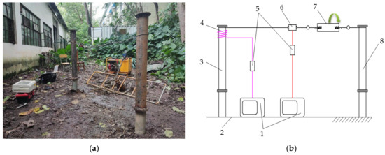
Figure 9.
(a) Field loading test; (b) Test measurement system. 1—Data acquisition system; 2—Sinking pile ground; 3—Spliced pile; 4—Strain gauge and winding wire; 5—Bridge box; 6—Tension sensor; 7—Afterburner; 8—Auxiliary pile.
The maximum strain of 95.91 με in the spliced pile test corresponded to a torque of 666.23 N∙m and a sunken pile depth of 512.5 mm (Figure 10), with a maximum torque of 621.61 N∙m reached at a sunken pile depth of 568.88 mm during the simulation. The spliced pile simulation was a time-development process of the whole pile into the earth, where the larger value of the corresponding moment of the sunken pile torque was taken, and the whole process was more orderly, with a torque error of 6.7% between the simulation and test (Figure 3). The simulation of the initial period of sinking pile had a rising trend, which was due to the pile tip inserting into the soil and the soil extrusion friction, the soil resistance increased, the torque also increased. When the first blade rotated into the soil, there was shallow soil structure destruction, an upward bulge, the blade began to transfer torque to guide the sinking pile body, the pile body and soil extrusion were dense when the blade rotated into the dense area, it started to shear the soil, the slab of soil gradually relaxed, and then thinned. The interaction between the soil and the pile was weakened. The cycle repeated itself, but the overall trend was increasing. During the test, the initial pile tip had already sunk by 160 mm, due to the self-gravity of the spliced pile. The excess pore water pressure, cohesion, and consolidation structures formed in the test were difficult to set in the simulation, resulting in a significantly higher overall test trend than the simulation data.
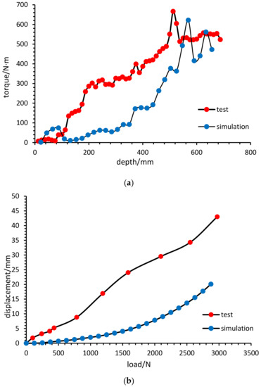
Figure 10.
(a) The pile installation of progress test; (b) Load displacement test of spliced assemblies.
In the lateral bearing capacity test process, two sinking points at a distance of 1500 mm were selected at the base of the sunken pile and sunk into the spliced pile at a standard depth of 700 mm (Figure 10). Two reference rods were embedded in the pile side of the spliced pile, 200 mm away from the pile axis to ensure that the line between the two reference rods passed through the helical pile axis and were perpendicular to the line between the two piles, as a reference for measuring the displacement of the top of the helical pile. During the test, the distance between the two piles was shortened by turning the tightener with a manual lever to measure the displacement of the pile end and the corresponding force. The displacement and the corresponding oscilloscope strain values were recorded every five revolutions of the force tightener. When the spliced pile was deflected by 7°, we waited for the oscilloscope to stabilize and recorded the value, which corresponded to a horizontal load-bearing capacity of 2903 N. The curve rose overall during the loading, and the slope of the curve changed considerably around 1 kN and 2 kN. The soil stiffness gradually increased within the initial 1 kN, due to soil relaxation and the pile squeezing the soil, and after 2 kN, the strength and stiffness of the soil stabilized, and the displacement grew slowly. The overall trend in the simulation was relatively smooth, with an increasing trend during loading, corresponding to a load of 3625 N at 7°, with an error of 24.87%. Compared to the tests, the settings for the clay-plastic soils and stiffness were more idealized, and, since the soil layer was not homogeneous, the actual loading area may have contained debris, slag, etc. The simulation can provide a reference for predicting the horizontal bearing capacity.
6. Conclusions
SPH overcomes the problem of mesh distortion due to large deformations in the numerical simulation, and simulates the time-varying process of the helical pile into the soil by means of smooth particle dynamics. SPH analyses the horizontal bearing characteristics of the spliced pile to the following conclusions:
- (1)
- The horizontal bearing capacity of the screw pile decreases significantly after splicing. The horizontal bearing capacity of the test is 2903 N, and the numerical simulation reaches 3625 N, with an error of 24.87%. The reason for the high error is that the field test environment is challenging to match the simulation, and the soil below the surface contains gravel and residue, which leads to an uneven soil quality. The qualified laboratories can adopt the method of the soil model box, and the soil layer gradient distribution can set more reliable parameters for the established SPH model;
- (2)
- The spliced pile is gradually inclined under the loading of the horizontal force, with 7° as the end state of the ultimate bearing capacity. The soil particles form a more obvious stress aggregation situation on the surface, which can be divided into three regions with the spliced pile as the center, the stress effect zone at 70.25 mm, near the helical blade, the transition zone at 109.81 mm, and the critical zone at 150.37 mm; the SPH particles are relatively independent. The internal visualization of the pile–soil interaction allows for a single analysis of the particles;
- (3)
- The pile–soil model was established in LS-DYNA, perfectly realizing the transition from the pile installation process to the horizontal load bearing. The method of SPH simulated the soil particles at the micro level, showing its unique advantages in pile–soil interaction. From the whole loading process, the soil stiffness changes gradually and finally tends to be stable. The soil under the initial loading is relatively relaxed. With the continuous increase in tension, the soil stiffness shows two apparent changes, and the final displacement increases slowly, reaching the equilibrium state of pile–soil interaction;
- (4)
- The model of SPH can be appropriately expanded so that the soil gradually compacts under the action of the horizontal pulling forces rather than due to the boundary effects. Since the horizontal bearing capacity decreases after splicing, can the structure of the cap base be added to the surface? When the soil parameters are measured outdoors, they can be tested in layers at specified depths and added to established SPH models. Since the SPH model is time-consuming, it can be used when it is necessary to analyze the interaction between the pile and the soil accurately; otherwise, the Lagrange method can also be completed.
Author Contributions
Conceptualization, Y.W.; methodology, G.R.; software, Y.T.; validation, Q.Z.; formal analysis, Z.Q.; investigation, W.L.; resources, W.L.; data curation, Z.Y.; writing—original draft preparation, G.R.; writing—review and editing, Y.W.; visualization, Z.Y.; supervision, Y.W.; project administration, Y.W.; funding acquisition, Y.W. All authors have read and agreed to the published version of the manuscript.
Funding
The authors highly appreciate the financial support of this study by Guangdong Water Conservancy Science and Technology Innovation Fund project (No. 2017-31).
Institutional Review Board Statement
Not applicable.
Informed Consent Statement
Not applicable.
Data Availability Statement
Not applicable.
Acknowledgments
The authors would like to thank all the reviewers and editors for their dedication and the Guangdong Water Resources Department for their support.
Conflicts of Interest
The authors declare no conflict of interest.
References
- Zhang, H.F.; Ma, N. Introduction of photovoltaic support foundation form and exploration of foundation design. Sol. Energy 2020, 320, 68–72. [Google Scholar]
- Zhang, L.; Huang, H.; He, Y.T. Application and calculation of helical piles for photovoltaic power plants. Sol. Energy 2014, 9, 18–20. [Google Scholar]
- Eskisar, T.; Otani, J.; Hironaka, J. Visualization of soil arching on reinforced embankment with rigid pile foundation using X-ray CT. Geotext. Geomembr. 2012, 32, 44–54. [Google Scholar] [CrossRef]
- Cui, X.Z.; Zhang, X.N.; Wang, J.P. X-ray CT based clogging analyses of pervious concrete pile by vibrating-sinking tube method. Constr. Build. Mater. 2020, 262, 120075. [Google Scholar] [CrossRef]
- Otani, J.; Pham, K.D.; Sano, J. Investigation of failure patterns in sand due to laterally loaded pile using X-ray CT. Soils Found. 2006, 46, 529–535. [Google Scholar] [CrossRef]
- Yuan, B.X.; Li, Z.H.; Zhao, Z.Q. Experimental study of displacement field of layered soils surrounding laterally loaded pile based on transparent soil. J. Soils Sediments 2021, 4, 3072–3083. [Google Scholar] [CrossRef]
- Chang-Guang, Q.I.; Zheng, J.H.; Zuo, D.J. Architectural FO. Measurement on soil deformation caused by expanded-base pile in transparent soil using particle image velocimetry (PIV). J. Mt. Sci. 2017, 14, 1655–1665. [Google Scholar]
- Yang, Q.N.; Shao, J.L.; Xu, Z.J. Experimental Investigation of the Impact of Necking Position on Pile Capacity Assisted with Transparent Soil Technology. Adv. Civ. Eng. 2022, 2022, 9965974. [Google Scholar] [CrossRef]
- Fang, T.; Huang, M.; Tang, K. Cross-section piles in transparent soil under different dimensional conditions subjected to vertical load: An experimental study. Arab. J. Geosci. 2020, 13, 1133. [Google Scholar] [CrossRef]
- Yin, F.; Xiao, Y.; Liu, H. Experimental Investigation on the Movement of Soil and Piles in Transparent Granular Soils. Geotech. Geol. Eng. 2018, 36, 783–791. [Google Scholar] [CrossRef]
- Chao, W.L.; Yang, J.; Liu, W.J. Calculation Model and Numerical Validation of Horizontal Capacity of Micropiles with Different Section Forms. Adv. Civ. Eng. 2022, 2022, 3709415. [Google Scholar] [CrossRef]
- Liu, N.; Huang, Y.X.; Wu, B. Experimental Study on Lateral Bearing Mechanical Characteristics and Damage Numerical Simulation of Micropile. Adv. Civ. Eng. 2021, 2021, 9927922. [Google Scholar] [CrossRef]
- Shi, D.; Yang, Y.; Deng, Y. DEM modelling of screw pile penetration in loose granular assemblies considering the effect of drilling velocity ratio. Granul. Matter 2019, 21, 74. [Google Scholar] [CrossRef]
- Hu, M.Y.; Cai, J.J.; Li, N.; Zhang, Y. Flow Modeling in High-Pressure Die-Casting Processes Using SPH Model. Int. J. Met. 2018, 12, 97–105. [Google Scholar] [CrossRef]
- Peng, C.; Li, S.; Wu, W.; An, H.C. On three-dimensional SPH modelling of large-scale landslides. Can. Geotech. J. 2022, 59, 24–39. [Google Scholar] [CrossRef]
- Liu, M.B.; Liu, G.R.; Lam, K.Y.; Zong, Z. Smoothed particle hydrodynamics for numerical simulation of underwater explosion. Comput. Mech. 2002, 30, 106–118. [Google Scholar] [CrossRef]
- Liu, M.B.; Li, S.M. On the modeling of viscous incompressible flows with smoothed particle hydrodynamics. J. Hydrodyn. 2016, 28, 731–745. [Google Scholar] [CrossRef]
- Cai, Z.; Topa, A.; Djukic, L.P.; Herath, M.T.; Pearce, G.M. Evaluation of rigid body force in liquid sloshing problems of a partially filled tank: Traditional CFD/SPH/ALE comparative study. Ocean. Eng. 2021, 236, 109556. [Google Scholar] [CrossRef]
- Yang, X.; Zhang, Z.; Zhang, G. Simulating multi-phase sloshing flows with the SPH method. Appl. Ocean. Res. 2022, 118, 102989. [Google Scholar] [CrossRef]
- Lv, Y.; Wang, Y.X. Design and welding process analysis of spiral piles for flood control and rescue. Electr. Mech. Eng. Technol. 2007, 36, 28–29. [Google Scholar]
- Pang, H.C.; Wang, Y.X.; Tang, Y.Q. Improved design and pile-driven experiment analysis of anti-flood spiral pile. Adv. Water Conserv. Hydropower Sci. Technol. 2015, 35, 95–98. [Google Scholar]
- Hu, K.; Tang, Y.Q.; Qiu, Z.G.; Lin, B.X. Study on the Installation Characteristics of the Screw Pile with Grooves on Hard Ground. In IOP Conference Series Earth and Environmental Science, Proceedings of the 7th Annual International Conference on Geo-Spatial Knowledge and Intelligence, Guangzhou, China, 20–21 December 2019; IOP Publishing: Bristol, UK, 2020; Volume 428, p. 012085. [Google Scholar]
- Liu, M.B.; Shao, J.R.; Chang, J.Z. On the treatment of solid boundary in smoothed particle hydrodynamics. Sci. China Technol. Sci. 2012, 55, 244–254. [Google Scholar] [CrossRef]
- Monaghan, J.J. Simulating free surface flows with SPH. J. Comput. Phys. 1994, 110, 399. [Google Scholar] [CrossRef]
- Barnes, M. Form finding and analysis of tension structures by dynamic relaxation. Int. J. Space Struct. 1999, 14, 89–104. [Google Scholar] [CrossRef]
- Hallqutst, J.O. LS-DYNA Theory Manual; Livermore Software Technology Corporation: Livermore, CA, USA, 2004. [Google Scholar]
- Yang, J.C.; Liu, K.W.; Li, X.D. Stress initialization methods for dynamic numerical simulation of rock mass with high in-situ stress. J. Cent. South Univ. 2020, 27, 3149–3162. [Google Scholar] [CrossRef]
- Cui, J.; Hao, H.; Shi, Y.C. Study of concrete damage mechanism under hydrostatic pressure by numerical simulations. Constr. Build. Mater. 2018, 160, 440–449. [Google Scholar] [CrossRef]
- Qiu, S.; Bai, M.; Yu, N.; Shi, H. Study on the Effect of Side Resistance of Micropiles. J. Test. Eval. 2019, 47, 32255–32268. [Google Scholar] [CrossRef]
Publisher’s Note: MDPI stays neutral with regard to jurisdictional claims in published maps and institutional affiliations. |
© 2022 by the authors. Licensee MDPI, Basel, Switzerland. This article is an open access article distributed under the terms and conditions of the Creative Commons Attribution (CC BY) license (https://creativecommons.org/licenses/by/4.0/).