Article

Optimal Time–Jerk Trajectory Planning for Delta Parallel Robot Based on Improved Butterfly Optimization Algorithm

1
School of Mechanical Engineering, North University of China, Taiyuan 030051, China
2
Department of Mechanical Engineering, Taiyuan Institute of Technology, Taiyuan 030008, China
*
Author to whom correspondence should be addressed.
Appl. Sci. 2022, 12(16), 8145; https://doi.org/10.3390/app12168145
Submission received: 30 June 2022 / Revised: 4 August 2022 / Accepted: 6 August 2022 / Published: 15 August 2022
(This article belongs to the Section Robotics and Automation)

Abstract

:
In this paper, a multi-objective integrated trajectory planning method based on an improved butterfly optimization algorithm (IBOA) is proposed, to improve the dynamic performance of the Delta parallel pickup robot in high-speed pick-and-place processes. The main objective of the present study is to improve dynamic positioning accuracy and running stability at high speeds and high accelerations. On the one hand, the intention is to ensure smooth motions using the trajectory planning method, and on the other hand to improve the picking efficiency. To this end, the pick-and-place trajectory of the robot is constructed by using NURBS curves in Cartesian space. Taking the time and jerk as the optimization objectives, a trajectory optimization method based on the improved butterfly optimization algorithm (IBOA) is proposed. The IBOA is based on the butterfly optimization algorithm (BOA); a circle chaotic sequence is introduced to replace the random initial population of the original BOA, and the fractional differential is used to improve the convergence speed of the BOA. Then, the problem of parallel segment deformation of the optimized trajectory is solved. Finally, a three-degrees-of-freedom Delta robot is used to evaluate the performance of the prosed algorithm. The obtained results show that, compared with other optimization algorithms, IBOA reduces the optimization time by 16.2%, and the maximum jerk is reduced by 87.6%. The results are better than the optimization results of other algorithms by 14.1% and 27.2%. The robot motion simulation results show that IBOA can effectively reduce the vibration acceleration of the end platform.

1. Introduction

High-speed parallel robots have superior characteristics such as large stiffness-to-mass ratio, small cumulative error, and high movement speed. Accordingly, these devices have been widely applied in diverse industries such as electronics, food, and pharmaceuticals. Currently, robots are widely used to perform repetitive tasks such as high-speed sorting, crating, and assembly [1,2,3,4]. For the high-speed parallel sorting robot, the higher running speed often leads to poor performance. Trajectory optimization can not only effectively improve the dynamic performance of the robot but also improve the operation efficiency and prolong the operating life. Consequently, the trajectory planning of robots has become a popular research topic in the past few years.
It is worth noting that the trajectory planning of robots is usually performed in Cartesian or joint space [5]. Trajectory planning in joint space involves mapping the path points in Cartesian space into joint space based on the kinematic model, and then describing the motion of the joint using functional correlations between the joint angle, angular velocity, angular acceleration, and time. Studies show that this method has reasonable computational expenses and can be applied to realize motion smoothness [6]. However, trajectory planning in joint space cannot ensure that the end effector of the robot follows the given trajectory strictly. In order to resolve this problem, trajectory planning in Cartesian space is usually used in practical applications. In this regard, the most commonly used methods are polynomial interpolation, B-spline interpolation, Lamé curves, and PH curves [7,8,9,10]. Compared with other trajectory planning methods, the non-uniform rational B-spline (NURBS) interpolation method has remarkable advantages such as local controllability. Moreover, the high-order derivability of this method provides continuity of the jerk, which is a favorable feature for motions for complex continuous tasks [11]. Accordingly, the NURBS method has been widely used in diverse applications.
To shorten the running time, reduce the jerk, and decrease the energy consumption during robot operation, it is of significant importance to optimize the robot trajectory. With the development of intelligent optimization algorithms in the past few decades, numerous algorithms such as particle swarm algorithms [12], ant colony algorithms [13], gray wolf algorithms [14], and convex optimization algorithms [15] have been proposed to optimize the robot trajectory. Further investigations revealed that such algorithms offer an effective scheme for solving the optimization problem of the objective function, but the accuracy and efficiency of the solution often depend on the convergence rate of the algorithm. For instance, conventional intelligent optimization algorithms have a long searching time and are easily trapped in a local optimum [16]. Aiming at resolving these difficulties, numerous modified methods have been proposed. In this regard, Rui Yu et al. [17] used the 4-3-4 polynomial function to fit the running track and combined the genetic algorithm and particle swarm optimization algorithms to optimize the running time of the robot. Based on the fifth NURBS curve, Youdong Chen [18] proposed the improved harmony search algorithm and obtained a smooth and time-optimal robot running trajectory. Taking the running time of the trajectory as the constraint, a smooth trajectory is obtained by optimizing the five-degree and three-degree B-spline trajectories, respectively, using the HS algorithm. However, only the single-objective optimization of running time is analyzed. Wenjie Wang et al. [19] applied the improved cuckoo search algorithm to optimize the motion time of the trajectory fitted using the 3-5-3 polynomial function. This paper mainly focuses on the research in joint space. The author analyzes the performance of each joint of the UR robot and effectively reduces the running time through optimization, but this method is not suitable for robots with relatively fixed trajectories. Cheng Liu et al. [20] proposed an improved particle swarm algorithm. Jin Zhou et al. [21] established a modified BFC algorithm based on the callback mechanism (CBM) and reduced the energy consumption in the operation of high-speed milling robots. These optimization algorithms show excellent performance in multi-objective optimization. In order to improve the dynamic performance of the robot at high speed, the optimization algorithm is used to carry out the optimization analysis for the minimum jerk.
Further investigations reveal that the jerk is an essential motion performance parameter in the high-speed motions of robots. More specifically, the jerk originating from high speeds and accelerations may reduce the accuracy, the stability, and even the service life of the robot. Zhiqiang Wang et al. [22] utilized an improved bacterial foraging optimization algorithm (IBFOA) to improve the computational efficiency and obtain a smooth trajectory. An improved tau method with higher-order intrinsic guided motion is used to avoid non-zero initial and final jerks. Shaotian Lu et al. [23] applied the augmented Lagrange constrained particle swarm optimization (ALCPSO) algorithm and realized time–jerk optimal trajectory planning for seven-DOF series robots. In This paper, the best value obtained from the previous generation is used to pass on to the next generation in an iterative search process to accelerate the convergence speed. The optimization results show that the jerk is not continuous, but it is an important condition for the continuous jerk of high-speed parallel robots.Wang et al. [24] developed an improved whale optimization algorithm (IWOA) to obtain the time–jerk optimal trajectory and improved the grinding quality and efficiency of the robot. Moreover, SujinBureerat et al. [25] considered the amount of movement time and jerk and proposed the multi-objective real-code population-based incremental learning hybridized with differential evolution (MRPBIL-DE) algorithm. Huang et al. [26] used the non-dominated ranking genetic (NSGA-II) algorithm to optimize the motion time and average acceleration of the whole trajectory. Furthermore, Chen et al. [27] designed an improved immune clone selection algorithm (IICSA) to optimize total motion time, energy consumed during motion, and actuator jerk and obtained fifth-order B-sample trajectories. Shubin Yin et al. [28] obtained the time–energy optimal trajectory using the robot learning method. In view of this, although these optimization methods can solve the multi-objective time–jerk optimization problem in a certain range for the high-speed parallel robot, its trajectory planning problem not only requires that jerk is reduced through optimization methods but also that that the trajectory planning model of the robot is high-order derivable, which plays an important role in ensuring the trajectory smoothness of the robot in high-speed operation.
In the above trajectory optimization methods, there is less research on high-order continuous derivable trajectories. For high-speed parallel robots, in order to ensure the stability of motion, high-order derivability is a necessary condition. In terms of optimization algorithms, optimization methods usually expand the global search ability and improve accuracy. The algorithm does not have the memory of an iterative process. To improve the movement efficiency of parallel robots while ensuring the motion stability and solving the optimal time–jerk trajectory planning of parallel robots, an improved butterfly optimization algorithm (IBOA) is adopted in the present study. IBOA adopts the super-spiral method combined with the fractional differential method, which not only expands the search space of the algorithm but also increases the iteration memory, which is helpful to improve the convergence speed and accuracy.
The rest of the article is organized as follows: The kinematics of the Delta parallel robot are described in Section 2. The time–jerk optimization problem is described in Section 3. Then, the pickup trajectory of the Delta robot and the NURBS curves are introduced in Section 4. In Section 5, the BOA and IBOA algorithms are described in detail. In Section 6, the performance of the IBOA algorithm is evaluated for the Delta high-speed parallel robot pickup motion and the obtained results are compared with those of other optimization algorithms. The main objective of the present study is to analyze and improve the trajectories based on the optimization results. Finally, the main achievements and conclusions are summarized in Section 7.

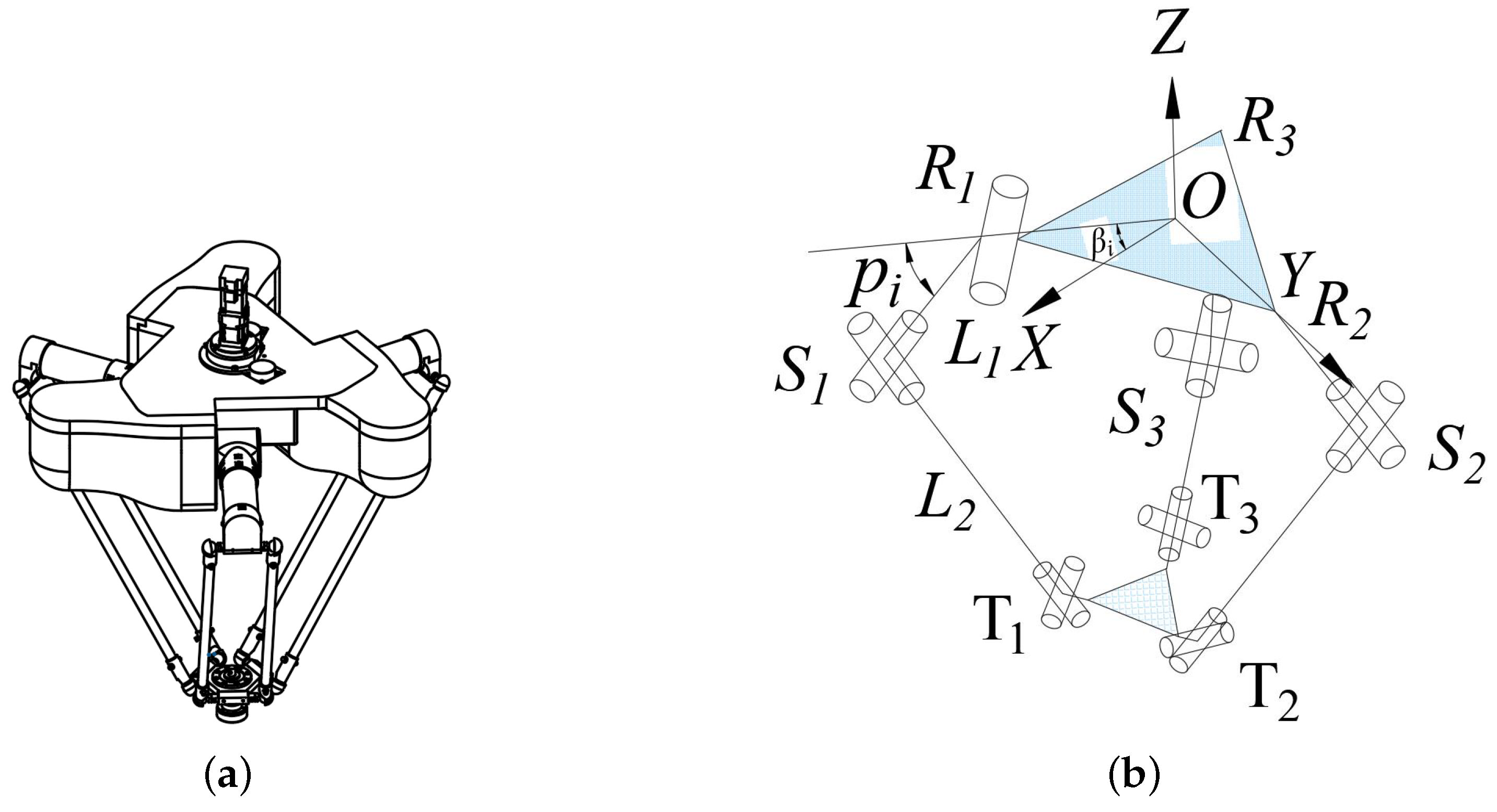
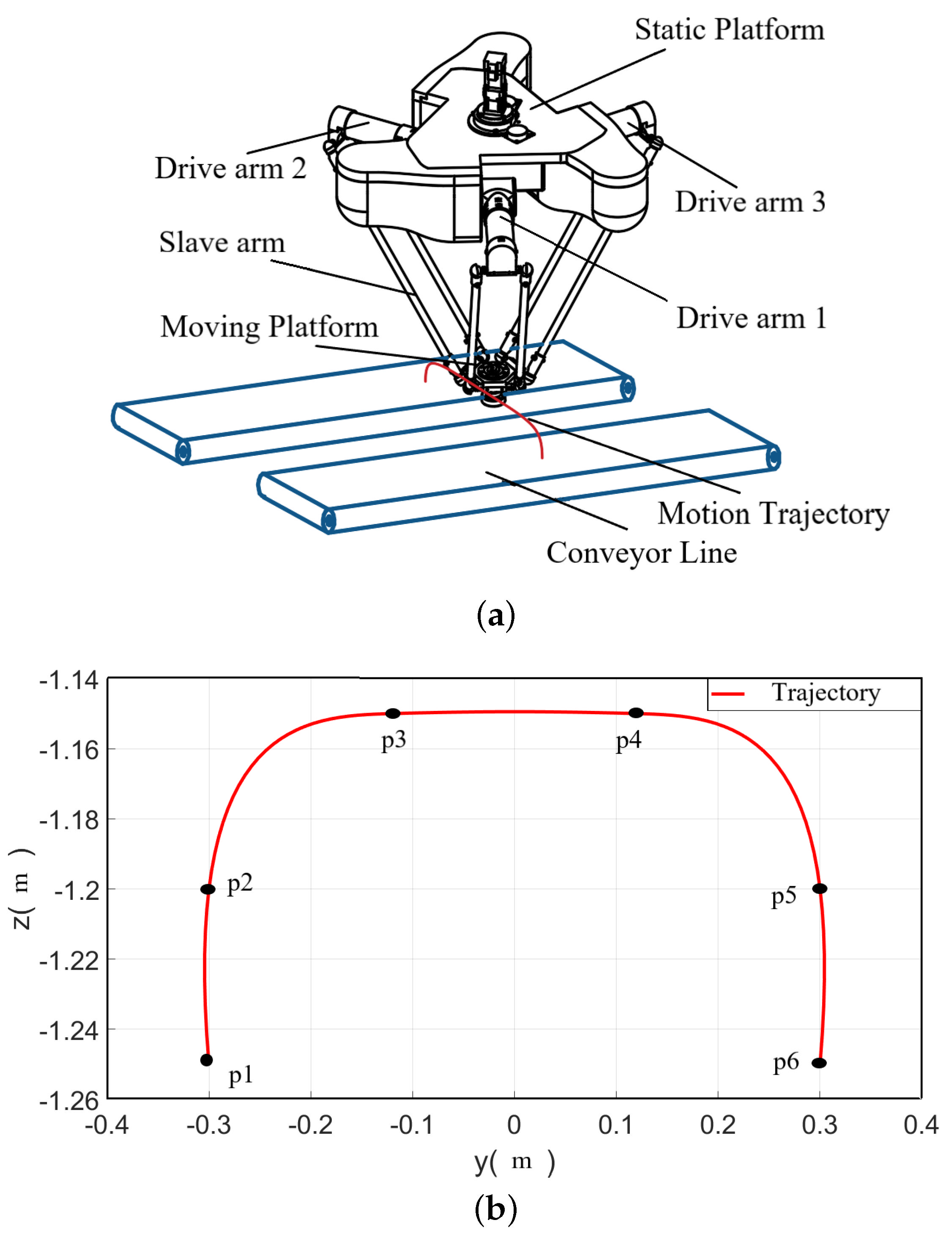
2. Delta Parallel Robot

Figure 1a shows the configuration of a three-degrees-of-freedom Delta robot. The Delta robot consists of a static platform, a moving platform, and three chains. The mobile platform is attached to the static platform by three symmetric chains, each of which includes a rotationally active proximal link and a spatial unactuated parallelogram composed of a spherical joint and link. The two ends of the telescopic rod in the middle are connected to the static platform and dynamic platform of the robot through u hinges. With this design, the movement can be delivered to the mobile platform through three chains.
The parallelogram of the parallel branch chain of the Delta parallel robot is simplified to a joint with two degrees of freedom along and perpendicular to the axis of the driving arm. According to the Delta parallel robot structure in Figure 1b. The coordinate system O X Y Z is established, with the center of the static platform as the coordinate origin. The inverse kinematic rotation angle of each drive arm can be obtained as shown in Equation (1):
p i = 2 arctan N i N i 2 + M i 2 P i 2 P i + M i
where
M i = 2 L 1 T x + r t cos β i r cos β i cos β i + T y + r t sin β i r sin β i sin β i N i = 2 L 1 T z P i = T x + r t cos β i r cos β i 2 + T y + r t sin β i r sin β i 2 + T z 2 + L 1 2 L 2 2
where p j is the angular displacement of the driver arm and β i represents the included angle between the robot static platform coordinate system and the driving arm. The radius of the static platform is recorded as r. The radius of the end moving platform is denoted r t . L 1 is the length of each drive arm. L 2 is the length of the parallel branch chain of the Delta parallel robot. T x , T y , and T z are the spatial coordinates of the center of the end moving platform of the parallel robot.

3. Optimal Time–Jerk Problem Description

A high-speed robot is expected to move quickly while performing pick-and-place tasks. However, increasing the frequency of pick and place unavoidably increases acceleration and jerk, thereby affecting the stability and position accuracy of the robot motion. Trajectory optimization is an effective scheme for reducing the robot jerk. An optimization process can be reviewed according to the following two aspects: firstly, finding the shortest movement time, and secondly, the motion stability during operation. Since the motion stability is mainly reflected in the acceleration, it is necessary to minimize the peak acceleration of the robot during the process.
Jerk is defined as the first derivative of acceleration with respect to time, which reflects the change rate of acceleration and is an important indicator for evaluating the smoothness of the robot motion. More specifically, the greater the jerkiness, the faster the acceleration change. According to Newton’s second law, acceleration affects the applied force on the robot driving joint. Accordingly, when the acceleration changes frequently, the motor that drives the joint should constantly change the output torque to control the robot movement, thereby leading to the chattering phenomenon in the motor and affecting the motion accuracy of the robot.
Therefore, it is essential to consider the variations in acceleration on the dynamic performance of the robot. This is especially the case for high-speed pick-and-place tasks. The larger the jerk, the lower the smoothness of the robot motion. In this paper, the average cumulative effect of trajectory mutation is defined as an index to evaluate the smoothness of the trajectory. To consider the total running time and the robot trajectory, the optimization objective can be mathematically expressed as follows:
κ 1 = i = 1 n 1 h i κ 2 = j = 1 N 1 t f 0 t f p j ( t ) 2 d t
where κ 1 and κ 2 are the objective functions for the motion time and the robot stability, respectively. Moreover, t f and p j denote the total movement time and the angular displacement of the driver arm, respectively. Equation (2) is subject to the following kinematic constraints:
p ˙ j v max p ¨ j a c c max p j j e r k max
where v max , a c c max , and j e r k max are the maximum values of the velocity, acceleration, and jerk, respectively.
The NURBS curve lies within the merging set of individual convex packages formed by the control vertices [29]. Consequently, this curve can be applied to convert the kinematic constraints to constraints on individual control vertices. The converted constraints can be expressed in the form below:
d j 1 v max d j 2 acc max d j 3 jerk max
However, the time and jerk are a set of conflicting objectives. On the on hand, as the running time reduces, the corresponding jerk fluctuations increase, which is not conducive to smoothing the trajectory. On the other hand, as the motion jerk reduces, the total motion time increases, which affects the efficiency of the operation. Accordingly, weighting factors are usually used in multi-objective optimization problems to optimize the running time and meet the acceleration requirements. According to the weight selection of the two optimization objectives, the optimization objective function is defined as follows:
f = i = 1 n w κ 1 κ 2 σ min σ max σ min
where w represents the weight factor and σ max and σ min are the boundary maximum and minimum of the objective function, respectively.

4. Trajectory Planning in Operation Space

4.1. Trajectory Description

Figure 2a shows the configuration of a high-speed parallel robot consisting of a static platform, three sets of driving arms, and a moving platform. A servo-motor and reducer are installed on the static platform. Moreover, each group of driving arms is composed of a driving arm and a slave arm, which are connected through spherical joints. The moving platform, which is connected to three groups of slave arms, can realize the translational movement of the robot along the x-, y-, and z-directions. Figure 2b shows the door-type trajectory, which is a typical trajectory in the operation space. During each grasping movement, the moving platform of the robot passes through the lift-off points p 1 p 3 in turn, and then passes through the set-down points p 4 p 6 . The height and span of the robot are 0.1 m and 0.6 m, respectively.

4.2. Trajectory Construction by Means of Fifth-Order NURBS Curve

The trajectory of an industrial robot is defined based on the sequential motion of a series of key points, which can be described using a polynomial function. In the present study, the NURBS curve is used to describe the trajectory of the end effector in the operation space. The NURBS curve can be obtained from the following expression:
p ( u ) = i = 0 n d i N i , k ( u )
where d i indicates the control vertex and N i , k is the basis function of the k-times NURBS. To describe the k-times NURBS curve, the domain node vector U should be defined in the form below:
U = u 0 , u 1 , , u k , u k + 1 , , u n , u n + 1 , , u n + k + 1
where n is the number of key points. Adopting the cumulative chord length method, the time vector t can be normalized to the knot vector u. This process can be mathematically expressed as follows:
u 0 = u 1 = = u k = 0 u n = u n + 1 = = u n + k + 1 = 1 u i = u i 1 + t i k t i k 1 j = 0 n 1 t j + 1 t j , i = k + 1 , , n 1
The k-times NURBS basis functions N i , k are obtained using the de Boor–Cox recurrence expression:
N i , 0 ( u ) = 1 u i < u < u i + 1 0 otherwise N i , k ( u ) = u u i u i + 1 u i N i , k 1 ( u ) + u i + k + 1 u u i + k + 1 u i + 1 N i + 1 , k 1 ( u ) make 0 0 = 0
The k-times NURBS curve equation of n + 1 interpolated key points p i is substituted into the nodes in [ u k , u n + k ] to obtain n + 1 equations that meet the interpolation conditions.
p u i + k = j = i i + k d j N j , k u i + k = p i , u i + k u k , u n + k i = 0 , 1 , , n
Then, the r-order derivative of p ( u i + k ) can be obtained as follows:
p r ( u ) = m = i k + r i d j r N j , k r ( u ) , u u i , u i + 1 m = i k , i k + 1 , , i
d j s = d j , s = 0 ( k + 1 s ) d j s 1 d j 1 s 1 u j + k ! s u j , s = 1 , 2 , , r
The control vertices are deducted, and the equation is shown as
A N d = p
where A N is the coefficient matrix and p is the motion parameter matrix.
For k-times NURBS curves, n + k boundary conditions require n + k control points. However, only n + 1 points satisfy equations; the other k 1 points satisfy the interpolation condition and can be obtained by tangent vector boundary conditions. Since the repetition of both end nodes is k + 1 , the first and last control vertices of the k-times B-sample curves can be used as data points of the constraint conditions. Accordingly, the boundary conditions can be obtained as follows:
p 0 = p u k = d 1 1 = k d 1 d 0 u k + 1 u 1 p n = p u n + k = d n + k 1 1 = k d n + k 1 d n + k 2 d n + 2 k 1 d n + k 1 p 0 = p u k = d 2 2 p n = p u n + k = d n + k + 2 2 p 0 = p u n = d 3 3 p n = p u n + k = d n + k 1 3

5. Improved Butterfly Optimization Algorithm

5.1. Butterfly Optimization Algorithm

In the butterfly optimization algorithm, each butterfly in the population is considered an independent search individual that releases a certain intensity of fragrance. Accordingly, the motion fitness changes when a single butterfly moves from one location to a new location during the searching process, and the fragrance spreads during the movement. Each butterfly perceives the fragrance of other butterflies, but the fragrance decays gradually with distance, and the butterfly moves to the location with the strongest fragrance. This is the main difference between the butterfly algorithm and other metaheuristics.
In the BOA, the value of the scent concentration f can be determined with respect to three parameters: the sensory modality ( c ) , the stimulus intensity ( I ) , and the power index ( a ) [30]. The perceptual morphology is the butterfly’s perception of the fragrance, which is an initialization constant of the algorithm and is usually used as an optimization parameter. The stimulus intensity ( I ) can be derived from the fitness function. Moreover, the parameter power index ( a ) is a constant, which varies in the range ( 0 , 1 ) . The basic form of the BOA can be expressed as follows:
f = c I a
The main stages of BOA can be summarized as follows:
( a ) Initialization stage, where the objective function is established according to the time–jerk requirements of the trajectory planning. Then, the trajectory is optimized by adjusting the control points of the NURBS. To this end, it is necessary to predefine the sensory modality, power index, switching probability, and initial population, and to calculate the corresponding fitness value.
( b ) Iteration stage, where the position of butterflies in the solution space is redistributed, and therefore the fitness value and fragrance of each butterfly should be recalculated. At this stage, it is necessary to conduct either a global or a local search. In the global search, the butterfly moves towards the butterfly g * with the largest fragrance value. This process can be mathematically expressed as follows:
x i t + 1 = x i t + ( r 2 × g * x i t ) × f i
where x i t + 1 and x i t are the solutions for the i-th butterfly in iteration t + 1 and t, and r is a random number within the range [0, 1]. In the present study, the global search of the JADE-GL tuned butterfly algorithm [29] is applied to perform a larger global search. Based on this algorithm, the potential solution can be expressed as follows:
x i t + 1 = x i t + ( r ( g i * x i t ) + ( 1 r ) ( x r 1 t x r 2 t ) ) × f i
where r 1 , r 2 are random numbers between 1 and the population size n, x i t denotes the solution corresponding to the i-th butterfly in the t-th iteration, g * denotes the optimal solution for the current iteration, f i denotes the fragrance emitted by the i-th butterfly, and r is a random number in the range ( 0 , 1 ) .
When a butterfly cannot sense the fragrance emitted by any other butterflies, it will take a random walk. At this time, corresponding to local search, the BOA can be expressed as
x i t + 1 = x i t + r 2 × x j t x k t × f i
where x i t and x k t denote the solutions corresponding to the j-th and k-th butterflies in the t-th iteration, respectively. Moreover, r is a random number in the range [ 0 , 1 ] . A switch probability p is used to switch between global and local searches in the BOA.
( c ) Termination stage, where the optimal solution is obtained. This condition is achieved when the obtained solution can satisfy the requirements, or the number of iterations reaches a certain value.

5.2. IBOA

Combining chaotic mapping and a fractional order with the standard butterfly optimization algorithm, an improved BOA (IBOA) is proposed to improve the solution accuracy and global optimization performance of the BOA.

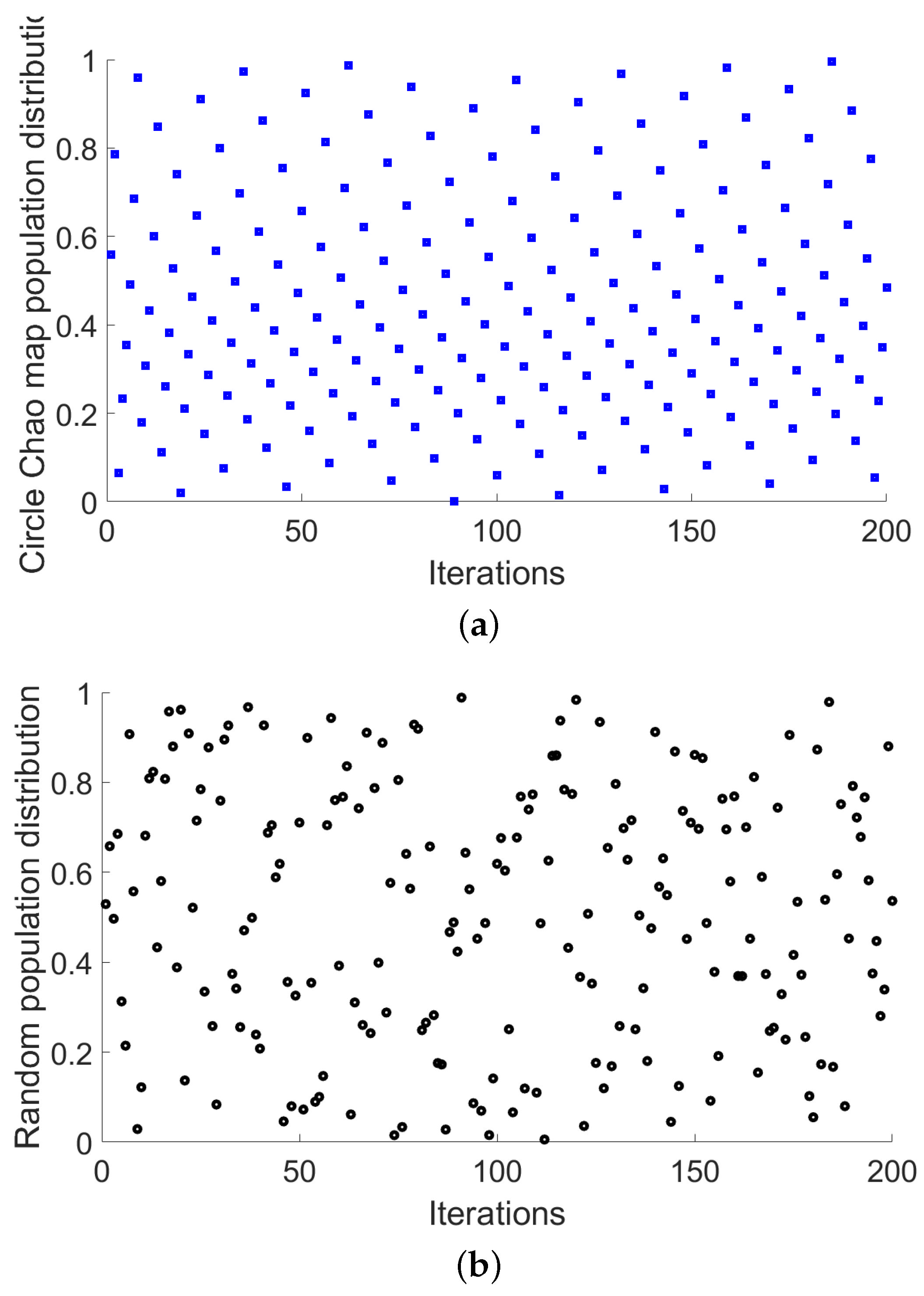
5.2.1. Chaotic Mapping

Chaotic mappings refer to multivariate nonlinear functions that can be used for nonlinear deterministic prediction of time series data to enhance the diversity of the initial population, thereby improving the global search capability of the BOA. In the present study, circle chaotic mapping [31] is used in the BOA algorithm to optimize the initial population.
The circle map can be expressed as follows:
x k + 1 = x k + b ( P 2 π ) sin 2 π x k mod ( 1 )
where b = 0.2 , and P = 0.5 is the control parameter. Equation (18) yields a chaotic mapping distribution in the range ( 0 , 1 ) .

5.2.2. Fractional Derivative

Aiming at preventing the BOA from falling into a local optimum, fractional derivatives are often used to improve the memory capacity and convergence of the BOA, enhance the memorability and search ability of iterative processes, and improve the accuracy of the solution. In this regard, Grunwald–Letnikov fractional differentiation is used in the present study to optimize BOA. The integral of integer order (G–L) is extended from integer order to fractional order using the gamma function. The α -order fractional differential can be expressed in the form below:
α D t α · η ( t ) = lim h 0 h α m = 0 ( ( t α ) / h ) ( 1 ) m Γ ( α + 1 ) Γ ( m + 1 ) Γ ( α m + 1 ) η ( t m h )
where D and α denote the fractional derivative and the order of the fractional derivative, respectively. When α > 0, G L denotes differentiation, while α > 0 refers to the integration. The fractional derivative combined with the BOA can be expressed as:
α D t α · x ( t ) = lim h 0 h α m = 0 ( t α ) / h ) ( 1 ) m Γ ( α + 1 ) Γ ( m + 1 ) Γ ( α m + 1 ) x ( t m h )
In order to combine with the discrete time-period in the trajectory planning, Equation (21) can be simplified to the form below:
D t v · x ( t ) = T v m = 0 c ( 1 ) m Γ ( v + 1 ) Γ ( m + 1 ) Γ ( v m + 1 ) x ( t m T )
where T and ζ are the sampling period and the truncation order, respectively. Based on Equation (18), the global search can be rewritten in the form below:
x i t + 1 x i t = r g i * x i t + ( 1 r ) x r 1 t x r 2 t × f i
Assuming v = T = 1 , Equation (22) can be re-expressed as
D t v · x i t + 1 = r g i * x i t + ( 1 r ) x r 1 t x r 2 t × f i
The first four terms of Equation (24) are
x i t + 1 = v x i t + 1 2 v ( 1 v ) x i t 1 1 6 v ( 1 v ) ( 2 v ) x i t 2 + 1 24 v ( 1 v ) ( 2 v ) ( 3 v ) x i t 3 + r g i * x i t + ( 1 r ) x r 1 t x r 2 t × f i
Moreover, a solution is randomly selected as an individual in the current solution. Then, a secondary local search is performed using this solution and its inverse solution. The quasi-Newton algorithm is used to implement a local search. The new position can be derived from the following expression:
x i d t + 1 = l b + ( u b l b ) × x k + 1
where l b and u b are the upper and lower limits of the NURBS curve control point adjustment, respectively, and x i d t + 1 is the solution for the i d -th butterfly in iteration t + 1 in the second search.
The main steps of the IBOA can be summarized as follows:
Step 1: Determine the number of butterflies n, the perceptual constant c, the stimulus factor I, and the switching probability parameter p. Initialize the population using circle chaos mapping;
Step 2: Solve the objective function.
Step 3: Derive the current optimal solution. To this end, use the global search in Equation (17) if rand < p , and use the local search in Equation (18) otherwise.
Step 4: Randomly select an individual from the current solution. A secondary local search is performed using this solution and its inverse solution. The quasi-Newton algorithm is used to implement a local search.
Step 5: Update the solution. The current optimal solution is obtained and compared with the best solution of the previous generation. Then, the optimal solution should be updated if the current optimal solution is better than the previous solution.
Step 6: Check the number of iterations. If the number of iterations reaches a certain value, the calculation ends. Check whether the termination condition is satisfied. If it is not satisfied, return to step 3.
Figure 3 shows the flowchart of the improved butterfly optimization algorithm.

6. Simulation Test and Results Analysis

6.1. Experimental Test of IBOA

6.1.1. Test of IBOA Population

In order to evaluate the performance of the IBOA, experiments were carried out, and the results are analyzed in this section. The population distribution and the convergence speed of the IBOA are analyzed.
Figure 4 reveals, with the help of the circle chaotic map, that the population distribution of the butterfly optimization algorithm is more uniform than a random distribution.

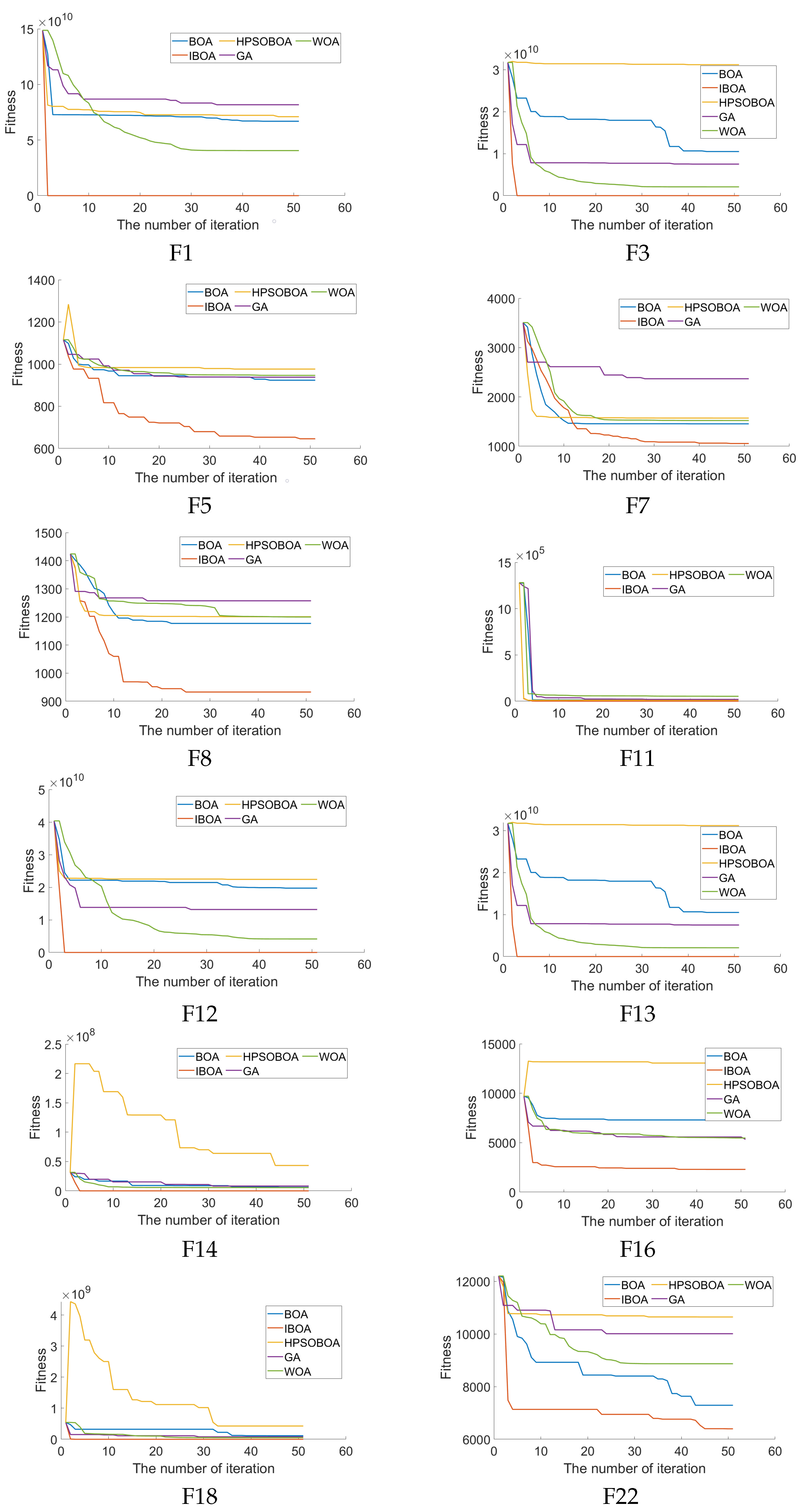
6.1.2. Results for Benchmark Test Functions

In order to show the effectiveness of the IBOA, the commonly used test functions of CEC217 were used in the experiments. The results are compared with those obtained from WOA, GA, BOA, and HPSOBOA optimization algorithms.
For each test function shown in Table 1, Table 2 and Table 3, each optimization algorithm was run 30 times, starting from randomly generated populations. Figure 5 shows the competitiveness of different algorithms for three test functions.
The comparison of the convergence curves of different algorithms reveals that the IBOA is very competitive compared with other metaheuristic techniques for solving optimization problems.

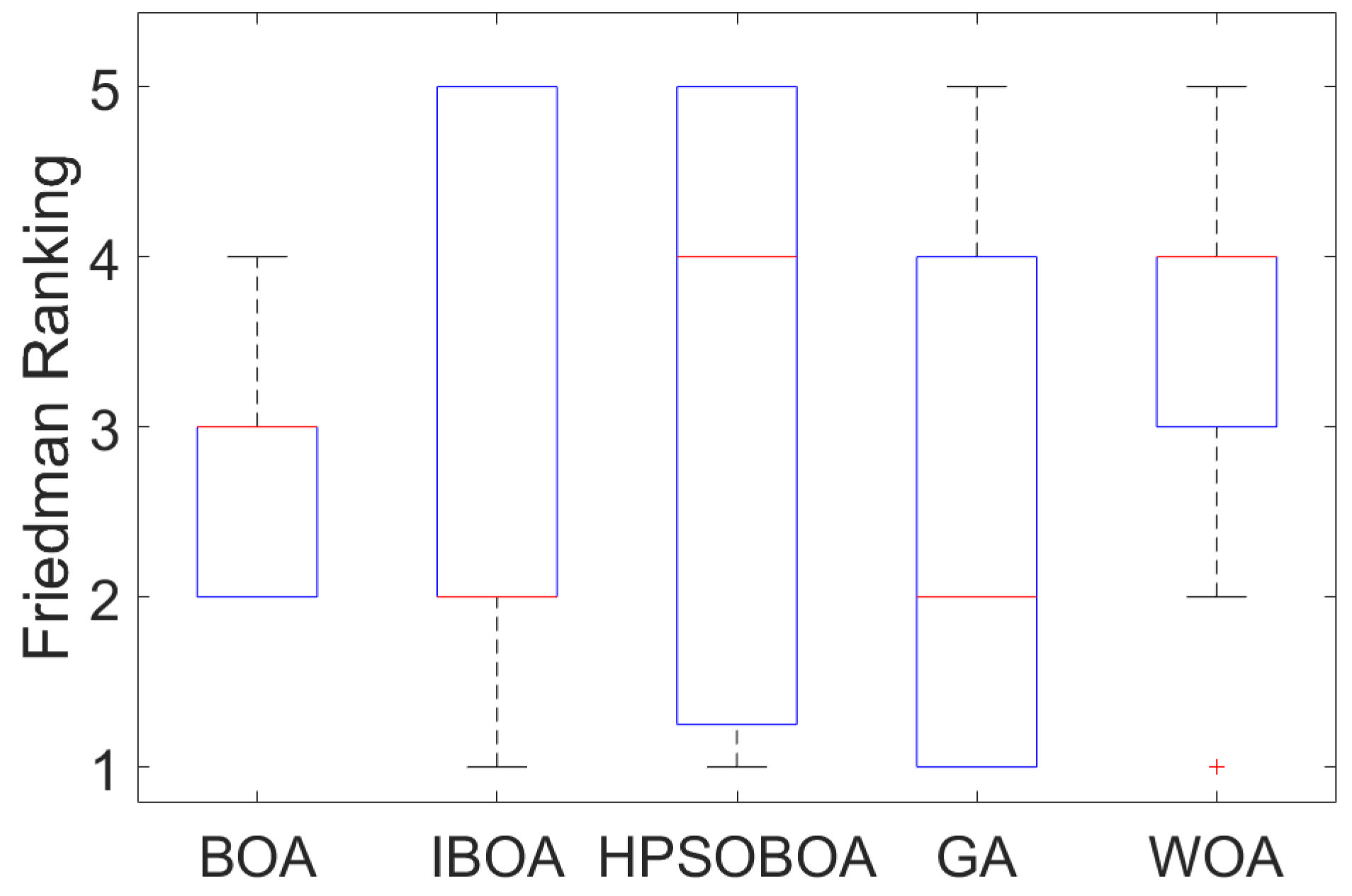
6.1.3. Non-Parametric Test

In order to better test the performance of the algorithm, a series of test methods were used to evaluate the advantages and disadvantages of the algorithm. Among them, the statistical method is considered to be an effective method, including a parametric test and a non-parametric test. For the comparison of various algorithms, the hypothesis estimation method is not considered to be conducive to the evaluation of the advantages and disadvantages of the algorithm. The newly developed algorithm’s statistical performance was verified by employing a non-parametric statistical test.
In this non-parametric test, each algorithm is executed for 30 independent runs, with 20 populations, for 50 iterations. A non-parametric Wilcoxon test was used to evaluate the differences between paired samples.The p-values achieved in the test are shown in Table 4, indicating that the IBOA algorithm is mathematically significantly superior.
Unlike the Wilcoxon rank test, the Friedman test is used to obtain a ranking for multiple algorithms. For the above test functions, IBOA’s performance was better than the other algorithms. This non-parametric test is used to rank the algorithms. According to the box diagram shown in Figure 6, the test results show that the mean rank for IBOA is the minimum among all the algorithms.

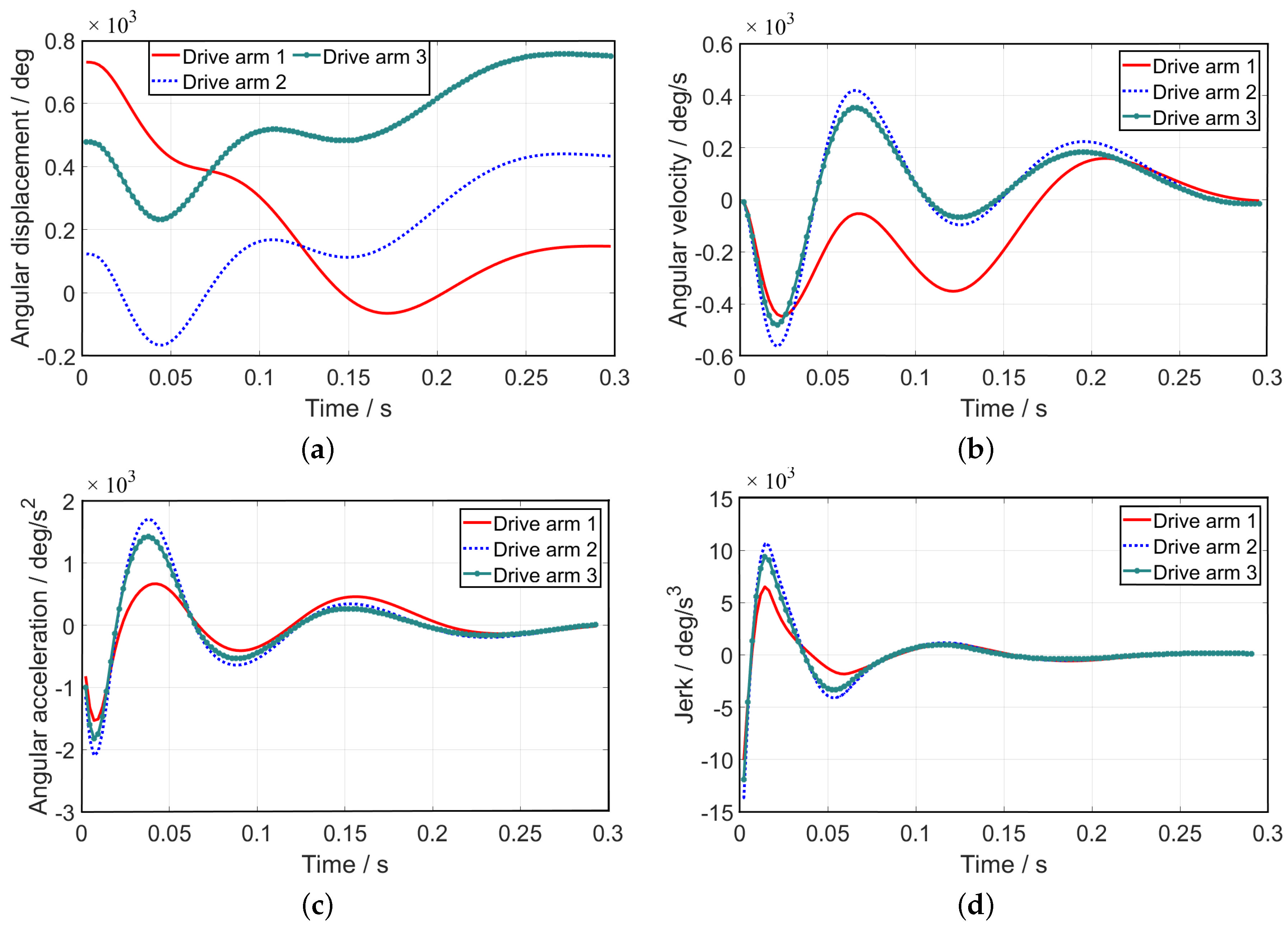
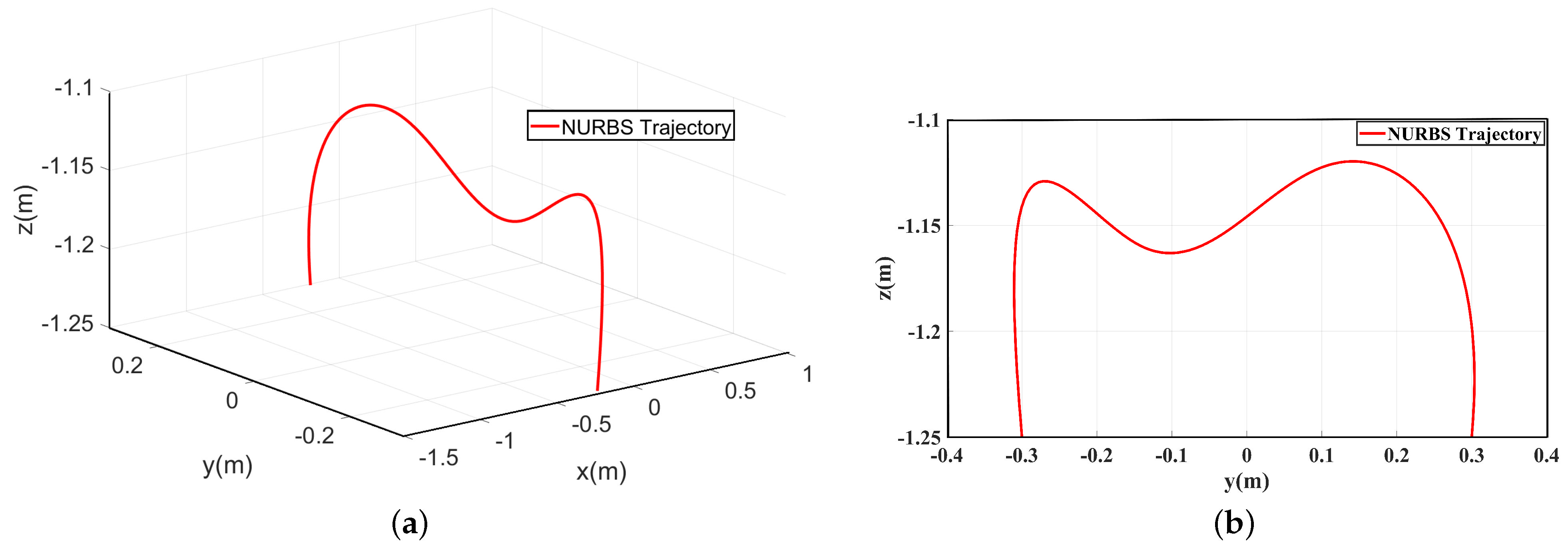
6.2. Trajectory Planning for Delta High-Speed Parallel Robots

It should be indicated that all calculations were carried out in the MATLAB environment. Six key points of the door-type trajectory were preset, and then optimal time–jerk trajectory planning was performed in the Cartesian space, considering kinematic constraints. The values of the trajectory key points are listed in Table 5, and the kinematic constraints of the robot are shown in Table 6.
In all calculations, the quintic NURBS curve interpolation was used to obtain the trajectory in Cartesian space. The corresponding displacement, velocity, acceleration, and jerk curves of the three drive arms in the joint space derived from the kinematic inverse solution are depicted in Figure 7.

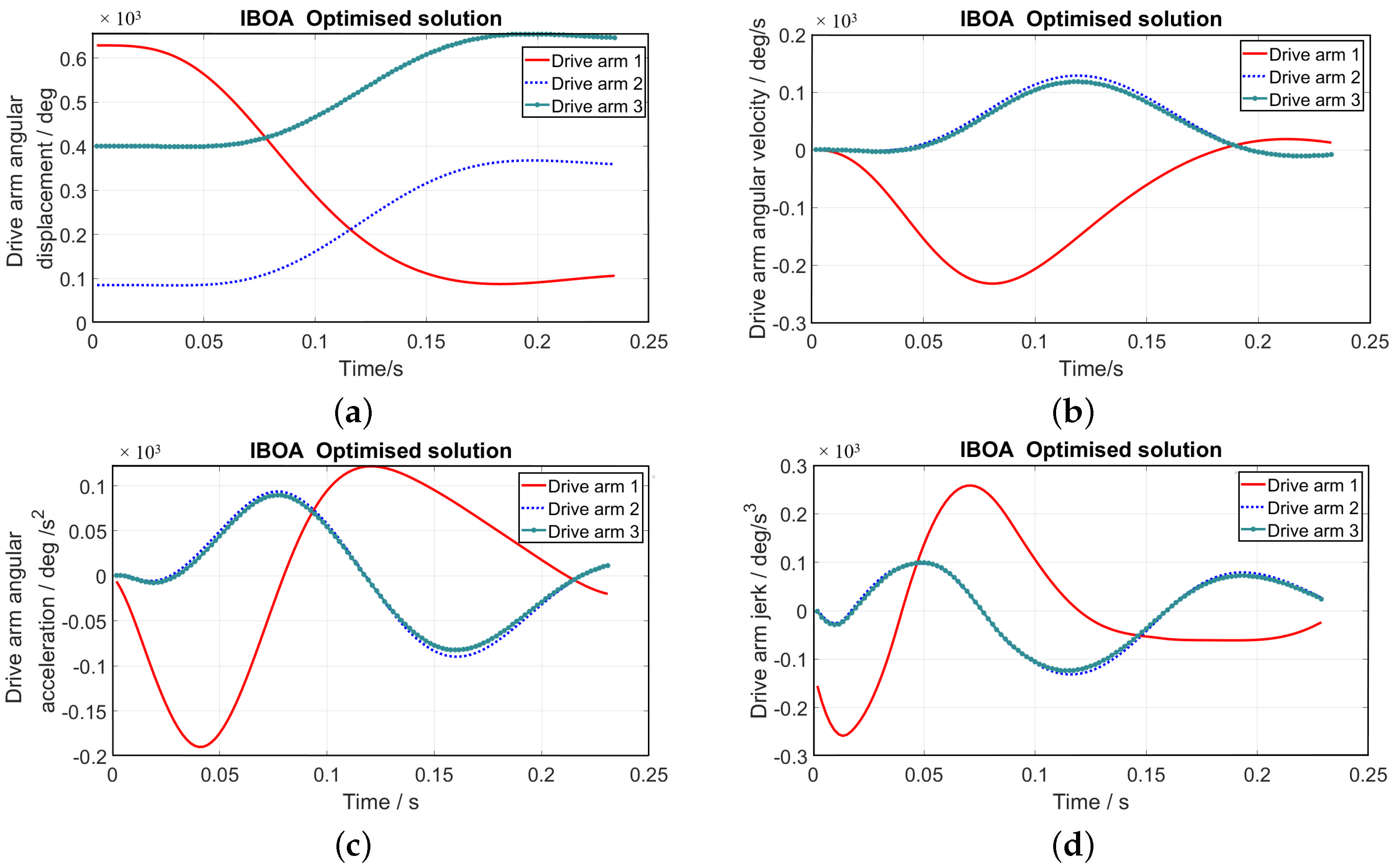
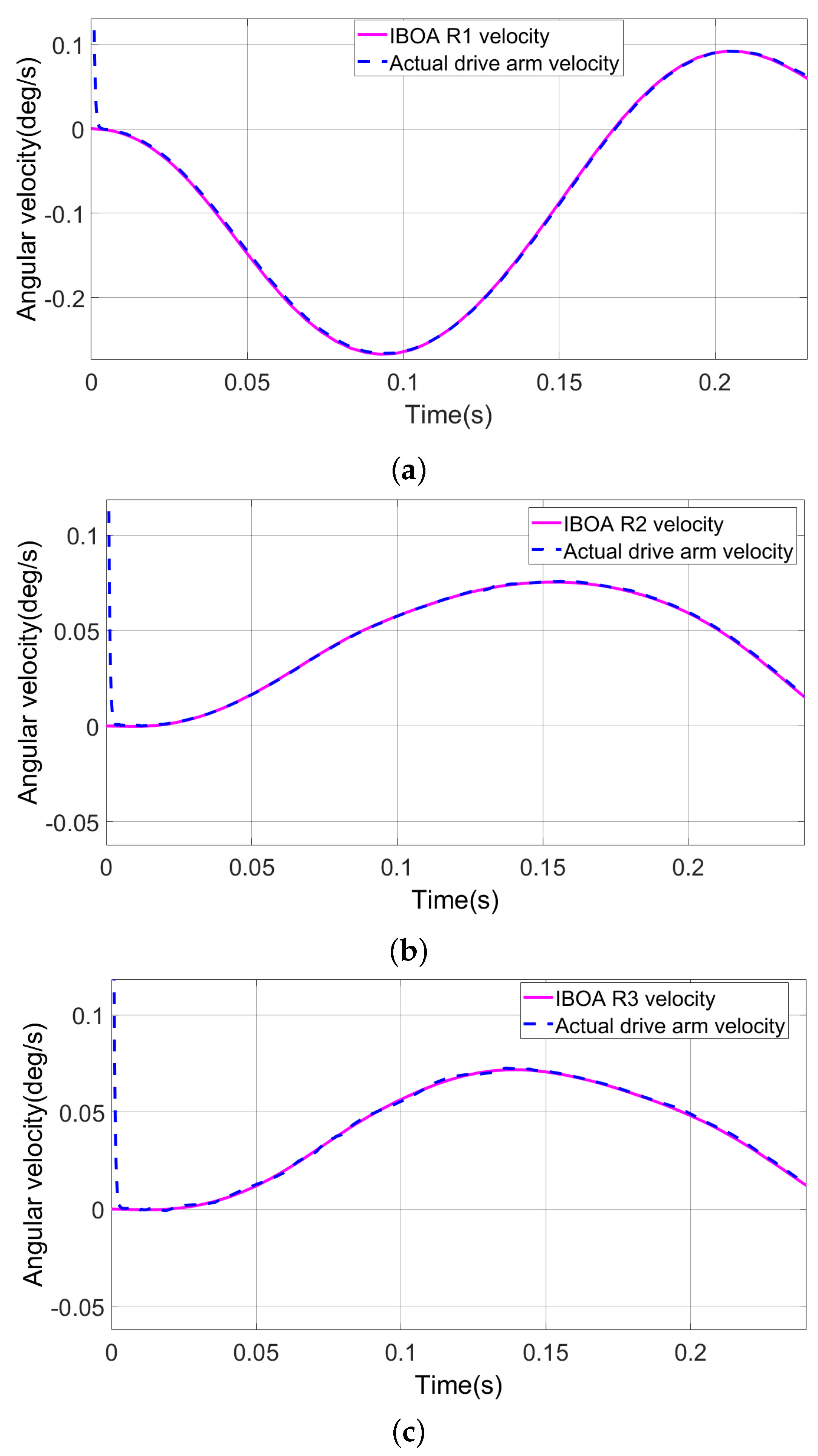
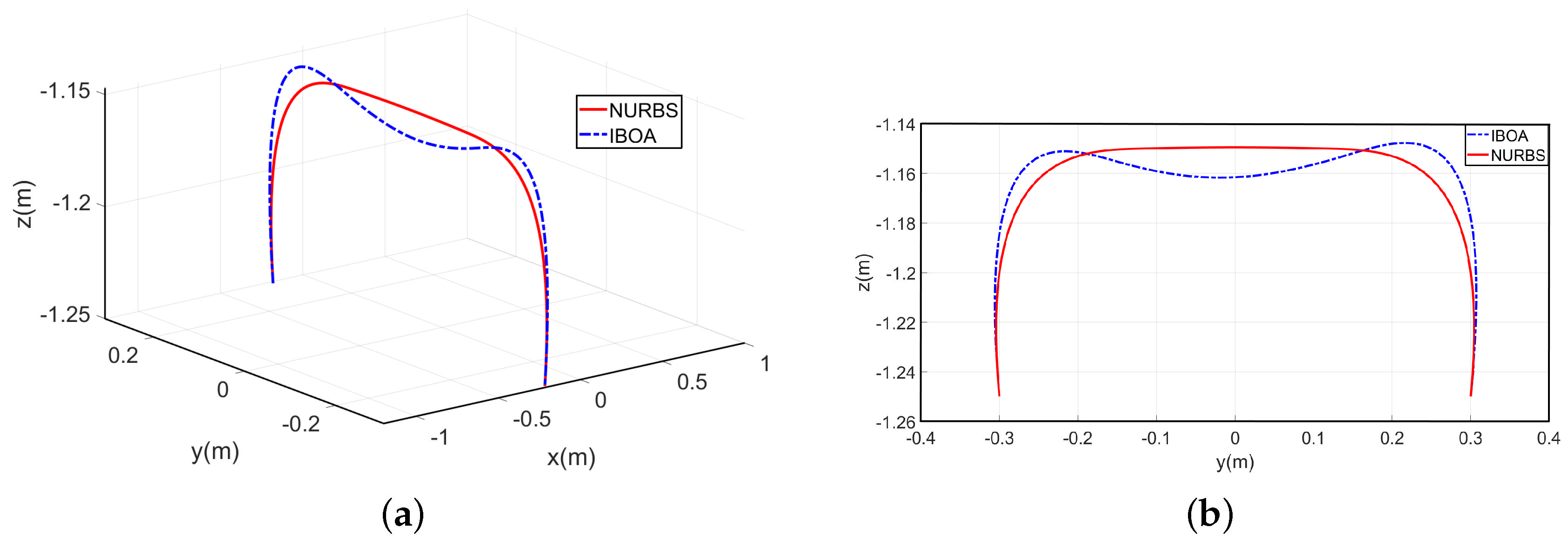
6.3. Verification of the IBOA Trajectory Optimization

Taking the evaluation indices of two optimization objectives as the test standard, the obtained results from IBOA, WOA, GA, HPSOBOS, and BOA were compared. In all simulations, the population size and the maximum number of iterations were set to 50. The weight factors of the selected time and impact were set to 0 and 1, respectively. The simulation results are shown in Figure 8.
Figure 8 reveals that WOA converges to 0.06 after 26 iterations, but the convergence is premature. Moreover, GA and HPSOBOA converge at the 6th generation, while the original BOA converges at the 12th generation, but they simply fall into the local convergence, so that their optimization results do not meet the requirements. The lowest optimization results were achieved from the IBOA, indicating the high optimization accuracy of this algorithm. More specifically, the IBOA reaches an optimized value of 0.03 after 32 steps, indicating that IBOA can achieve reasonable optimization results.
Table 7 shows the optimization results of different algorithms for the motion time. It was found that the IBOA reduces the motion time by 16.2 % , while WOA, GA, HPSOBOA, and BOA reduce the robot motion time by 14.1 % , 15.5%, 12.7 % , and 12.7 % , respectively. The optimization results for the second optimization objective are shown in Table 8. It can be observed that the best optimization effect on the jerk was 87.6 % , which was achieved using the IBOA. The obtained results demonstrate that the IBOA algorithm outperformed the other algorithms in terms of the time–jerk trajectory planning of the robot.
The motion parameters of the drive arm optimized by IBOA are shown in Figure 9. It can be observed that the optimized motion time for IBOA decreases from 0.28 s to 0.2346 s. Moreover, the maximum jerk values of the driving arm before and after optimization were 2.5 × 10 3 deg / s 3 and 0.3089 × 10 3 deg / s 3 , respectively.
It is found that the displacement curve changes after optimization. Due to the change in the position of the control point, the trajectories before and after optimization are different, and therefore the displacement curve changes.
The optimized trajectory profile in Figure 10 indicates that after IBOA optimization, the trajectory produces deformation along the Z-axis direction. This may be attributed to the deviations of the regenerated curve from the control point after changing the key point position for the high-order NURBS curve, which deform the generated trajectory. It is worth noting that this phenomenon is not conducive to robot motion.
The boundary constraint of the control point is added to the optimization process, and the adjustment range of the key point is between 0.05. The optimized trajectory is shown in Figure 11. Comparing the running trajectory before and after the optimization in the operation space reveals that the optimization result after setting the boundary conditions effectively reduces the deformation. In the optimized trajectory, the jerk value reduces by 76.3 % , which shows the effectiveness of the optimization method.

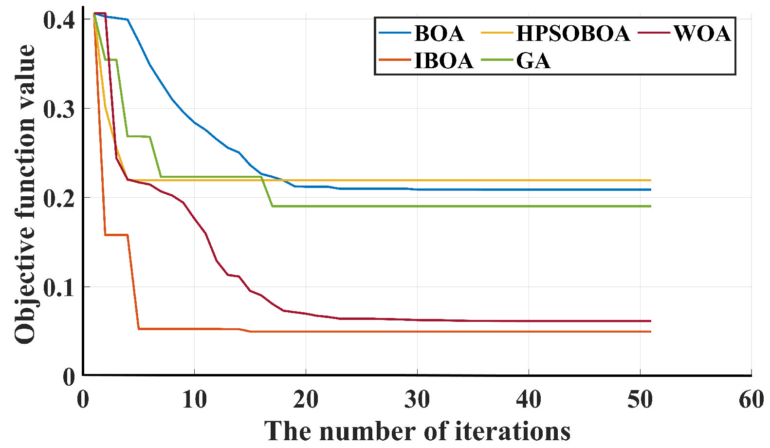
6.4. Simulation Experiments for Trajectory Optimization

In this section, the planning optimization methods designed above are verified via experiments. Figure 12 shows the Delta parallel robot prototype, including the frame, the robot, and its control system. This part is based on the robot as an example, and the driving parameters optimized by the IBOA algorithm are used to control the robot pickup motion.
The driving speed parameters optimized by the IBOA algorithm and the non-optimized driving speed parameters were used as inputs, respectively, to carry out the picking motion test of the robot and to monitor the actual motor speed. The actual motor speed for the IBOA is shown in Figure 13.
The vibration accelerations of the mobile platform at the end of the robot corresponding to two groups of different speed parameters are shown in Figure 14 and Figure 15, respectively. The simulation results show that the driving parameters optimized by the IBOA can effectively reduce the vibration acceleration of the Delta parallel robot in high-speed motion. The results show that the optimization method is effective.

7. Conclusions

In this paper, an improved butterfly optimization algorithm was proposed to solve the trajectory optimization problem for the Delta high-speed parallel robot. By optimizing the trajectory, the picking efficiency was improved and the residual vibration of the robot was reduced. The main contributions are as follows.
  • The trajectory planning was carried out in Cartesian space, and the NURBS curve was used to generate the trajectory. The picking trajectory was designed according to the actual robot picking span, and the displacement, velocity, acceleration, and jerk curve of each driving arm were obtained through velocity, acceleration, and jerk constraints.
  • In order to improve the dynamic performance of the robot, BOA was used for optimization. Aiming at resolving the problems of the standard BOA, such as low convergence speed and ease of falling into a local optimum in multi-objective optimizations, chaotic mapping and fractional differentiation were used to improve the butterfly optimization algorithm. This not only expanded the search scope of the algorithm but also increased the iteration memory, which helped to improve the convergence speed and accuracy. Then, numerous simulation tests were carried out. The obtained results showed that the improved algorithm had more significant competitiveness and could reduce the jerk in multi-objective optimizations by 87.6%.
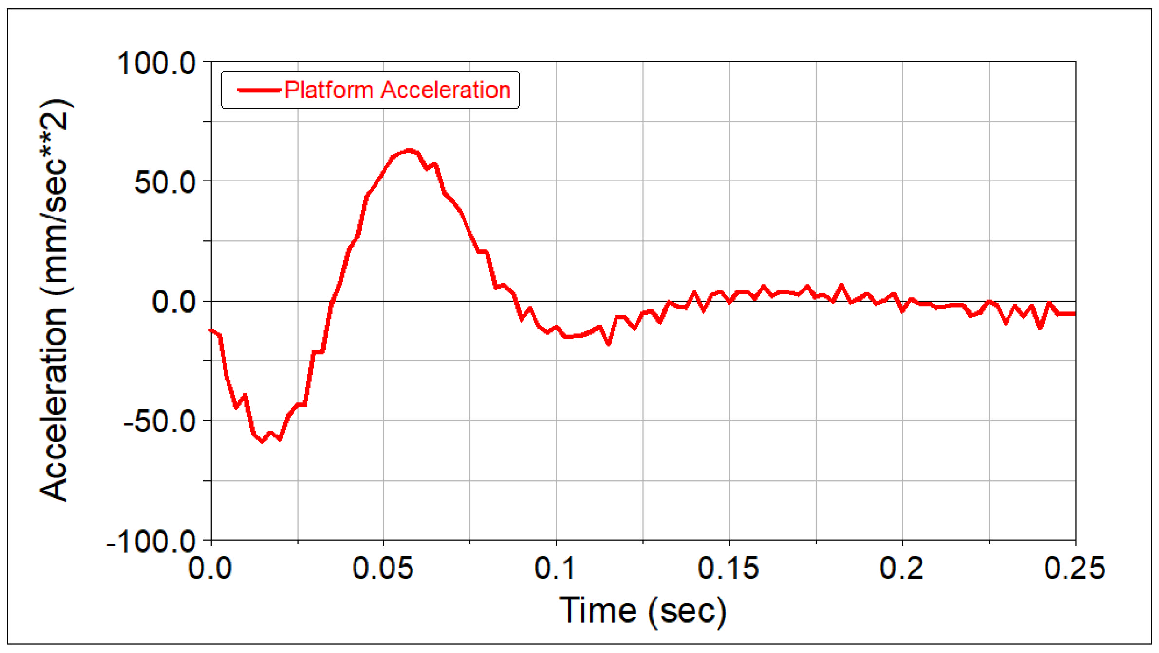
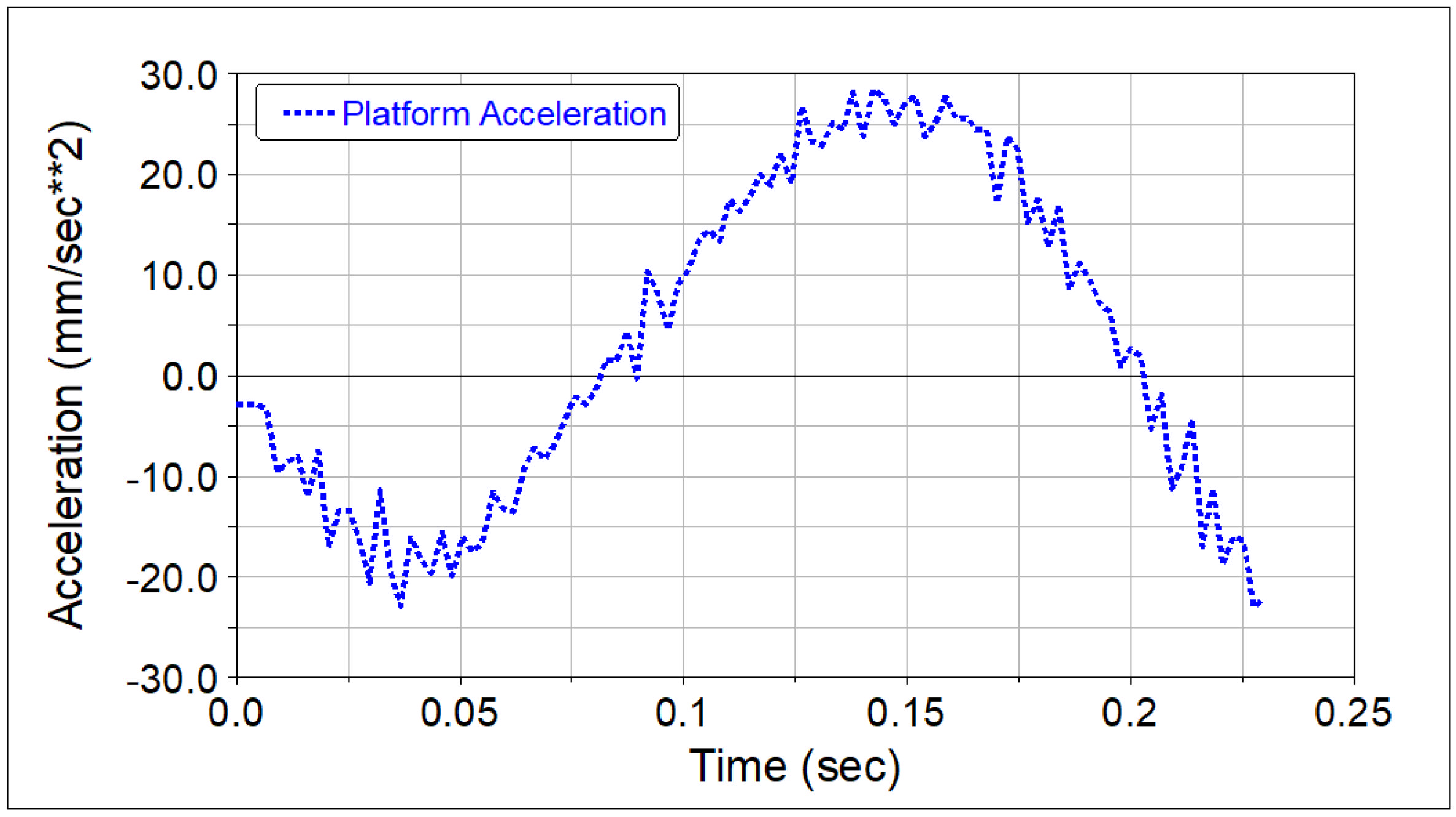
  • The vibration accelerations of the robot terminal platform before and after optimization were compared numerically. The simulation results showed that the optimized trajectory effectively reduced the vibration acceleration of the terminal platform.
The proposed trajectory optimization method can also be applied to other parallel robots to improve their dynamic characteristics. This paper has mainly focused on the analysis of the kinematics of the robot and on improving the dynamic performance based on the dynamic analysis. However, the motion span of the end platform may affect the performance of the robot. To ensure efficient and effective improvement of the dynamic performance of the robot, the dexterous workspace within 600 mm of the robot can be analyzed.

Author Contributions

P.W. wrote the manuscript and performed the experiments; Z.W. analyzed the data and revised the manuscript; H.J. assisted in completing the simulation test; P.Z. mainly assisted in the translation and proofreading of the manuscript. All authors discussed the results and commented on the manuscript. All authors have read and agreed to the published version of the manuscript.

Funding

This work was supported in part by the Key R&D Projects for International Cooperation in Shanxi Province under Grant 201903D421015 and in part by the Scientific and Technological Innovation Programs of Higher Education Institutions in Shanxi Province under Program 2019L0936.

Institutional Review Board Statement

Not applicable.

Informed Consent Statement

Not applicable.

Data Availability Statement

Not applicable.

Conflicts of Interest

The authors declare no conflict of interest.

References

  1. Patel, Y.D.; George, P.M. Parallel manipulators applications—A survey. Mod. Mech. Eng. 2012, 2, 57–64. [Google Scholar] [CrossRef]
  2. Song, X.G.; Zhao, Y.J.; Jin, L.; Zhang, P.; Chen, C.W. Dynamic feedforward control in decoupling space for a four-degree-of-freedom parallel robot. Int. J. Adv. Robot. Syst. 2019, 2, 1–10. [Google Scholar]
  3. Connolly, C. ABB high-speed picking robots establish themselves in food packaging. Ind. Robot. Int. J. 2007, 34, 281–284. [Google Scholar] [CrossRef]
  4. Company, O.; Marquet, F.; Pierrot, F. A new high-speed 4-DOF parallel robot synthesis and modeling issues. IEEE Trans. Robot. Autom. 2003, 19, 411–420. [Google Scholar] [CrossRef]
  5. Chen, Y.D.; Li, L. Predictable trajectory planning of industrial robots with constraints. Appl. Sci. 2018, 8, 2648. [Google Scholar] [CrossRef]
  6. Stilman, M. Global manipulation planning in robot joint space with task constraints. IEEE Trans. Robot. 2010, 26, 576–584. [Google Scholar] [CrossRef]
  7. Mei, J.P.; Zang, J.W.; Qiao, Z.Y.; Liu, S.T.; Song, T. Trajectory planning of 3-DOF Delta parallel manipulator. J. Mech. Eng. 2016, 52, 9–17. [Google Scholar] [CrossRef]
  8. Li, Y.H.; Huang, T.; Chetwynd, D.G. An approach for smooth trajectory planning of high-speed pick-and-place parallel robots using quintic B-splines. Mech. Mach. Theory 2018, 126, 479–490. [Google Scholar] [CrossRef]
  9. Gauthier, J.F.; Angeles; Nokleby, S. Optimization of a test trajectory for SCARA systems. In Advances in Robot Kinematics: Analysis and Design; Springer: Dordrecht, The Netherlands, 2008; pp. 225–234. [Google Scholar]
  10. Su, T.T.; Cheng, L.; Wang, Y.K.; Liang, X.; Zheng, J.; Zhang, H.J. Time-optimal trajectory planning for delta robot based on quintic pythagorean-hodograph curves. IEEE Access 2018, 6, 28530–28539. [Google Scholar] [CrossRef]
  11. Wang, S.A.; Wu, S.; Kang, C.; Li, X. Trajectory planning of a parallel manipulator based on kinematic transmission property. Intell. Serv. Robot. 2015, 8, 129–139. [Google Scholar] [CrossRef]
  12. Han, S.J.; Shan, X.C.; Fu, J.X.; Xu, W.J.; Mi, H.Y. Industrial robot trajectory planning based on improved pso algorithm. J. Phys. Conf. Ser. 2021, 1820, 012185. [Google Scholar] [CrossRef]
  13. Perez-Carabaza, S.; Besada-Portas, E.; Lopez-Orozco, J.A.; Jesus, M. Ant colony optimization for multi-UAV minimum time search in uncertain domains. Appl. Soft Comput. 2018, 62, 789–806. [Google Scholar] [CrossRef]
  14. Zhang, X.Q.; Ming, Z.F. Trajectory planning and optimization for a Par4 parallel robot based on energy consumption. Appl. Sci. 2019, 9, 2770. [Google Scholar] [CrossRef]
  15. Zhang, Q.; Li, S.; Guo, J.X.; Gao, X.S. Time-optimal path tracking for robots under dynamics constraints based on convex optimization. Robotica 2016, 34, 2116–2139. [Google Scholar] [CrossRef]
  16. Yu, X.L.; Dong, M.S.; Yin, W.M. Time-optimal trajectory planning of manipulator with simultaneously searching the optimal path. Comput. Commun. 2022, 181, 446–453. [Google Scholar] [CrossRef]
  17. Yu, R.; Wang, C.J.; Guo, Y.C.; Zhang, Y.P. Time-optimal trajectory planning of robot based on breed algorithm. Mech. Drive 2018, 42, 55–59. [Google Scholar]
  18. Chen, Y.; Yan, L.; Wei, H.; Wang, T. Optimal trajectory planning for industrial robots using harmony search algorithm. Ind. Robot. Int. J. 2013, 40, 502–512. [Google Scholar] [CrossRef]
  19. Wang, W.J.; Tao, Q.; Cao, Y.T.; Wang, X.H.; Zhang, X. Robot time-optimal trajectory planning based on improved cuckoo search algorithm. IEEE Access 2020, 8, 86923–86933. [Google Scholar] [CrossRef]
  20. Liu, C.; Cao, G.H.; Qu, Y.Y.; Cheng, Y.M. An improved PSO algorithm for time-optimal trajectory planning of Delta robot in intelligent packaging. Int. J. Adv. Manuf. Technol. 2020, 107, 1091–1099. [Google Scholar] [CrossRef]
  21. Zhou, J.; Cao, H.J.; Jiang, P.; Li, C.B.; Yi, H.; Liu, M.L. Energy-Saving Trajectory Planning for Robotic High-Speed Milling of Sculptured Surfaces. IEEE Trans. Autom. Sci. Eng. 2021, 19, 2278–2294. [Google Scholar] [CrossRef]
  22. Wang, Z.Q.; Peng, J.Z.; Ding, S. A Bio-inspired trajectory planning method for robotic manipulators based on improved bacteria foraging optimization algorithm and tau theory. Math. Biosci. Eng. 2022, 19, 643–662. [Google Scholar] [CrossRef] [PubMed]
  23. Lu, S.; Zhao, J.D.; Jiang, L.; Liu, H. Time-jerk optimal trajectory planning of a 7-DOF redundant robot. Turk. J. Electr. Eng. Comput. Sci. 2017, 25, 4211–4222. [Google Scholar] [CrossRef]
  24. Wang, T.; Xin, Z.J.; Miao, H.B.; Zhang, H.; Chen, Z.Y.; Du, Y.F. Optimal trajectory planning of grinding robot based on improved whale optimization algorithm. Math. Probl. Eng. 2020, 2020, 3424313. [Google Scholar] [CrossRef]
  25. Bureerat, S.; Pholdee, N.; Radpukdee, T.; Jaroenapibal, P. Self-adaptive MRPBIL-DE for 6D robot multiobjective trajectory planning. Expert Syst. Appl. 2009, 136, 133–144. [Google Scholar] [CrossRef]
  26. Huang, J.; Hu, P.; Wu, K.; Zeng, M. Optimal time-jerk trajectory planning for industrial robots. Mech. Mach. Theory 2018, 121, 530–544. [Google Scholar] [CrossRef]
  27. Chen, D.; Li, S.; Wang, J.F.; Feng, Y.; Liu, Y. A multi-objective trajectory planning method based on the improved immune clonal selection algorithm. Robot. Comput. Integr. Manuf. 2019, 59, 431–442. [Google Scholar] [CrossRef]
  28. Yin, S.; Ji, W.; Wang, L. A machine learning based energy efficient trajectory planning approach for industrial robots. Procedia CIRP 2019, 81, 429–434. [Google Scholar] [CrossRef]
  29. Rauf, H.T.; Bangyal, W.; Lali, M.I. An adaptive hybrid differential evolution algorithm for continuous optimization and classification problems. Neural Comput. Appl. 2021, 33, 10841–10867. [Google Scholar] [CrossRef]
  30. Arora, S.; Singh, S. Butterfly optimization algorithm: A novel approach for global optimization. Soft Comput. 2018, 23, 715–734. [Google Scholar] [CrossRef]
  31. Arora, S.; Singh, S. An improved butterfly optimization algorithm with chaos. J. Intell. Fuzzy Syst. 2017, 32, 1079–1088. [Google Scholar] [CrossRef]
Figure 1. Delta parallel robot. (a) Prototype of Delta parallel robot; (b) Sketch of Delta parallel robot.
Applsci 12 08145 g001
Figure 2. Configuration of the Delta parallel robot and motion trajectory in the operating space. (a) Schematic configuration of the parallel robot and its motion trajectory. (b) NURBS curve in the operating space.
Applsci 12 08145 g002
Figure 3. Flowchart of the improved butterfly optimization algorithm for time–impact optimized trajectory planning.
Applsci 12 08145 g003
Figure 4. Population distribution comparison map. (a) Cirlce mapping population distribution; (b) Random population distribution.
Applsci 12 08145 g004
Figure 5. Comparison of convergence curves of IBOA and other algorithms obtained in some of the benchmark problems.
Applsci 12 08145 g005
Figure 6. Box-plot comparison of results of IBOA with the basic methods using CEC17 functions.
Applsci 12 08145 g006
Figure 7. NURBS curve motion parameters. (a) The drive arm angular displacement; (b) The drive arm angular velocity; (c) The drive arm angular acceleration; (d) The drive arm angular jerk.
Applsci 12 08145 g007
Figure 8. Distribution of convergence rates for different algorithms.
Applsci 12 08145 g008
Figure 9. IBOA-optimized motion parameters. (a) The drive arm angular displacement with the trajectory planning based on IBOA. (b) The drive arm angular velocity with the trajectory planning based on IBOA. (c) The drive arm angular acceleration with the trajectory planning based on IBOA. (d) The drive arm angular jerk with the trajectory planning based on IBOA.
Applsci 12 08145 g009
Figure 10. Optimized trajectory curve using IBOA. (a) The trajectory curve in operating space; (b) YOZ view of trajectory curve.
Applsci 12 08145 g010
Figure 11. The motion trajectory with optimization using IBOA. (a) The trajectory curve in operating space after optimization. (b) YOZ view of trajectory curve after optimization.
Applsci 12 08145 g011
Figure 12. Delta robot.
Applsci 12 08145 g012
Figure 13. Actual angular velocity of each drive arm. (a) Actual angular velocity of R1 drive arm; (b) Actual angular velocity of R2 drive arm; (c) Actual angular velocity of R3 drive arm.
Applsci 12 08145 g013
Figure 14. Non-optimized vibration acceleration of robot platform.
Applsci 12 08145 g014
Figure 15. Vibration acceleration of robot platform after IBOA optimization.
Applsci 12 08145 g015
Table 1. Unimodal benchmark test functions.
Formula of FunctionDimRange f min
F 1 ( x ) = i = 1 N x i 2 30 [ 100 , 100 ] 0
F 2 ( x ) = i = 1 N x i + i = 1 N x i 30 [ 10 , 10 ] 0
F 3 ( x ) = i = 1 N j 1 i x i 2 30 [ 100 , 100 ] 0
F 4 ( x ) = max i x i , 1 i N 30 [ 100 , 100 ] 0
F 5 ( x ) = i = 1 N 1 100 x i + 1 x i 2 2 + x i 1 2 30 [ 30 , 30 ] 0
F 6 ( x ) = i = 1 N 1 x i + 0.5 2 30 [ 100 , 100 ] 0
F 7 ( x ) = i = 1 N 1 i x i 4 + random [ 0 , 1 ] 30 [ 1.28 , 1.28 ] 0
Table 2. Multimodal benchmark test functions.
Formula of FunctionDimRange f min
F 8 ( x ) = i = 1 N x i sin x i 30 [ 500 , 500 ] −2094.9
F 9 ( x ) = i = 1 N x i 2 10 cos 2 π x i + 10 30 [ 5.12 , 5.12 ] 0
F 10 ( x ) = 20 exp 0.2 1 N i = 1 N x i 2 exp 1 N i = 1 N cos 2 π x i + 20 + e 30 [ 32 , 32 ] 0
F 11 ( x ) = 1 4000 i = 1 N x i 2 i = 1 N cos x i i + 1 30 [ 600 , 600 ] 0
F 12 ( x ) = π N 10 sin π y 1 + i = 1 N 1 y i 1 2 1 + 10 sin π y i + 1 + y n + 1 2 y i N 1 = 1 + x i + 1 4 u x i , 10 , 100 , 4 k x i a m x i > a 0 a < x i < a k x i a m x i < a 30 [ 50 , 50 ] 0
F 13 ( x ) = 0.1 10 sin 2 3 π y 1 + i = 1 N y i 1 2 1 + sin 2 3 π y 1 + 1 + y n + 1 2 1 + sin 2 2 π y n i = 1 N 1 u x i , 5 , 100 , 4 30 [ 50 , 50 ] 0
Table 3. Multimodal benchmark test functions.
Formula of FunctionDimRange f min
F 14 ( x ) = 1 500 + j = 1 25 1 j + i = 1 2 x i a i j 6 1 2 [ 65 , 65 ] 1
F 15 ( x ) = i = 1 11 a i x 1 b i 2 + b i x 2 b i 2 + b i x 3 + x 4 2 4 [ 5 , 5 ] 0.0003
F 16 ( x ) = 4 x 1 2 2.1 x 1 4 + 1 3 x 1 6 + x 1 x 2 4 x 2 2 + 4 x 2 4 2 [ 5 , 5 ] −1.0316
F 17 ( x ) = x 2 5.1 4 π 2 x 1 2 + 5 π x 1 6 2 + 10 1 1 8 π cos 1 + 10 2 [ 5 , 5 ] 0.398
F 18 ( x ) = 1 + x 1 + x 2 + 1 2 19 14 x 1 + 3 x 1 2 14 x 2 + 6 x 1 x 2 + 3 x 2 2 × 30 + 2 x 1 3 x 2 2 × ( 18 32 x 1 + 12 x 1 2 + 48 x 2 36 x 1 x 2 + 27 x 2 2 2 [ 2 , 2 ] 3
F 19 ( x ) = i = 1 4 c i exp j = 1 3 a i j x j p i j 2 3 [ 1 , 3 ] −3.86
F 20 ( x ) = i = 1 4 c i exp j = 1 6 a i j x j p i j 2 6 [ 0 , 1 ] −3.32
F 21 ( x ) = i = 1 5 X a i X a i T + c i 1 4 [ 0 , 1 ] −10.1532
F 22 ( x ) = i = 1 7 X a i X a i T + c i 1 4 [ 0 , 10 ] −10.4028
F 23 ( x ) = i = 1 1 0 X a i X a i T + c i 1 4 [ 0 , 10 ] −10.536
Table 4. Trajectory point sequence.
FuctionsIBOA vs. BOAIBOA vs. HPSOBOAIBOA vs. GAIBOA vs. WOA
F 1 3.36 × 10 34 1.56 × 10 34 2.56 × 10 34 2.56 × 10 34
F 3 2.56 × 10 34 2.33 × 10 34 2.56 × 10 34 2.58 × 10 34
F 5 2.56 × 10 34 2.56 × 10 34 2.56 × 10 34 2.56 × 10 34
F 7 4.56 × 10 34 2.56 × 10 34 2.60 × 10 34 2.96 × 10 34
F 8 2.56 × 10 34 2.56 × 10 34 2.56 × 10 34 2.56 × 10 34
F 11 2.03 × 10 33 1.56 × 10 34 1.86 × 10 30 2.16 × 10 32
F 12 5.02 × 10 33 4.89 × 10 33 2.56 × 10 34 2.13 × 10 33
F 13 1.88 × 10 32 1.01 × 10 9 2.56 × 10 34 1.91 × 10 30
F 14 8.74 × 10 32 6.68 × 10 34 5.65 × 10 33 8.24 × 10 28
F 16 3.78 × 10 8 2.86 × 10 34 6.30 × 10 35 6.30 × 10 35
F 18 2.56 × 10 34 2.56 × 10 34 2.56 × 10 34 2.56 × 10 34
F 22 2.56 × 10 34 1.96 × 10 34 3.71 × 10 34 2.96 × 10 34
Table 5. Trajectory point sequence.
The Key PointsX (m)Y (m)Z (m)
p 1 −0.020.30−1.25
p 2 −0.020.30−1.20
p 3 −0.020.12−1.15
p 4 −0.02−0.12−1.15
p 5 −0.02−0.30−1.20
p 6 −0.02−0.30−1.25
Table 6. Kinematic limits of a Delta robot.
JointVelocity
( deg / s )
Acceleration
( deg / s 2 )
Jerk
( deg / s 3 )
1600200015,000
2600200015,000
3600200015,000
Table 7. Results for time objectives before and after optimization.
MethodNo OptimizationOptimization of the Algorithm
WOA0.280.2404
GA0.280.2365
BOA0.280.2442
HPSOBOA0.280.2442
IBOA0.280.2327
Table 8. Results for jerk objectives before and after optimization.
MethodNo OptimizationOptimization of the Algorithm
WOA2.51.4472
GA2.52.4435
BOA2.51.8683
HPSOBOA2.51.8245
IBOA2.50.3089
Publisher’s Note: MDPI stays neutral with regard to jurisdictional claims in published maps and institutional affiliations.

