Deep-Learning-Based Framework for PET Image Reconstruction from Sinogram Domain

Abstract

High-quality and fast reconstructions are essential for the clinical application of positron emission tomography (PET) imaging. Herein, a deep-learning-based framework is proposed for PET image reconstruction directly from the sinogram domain to achieve high-quality and high-speed reconstruction at the same time. In this framework, conditional generative adversarial networks are constructed to learn a mapping from sinogram data to a reconstructed image and to generate a well-trained model. The network consists of a generator that utilizes the U-net structure and a whole-image strategy discriminator, which are alternately trained. Simulation experiments are conducted to validate the performance of the algorithm in terms of reconstruction accuracy, reconstruction efficiency, and robustness. Real patient data and Sprague Dawley rat data were used to verify the performance of the proposed method under complex conditions. The experimental results demonstrate the superior performance of the proposed method in terms of image quality, reconstruction speed, and robustness.

1. Introduction

Positron emission tomography (PET) is an in vivo nuclear medicine imaging technique that is widely used in clinical trials and medical practice. Over several years, much effort has been devoted to promoting the wider application of PET in clinical and scientific research and enhancing PET imaging quality. In addition to improving the performance of PET imaging and acquisition systems, researchers have mainly focused on developing algorithms for image reconstruction.

In PET, the raw tomographic data are typically stored in projection data histograms called sinograms, which cannot be interpreted directly by observers but can be shown through the projection–slice theorem, which can be mapped to images that reveal the radioactivity concentration distribution. However, owing to random noise in the data, PET image reconstruction is an ill-posed inverse problem [1]. Many solutions have been proposed to address this problem. In addition to the traditional analytic method, i.e., filtered backprojection (FBP) [2], various iterative strategies based on statistical data models have been widely used. The maximum-likelihood expectation maximum (MLEM) [3] is a classic iterative method that has a remarkable antinoise ability, but it also features slow convergence and has a large computational requirement. Compared with the MLEM, the maximum a posteriori (MAP) method [4] adds penalty terms that preserve regional smoothness and sharp variations of edges. Several studies attempted to design penalty terms using low-rank constraints [5], total variation (TV) [6], spatiotemporal spline modeling [7], tracer kinetics, and signal subspaces [8]. Regardless of the method chosen, it is necessary to assume a statistical model that produces a distribution close to the real data distribution, but there may be inconsistencies, and the difference between the two distributions causes a deviation between the reconstructed and real images. In addition, the system matrix plays an important role in these methods. To eliminate the dependence on hypothetical models and system matrices and reduce the complexity of the artificial setting and parameter training, the deep learning based image reconstruction as a promising option can be investigated to reconstruct from the sinogram data directly.

In recent years, deep learning has demonstrated promising potential in the field of medical image reconstruction [9,10,11,12] and has successfully generated high-quality images for PET [13,14,15]. Current medical image reconstruction methods using deep learning can be broadly classified into two categories: (category A) those achieving reconstruction from image domain to image domain and (category B) those completing reconstruction from the sinogram domain to the image domain. In recent years, there have been interesting changes in the approach and research of deep learning in image-to-image work. Deep learning was primarily used for postprocessing [16] or for accelerating [17,18] the reconstruction task. Kang et al. [19] used a deep convolutional neural network (CNN) to remove noise from low-dose computed tomography images. Wang et al. [20] designed an offline CNN to accelerate the reconstruction of magnetic resonance images. Wu et al. [21] proposed a cascaded CNN to remove the artifacts induced by denoising.

As deep learning has achieved satisfactory results in image processing [22,23], many researchers have attempted to introduce deep learning in PET image processing [24,25,26]. Of which most of the works belong to category A. Gong et al. [27] proposed a framework combining a residual convolutional network with MLEM, and the dynamic data of prior patients were used to train a network for PET denoising. Kim et al. [15] combined a denoising CNN with a local linear fitting function and trained the network using full-dose images as the ground truth and low-dose images reconstructed from downsampled data as the input. An unsupervised deep learning framework for direct reconstruction with an MR image as prior information would later be proposed by Gong [28]. GapFill-Recon Net [29] is also a domain transform reconstruction network based on CNN. Recently, the deep image prior (DIP) framework [30] showed that CNNs have the intrinsic ability to regularize various ill-posed inverse problems without pretraining. No prior training pairs are required, and random noise can be employed as the network input to generate denoised images. Inspired by this work, Gong et al. [31] achieved PET reconstruction guided by MRI using the DIP framework. Song et al. [32] designed a CNN-based PET reconstruction framework with multichannel prior inputs, including high-resolution magnetic resonance images and the radial and axial coordinates of each voxel. However, as the DIP method does not require pretraining [31], it is similar to an online training process for each reconstruction. Moreover, several parameters must be trained, thus requiring a long time to complete the reconstruction each time. This drawback limits the application of the method in clinical practice. The difficulty in select the stopping point of the iterative training is another limitation. With the addition of prior knowledge of other modes, image registration has also become a technical difficulty.

Compared with category A, category B makes full use of the information in the sinogram domain and implements direct reconstruction using deep learning. Häggström et al. [33] focused on direct reconstruction and adopted a deep encoder–decoder network to learn the mapping from the sinogram to the image. However, they mainly focused on the reconstruction speed rather than the image quality. Their proposed method was verified by simulation as opposed to real clinical data.

In this study, a direct reconstruction deep learning scheme for the recovery of radioactivity maps from sinogram data was built using conditional generative adversarial networks (cGANs) [34], which obtained excellent results for the image-to-image translation task [35]. In the training phase, the input is an image pair that includes reconstructed images and sinogram images. After alternate training of the generator and discriminator, a well-trained model was established. In the testing phase, the input was only a sinogram image. After passing through the trained model, the reconstructed image was obtained from the output. There are two contributions of this study. First, simulation experiments were used to verify the performance of the proposed method in terms of accuracy, robustness, and runtime. Second, considering that the testing data and training data of simulation experiments may have similar structures, the method was verified on a Sprague Dawley (SD) rat dataset that includes 12 different objects and a real patient dataset that contains nine objects. Both kinds of experimental results demonstrate the feasibility of the proposed method. Our preliminary cGANs-based direct network result has been published on MICCAI 2019 [36].

The remainder of this report is organized as follows. In Section 2, the proposed methodology is presented. The design of the simulation experiments and real data experiments of PET image reconstruction is described in Section 3, followed by the experimental results in Section 4. Finally, the results are discussed, and the paper is concluded in Section 5.

2. Methodology

2.1. Problem Definition

In PET imaging, photons emitted by radioactive tracers follow a random Poisson process. Therefore, it is assumed that the imaging model of the PET system obeys a Poisson distribution. The measured PET data $y$, referred to as “projection data”, equal the sum of the coincidence events captured by each detector and are usually stored in sinogram mode,

$$\mathit{y} ~ \text{Poisson}\{\stackrel{-}{\mathit{y}}\}$$

(1)

where $y \mathsf{ϵ} {\mathrm{R}}^I$ is a collection of detected events, I is the number of lines of response, and $\overline{y}$ is the mean of the Poisson distribution. In addition, the projection data $y$ can be described as a projective transform about the unknown activity image $x \mathsf{ϵ}{ \mathrm{R}}^J$.

$$\mathit{y}=\mathit{G}\mathit{x}+\mathit{s}+\mathit{r},$$

(2)

where $G \mathsf{ϵ}{ \mathrm{R}}^{I\times J}$ is the system matrix, and J is the number of pixels in the image space. In reality, $y$ includes not only the true coincidences, but also scattered coincidences s and accidental coincidences r. In the specific acquisition process of PET, the method of the verbal coincidence window is usually used to correct the accidental coincidence, which can effectively remove accidental events in the data. Therefore, one can generally describe the PET measurement model as follows:

$$\mathit{y}=\mathit{G}\mathit{x}+\mathit{e}.$$

(3)

The task can then be defined as a process of generating an activity map x from sinogram data $y$. However, this task is an ill-posed optimization problem in theory. Traditional solutions primarily involve iterative methods.

2.2. Framework Based on Conditional Generative Adversarial Network

The iterative method is based on a hypothetical initial image. Using the step-by-step approximation method, the theoretical projection value can be compared with the actual measurement projection value, and the optimal solution is determined under the guidance of some optimization criteria. Compared with the analytical method, the iterative method has better image quality and higher image resolution in PET imaging with relative undersampling and low counting. However, the disadvantage is that the calculation is complex and slow. In the proposed method, the approximation and optimization processes are replaced with the training process of the neural network.

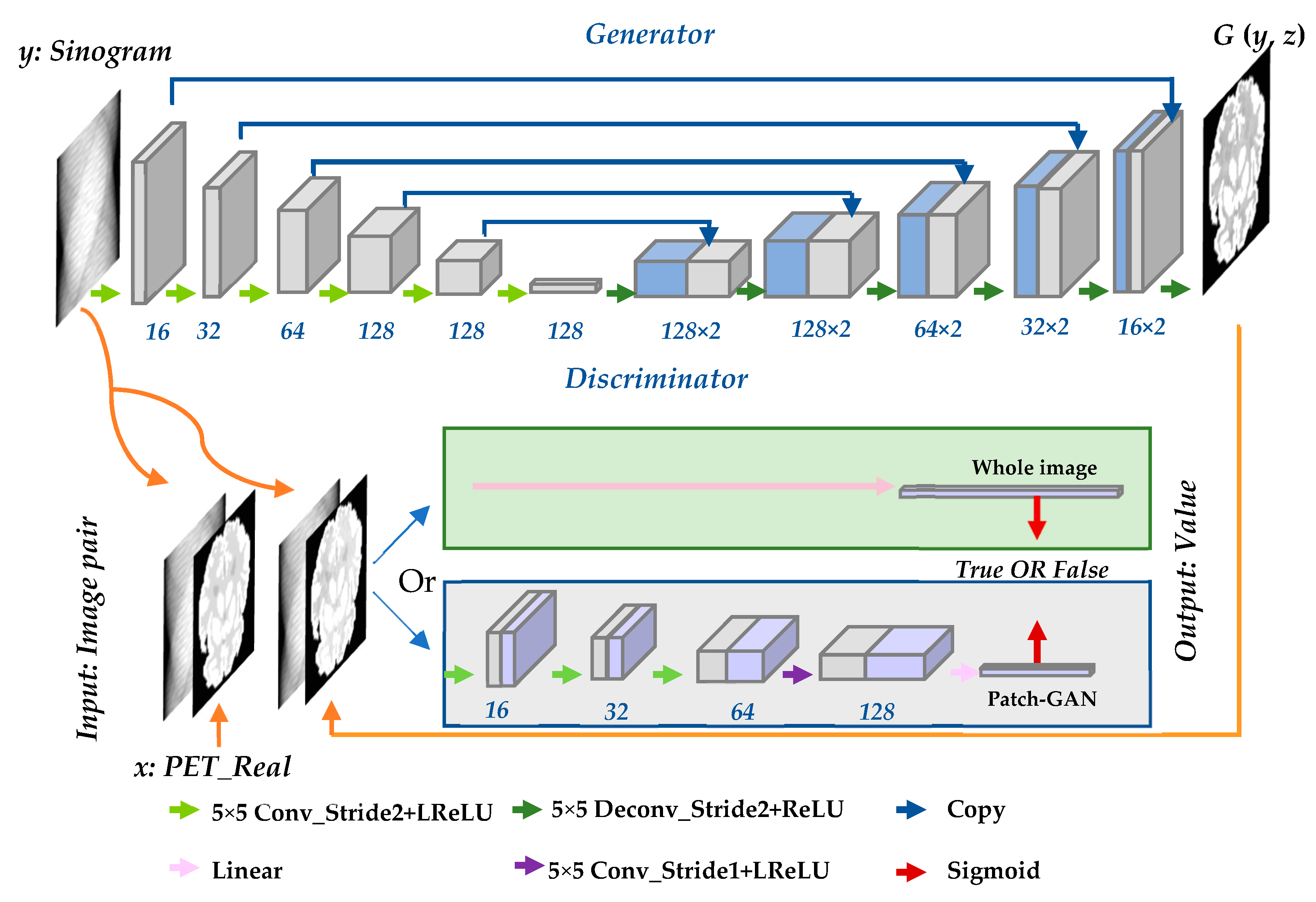
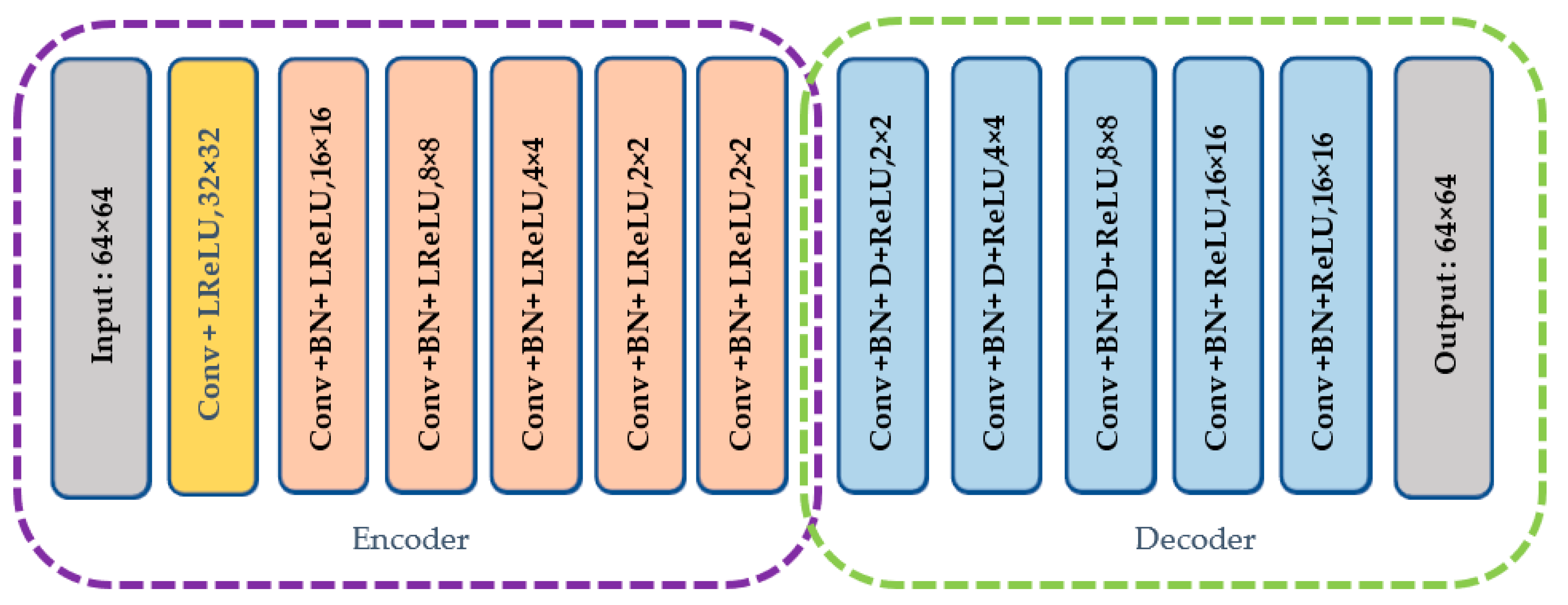
2.2.1. Network Design

Unlike traditional generative adversarial networks (GANs) [37], in which the only input is noise z, cGANs can provide extra information y to lead the training of the network. In this work, the input data include both noise z and sinogram data y. The cGANs consist of two models: generator G and discriminator D. The generator adapts the U-net architecture [38], which generates the PET image directly from a sinogram image. The full-image strategy is introduced to the discriminator, which attempts to differentiate between the real sinogram and PET image pairs from the database and the fake image pair output generated by G. The entire framework involves training G and D alternately until a balance is reached in the convergence stage. Figure 1 illustrates the structure of the entire reconstruction network. In the discriminator part, both the whole-image strategy and Patch-GAN strategy are utilized.

The generator consists of two paths. (1) Encoder: the contracting path (shown on the left-hand side of top of Figure 1 is used to compress the input image and obtain context information. (2) Decoder: the symmetrical expanding path (shown on the right-hand side) is used to expand the path and locate accurately. The basic module of both paths is convolution layer–batchnorm layer–ReLU layer. However, there are some differences in the details of the specific settings of encoding and decoding. There is no batch normalization (batchnorm) in the first layer of the encoder. All rectified linear units (ReLUs) in the encoder are leaky, whereas the ReLUs in the decoder are not leaky. All convolutions are 16 spatial filters and downsample with stride 2. Dropout is applied only to the first three layers of the decoder. Skip connections that concatenate activations from the layer in the contracting path to the (n − i)th layer are built in the expanding path, where n is the total number of layers. For the proposed method, n = 12. Finally, a tanh function is adopted after the last layer in the decoder to complete the entire generator model, and the output image has the same size as that of the input image. The structure of the generator is illustrated in Figure 2.

Patch-GAN is a very efficient strategy in image-to-image translation task. The Patch-GAN only penalizes structure at the scale of patches. This strategy tries to classify if each N × N patch in an image is real or fake. It can be understood as a form of texture/style loss. However, for reconstruction, the sinogram space is not correlated to image space as shown in Figure 3, which means the patch-based image to image translation may be not suitable for reconstruction task. The values of abscissa and ordinate of each pixel in the sinogram image have their own physical meaning. In actuality, each pixel in the sinogram related to the full activity image. Therefore, we attempt to perform it on the full space, which is called the whole-image strategy in this paper. The loss of the full image is adopted instead of the loss of each patch. The whole image and Patch-GAN discriminators were compared in this study. Both types of discriminators were tested in the simulation and SD rat experiments. Because the whole-image discriminator obtained a higher score in the compared experiments, all experiment results are based on the whole-image discriminator.

The Adam solver was used to optimize the networks. The number of training iterations n = 120, the learning rate α = 0.0002, and the weight of the L1 term λ = 100.

2.2.2. Objective Function

The conditional restriction can make the results closer to the desired ones. Therefore, the input includes both random noise z and condition y, and the objective of the cGAN can be represented as

$$L_{CGANs}\left(D,G\right)=E_{x,y~p_{data\left(x,y\right)}}\left[\log D\left(x,y\right)\right]+E_{x~p_{data\left(x\right)},z~p_{z\left(z\right)}}\left[\log (1-D\left(x,G\left(z,y\right)\right))\right]$$

(4)

As shown in Equation (4), generator G attempts to adjust parameters to minimize $\log (1-D\left(x,G\left(z,y\right)\right))$, while D tries to maximize it; thus, they are two adversarial models. Training according to adversarial loss makes the generated images clear but does not ensure similarity with the established image. To enhance the accuracy of low-frequency information, the L1 regularizer is introduced in the proposed model. Thus, the entire objective function can be described as

$$G^{*}=arg \underset{G}{\min } \underset{D}{\max }{L}_{CGANs}\left(D,G\right)+\mathsf{\lambda }{L}_{L1}\left(G\right)$$

(5)

where $L_{L1}\left(G\right)$ is the L1-norm, which is represented as

$$L_{L1}\left(G\right)=E_{x,y~p_{data}\left(x,y\right),z~p_z\left(z\right)}[\Vert x-G{\left(y,z\right)\Vert }_1].$$

(6)

3. Experiments

Simulation experiments, including the Zubal thorax phantom and Zubal brain phantom, SD rat experiments, and real patient experiments were designed to verify the performance of the algorithm.

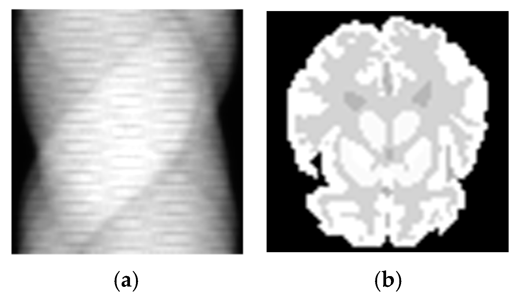
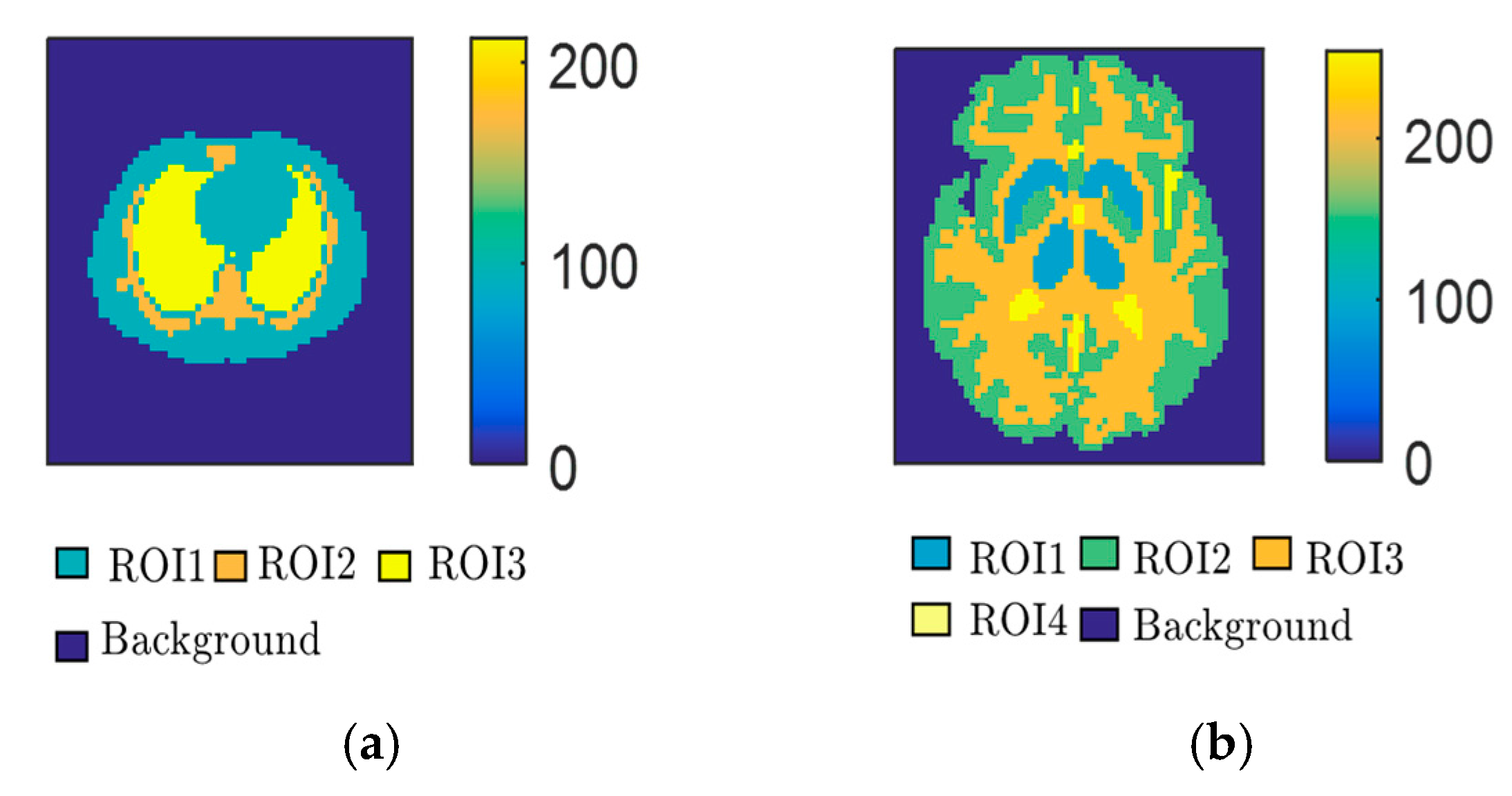
3.1. Simulation Experiments

Simulated data of the Zubal thorax phantom with ⁶⁴Cu-ATSM and Zubal brain phantom with 11C-Acetate were generated using Monte Carlo simulations, which can simulate the true environment of the PET scan and generate realistic sinogram data by using the GATE toolbox. The simulated PET scanner adopted was the Hamamatsu SHR74000, which contains six rings with 48 detector blocks. The ring diameter is 826 mm. The size of the field of view is 576 mm in the transaxial direction and 18 mm in the axial direction [39]. To obtain the original PET data for the Monte Carlo simulation, a two-compartment model was used to simulate the radiation concentration of different regions of interest (ROIs) in different phantoms. Figure 4 shows that each phantom is composed of several ROIs, in which the kinetic parameters of the two-compartment model are different. Details regarding the kinetic parameter settings can be found in the literature [40,41,42]. Each phantom consisted of three data sampling times. For each sampling time, three levels of counting rates were set: 5 × 10⁶, 1 × 10⁷, and 5 × 10⁷. For different counts, each reconstructed dynamic image had 18 frames with a resolution of 64 × 64 pixels. Thus, the entire database consisted of two phantoms, and each phantom dataset contained 162 (9 × 18) images. One third of each phantom dataset was randomly selected as the testing set, which included 162 images, with the others making up the training set, which included 324 images. The detailed sampling interval of the 18 frames is shown in

Table 1. Dataset for simulation experiments.

Phantom	Sampling Time	Sampling Interval	Counts	Dataset
Zubal thorax	20 min	14 × 50, 2 × 100, 2 × 150 s	5 × 106	training
			1 × 107
			5 × 107
	30 min	10 × 30, 2 × 150, 6 × 200 s	5 × 106	training
			1 × 107
			5 × 107
	40 min	10 × 30, 5 × 240, 3 × 300 s	5 × 106	testing
			1 × 107
			5 × 107
Zubal head	20 min	12 × 50 s	5 × 106	training
		2 × 50, 2 × 100, 2 × 150 s	1 × 107	testing
			5 × 107
	30 min	5 × 30, 7 × 100 s	5 × 106	training
		1 × 100, 3 × 150, 2 × 200 s	1 × 107	testing
			5 × 107
	40 min	5 × 30, 7 × 150 s	5 × 106	training
		6 × 200 s	1 × 107	testing
			5 × 107

. For example, for the 20 min simulated scanning of the Zubal thorax phantom, the first 14 frames were taken every 50 s, then two frames were taken every 100 s, and the last two frames were taken every 150 s.

In this study, the bias and variance were adopted for comparison.

$$bias=\frac{1}{n}{{\displaystyle \sum }}_{i=1}^n\frac{\left|{\widehat{x}}_i-x_i\right|}{x_i}$$

(7)

$$variance=\frac{1}{n-1} {{\displaystyle \sum }}_{i=1}^n{(\frac{{\widehat{x}}_i-{\overline{x}}_i}{x_i})}^2$$

(8)

where n denotes the overall number of pixels in the ROI, $\widehat{x_i}$ denotes the reconstructed value at voxel i, $x_i$ denotes the true value at voxel i, and $\overline{x_i}$ is the mean value of $x_i$.

3.2. SD Rat Experiments

To verify the reliability of the algorithm, twelve nine-week-old SD rats injected with 18F-FDG were scanned using a Siemens Inveon micro-PET scanner. Sinograms of 128 pixels × 160 pixels × 130 slices and activity images of 128 pixels × 128 pixels × 130 slices were obtained. The reconstruction method used was the ordered subset expectation maximization 3D algorithm (OSEM 3D) packaged in Siemens scanning software. Three rats were randomly selected for testing, and the other nine rats were used for training. Thus, there were 1170 image pairs in the training dataset and 390 image pairs in the testing dataset. Here, the images reconstructed using OSEM 3D were treated as the ground truth.

For the SD rat dataset, the relative root mean squared error (rRMSE) was used to evaluate the image quality.

$$\mathrm{rRMSE}=\sqrt{\mathrm{MSE}}/\overline{x}$$

(9)

$$\mathrm{MSE}=\frac{1}{n}{{\displaystyle \sum }}_{i=1}^n{\left(\widehat{x_i}-x_i\right)}^2$$

(10)

where x is the ground truth, $\widehat{x}$ is the reconstructed image, $\overline{x}$ is the ground truth average pixel value, and n is the number of image pixels.

3.3. Real Patient Experiments

To test the feasibility of the proposed method on human datasets, the method was also evaluated using a human brain PET dataset from nine real patients. The tracer injected into the patient was 18F-FDG. For each patient, 93 slices of reconstructed images and corresponding sinogram images were obtained. The reconstruction method was OSEM. The sizes of the images were set to 320 × 320. The last two objects were selected as the testing dataset, and the other seven objects were used as the training dataset. In addition to using rRMSE, structure similarity (SSIM) was used to evaluate the quality of the results.

$$\mathrm{SSIM}\left(x,y\right)=\frac{\left(2u_{\widehat{x}}{u}_x+c_1\right)\left(2{\sigma }_{x\widehat{x}}+c_2\right)}{\left(u_{\widehat{x}}{}^2+u_x{}^2+c_1\right)\left({\sigma }_x{}^2+{\sigma }_y{}^2+c_2\right)}$$

(11)

where u_x is the mean value of x, $u_{\widehat{x}}$ is the mean value of $\widehat{x}$, ${\sigma }_x{}^2$ is the variance of x, ${\sigma }_{\widehat{x}}{}^2$ is the variance of $\widehat{x}$, and ${\sigma }_{x\widehat{x}}$ is the covariance of x and $\widehat{x}$.

Here, c₁ = (k₁L)², c₂ = (k₂L)², k₁ = 0.01, and k₂ = 0.03; both c₁ and c₂ are constants used to maintain stability. In addition, L is the dynamic range of the pixel values.

4. Results

4.1. Simulation Experiments

The Zubal thorax phantom was used to select a suitable discriminator and show the convergence of the algorithm. A Zubal head phantom was also used to verify the robustness and testing time of the proposed method.

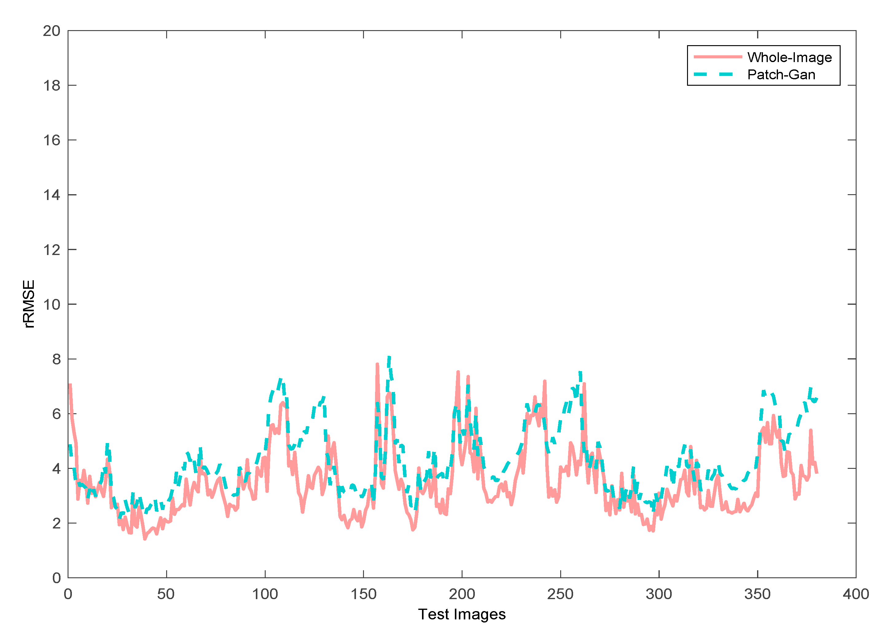
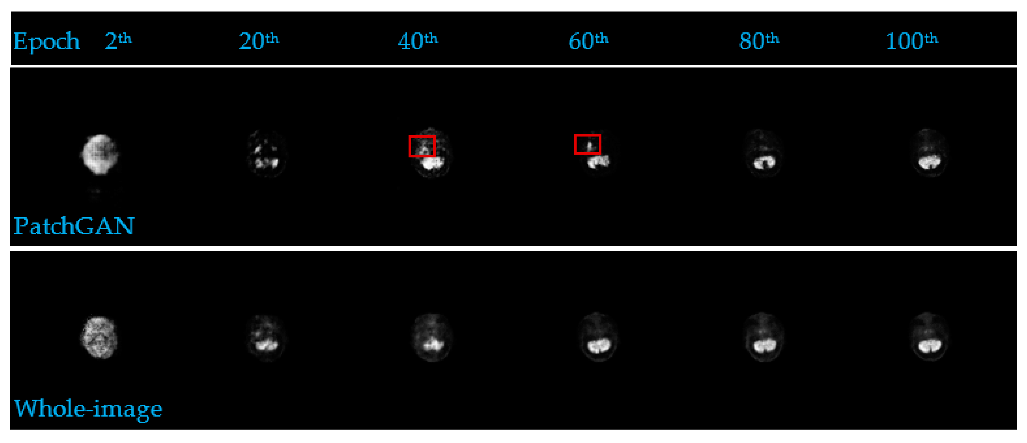
4.1.1. Discriminator Comparison Experiments

The full-image discriminator and Patch-GAN discriminator were both tested on the Zubal thorax dataset. Three dynamic objects were used to test, and each object possesses 18 frames. As we know, during the scanning period, with the increase in tracer injection time, the more photons the organ accumulates, the clearer the active image. In the current clinical practice, doctors usually pay attention to the static data, one clear active image of the later frames. Thus, the later frames are much useful for clinical. We compared the two strategies with the dynamic testing data and the results are shown in Figure 5. Though we obtained approximate quantitative results in the first 10 frames of the two strategies, the latter 8 frames of the whole-image strategy obtained much lower bias and variance compared to Patch-GAN. It is obvious that with the whole-image discriminator helping, the proposed network has better ability in improving the reconstruction image quality, especially for the frames with higher numbers of photons.

To better illustrate that the whole-image strategy is more suitable in PET reconstruction, we selected a real patient to show the generation results under different strategies at the same epoch in the training phase. The generation results of 2nd, 20th, 40th, 60th, 80th, and 100th epoch are all shown in Figure 6. With the increasing epoch, the global features become clearer for both strategies. However, the network with PatchGAN may generate some local features that do not exist in the ground truth, as shown in the red box. Moreover, compared with PatchGAN, a whole-image discriminator can generate more accurate reconstruction images in fewer epochs.

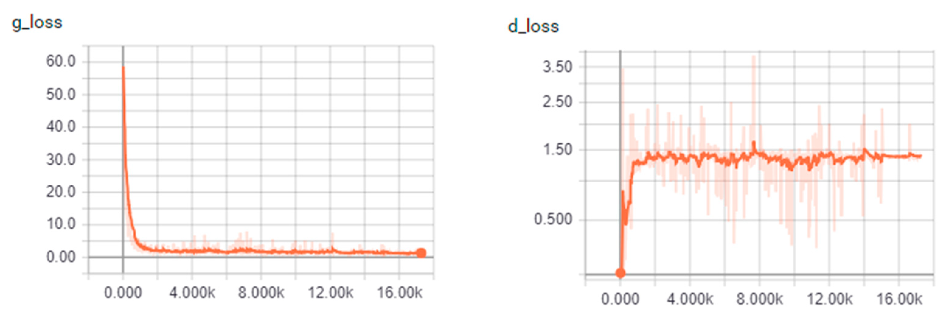
4.1.2. Convergence of the Algorithm

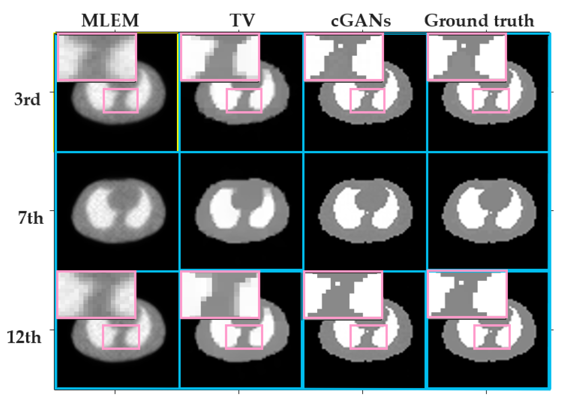
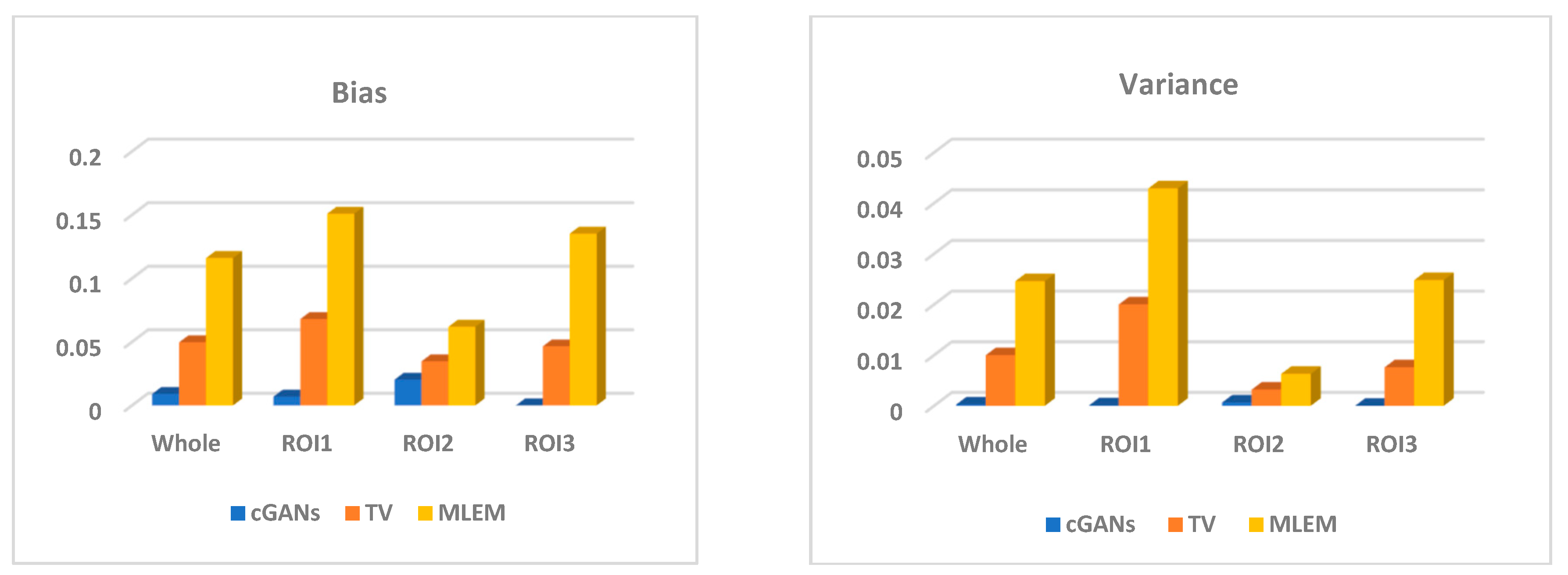
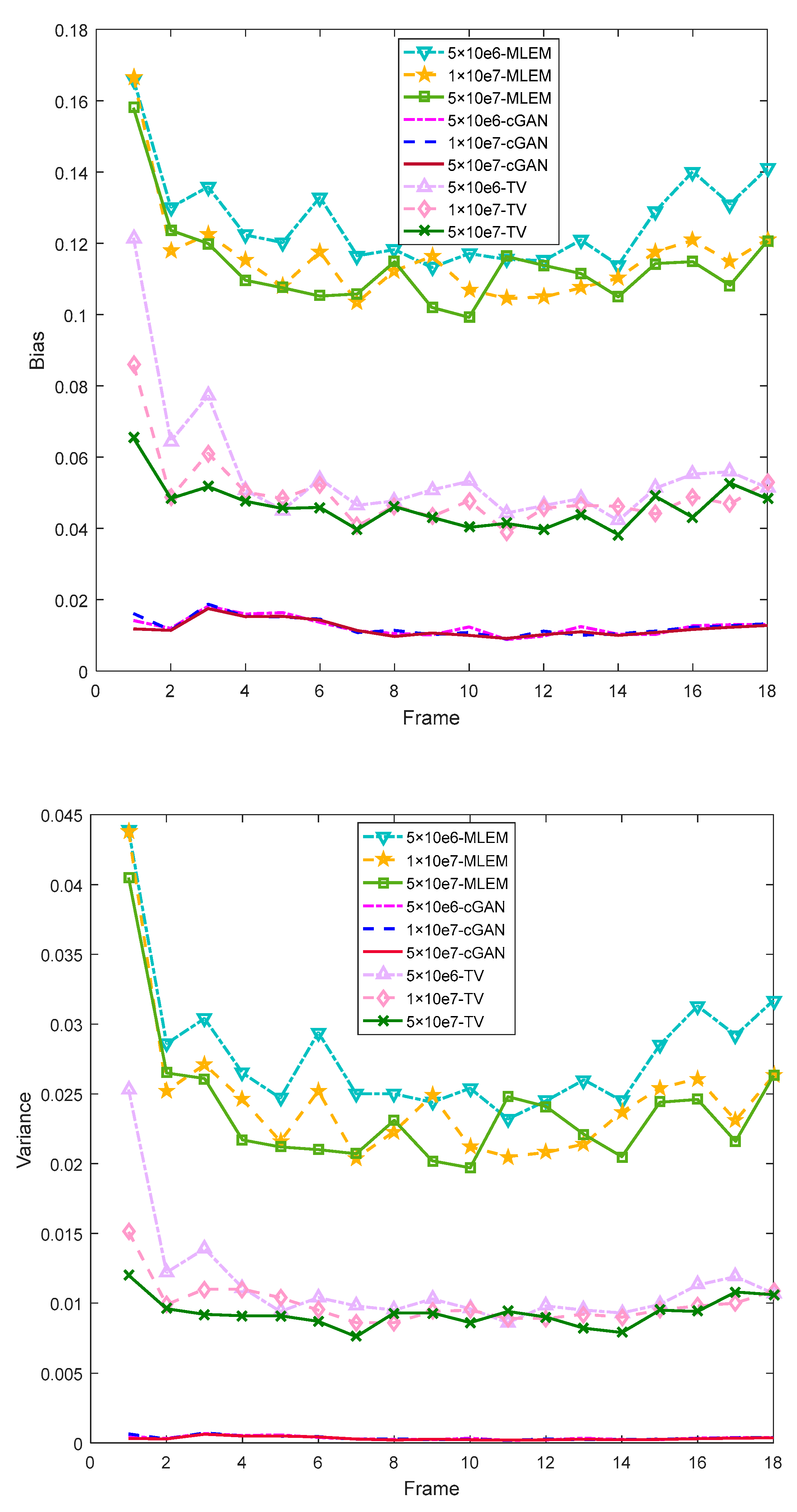
As shown in Table 1, the Zubal thorax dataset is divided according to sampling time. The 20 and 30 min scanning datasets belong to the training set, which contains 108 PET images and the corresponding sinogram images. The 40 min scanning data were chosen as the testing set, including 54 image pairs. The entire network was trained for 120 iterations, and the convergence curves are shown in Figure 7. The left curve shows the convergence of the discriminator, and the right curve represents the convergence of the generator. The x-axis indicates the loss value, and the y-axis indicates the iteration step. Both the generator and discriminator converge to a value quickly and tend to be stable.

4.1.3. Accuracy

Three frames of the Zubal thorax testing dataset were extracted to exhibit the reconstructed results, as shown in Figure 8. The method was also compared with the MLEM and TV algorithms. As shown in Figure 8, the reconstruction results of the proposed method are highly consistent with the ground truth in terms of the sharp edges and high pixel values of the ROIs. The results of the MLEM method contain excessive noise and artifacts because of the chessboard effect, even though the boundaries cannot be clearly observed. The TV method provides a clearer and sharper result than the MLEM method. However, the reconstruction effect of the small structure in the ROI3 area is poor, as indicated by the pink rectangular box. The detailed quantitative results are provided in

Table 2. Zubal thorax reconstruction evaluation results.

Frame	Method	Bias				Variance
		Total	ROI1	ROI2	ROI3	Total	ROI1	ROI2	ROI3
3rd	MLEM	0.1225	0.1739	0.0654	0.1284	0.0271	0.0510	0.0070	0.0233
	TV	0.0611	0.0909	0.0503	0.0420	0.0110	0.0227	0.0040	0.0063
	cGANs	0.0189	0.0112	0.0454	2.0 × 10−5	8.1 × 10−4	2.4 × 10−4	0.0022	7.8 × 10−8
7th	MLEM	0.1034	0.1335	0.0547	0.1221	0.0204	0.0356	0.0047	0.0210
	TV	0.0407	0.0586	0.0189	0.0446	0.0086	0.0168	0.0014	0.0077
	cGANs	0.0106	0.0066	0.0252	2.0 × 10−5	2.7 × 10−4	1.0 × 10−4	7.2 × 10−4	7.8 × 10−8
12th	MLEM	0.1049	0.1325	0.0573	0.1249	0.0208	0.0355	0.0055	0.0215
	TV	0.0457	0.0631	0.0342	0.0399	0.0089	0.0173	0.0025	0.0065
	cGANs	0.0042	0.0058	0.0068	1.0 × 10−5	6.7 × 10−5	8.9 × 10−5	1.1 × 10−4	3.9 × 10−8
18th	MLEM	0.1211	0.1545	0.0649	0.1439	0.0263	0.0444	0.0068	0.0277
	TV	0.0531	0.0689	0.0320	0.0584	0.0109	0.0195	0.0031	0.0103
	cGANs	0.0055	0.0067	0.0098	2.0 × 10−5	1.0 × 10−4	1.1 × 10−5	2.0 × 10−4	7.8 × 10−8

. The images generated by cGANs had less than one tenth of the bias and less than one percent of the variance of the full image compared to the MLEM. Compared to TV, we still found much lower bias and variance using cGANs. However, for different frames, the performance of cGANs has a great difference. For the first few frames, such as the third frame and seventh frame, though the cGANs obtained better quantitative results on full image compared with TV, the bias values of ROI2—which is a tiny area in the Zubal thorax phantom—are very close. For the late frames, such as the 12th and 18th frames, the bias values of cGANs are almost one tenth of TV’s. Even for the ROI2, cGANs also got surprised results. cGANs indeed has much stronger ability in the frames that own higher photons and less noise.

Figure 9 shows the mean values of the bias and variance of all 18 frames of the Zubal thorax phantom. For the bias and variance, the cGAN framework obtained a satisfactory score. The TV method performs much better performance than the MLEM method because it can better suppress the noise in the images. However, compared with the other two areas, the reconstruction results of ROI2 were unsatisfactory, and the values of the bias and variance of the three methods were higher than those of the other areas. It is considered that this outcome was possible because ROI2 was extremely small for it to be distinguished from the other two parts.

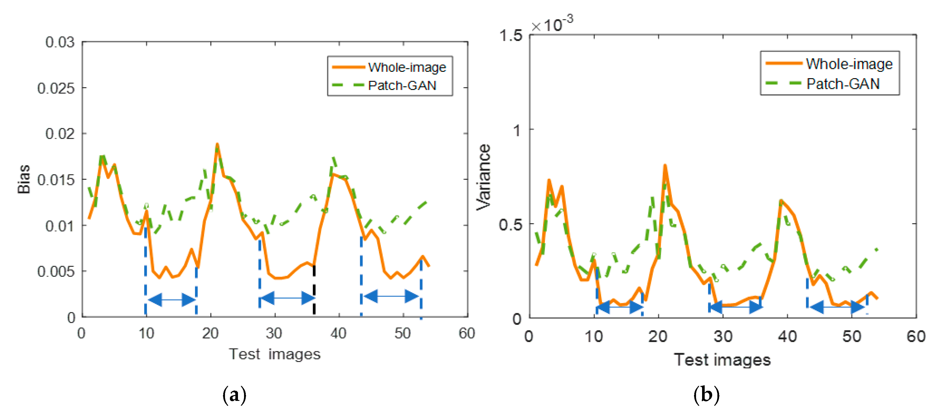
4.1.4. Robustness and Runtime Analysis

The Zubal thorax dataset was chosen to validate the robustness of the algorithm under different counting rates. The values of the evaluation parameters for reconstruction are shown in Figure 10. The three curves at the top of both the bias graph and the variance graph show the properties of MLEM, the three curves in the middle show the properties of TV, and the curves at the bottom show the properties of cGANs. The three solid curves at the bottom of the graph have the highest coincidence, which means that the cGAN method is the least affected by the count value. For the other two methods, as the count increases, both the variance and bias of the MLEM and TV methods decrease distinctly. Therefore, one can conclude that these two methods are significantly influenced by the count. This may be because both methods are based on a probabilistic statistical model; therefore, when the count increases, the probabilistic statistical characteristics of the data can be better guaranteed. Compared with the other two methods, the proposed framework has minimum variance and deviation and maximum stability.

The Zubal head phantom is more complex than the Zubal thorax phantom. It was used to verify whether the proposed algorithm can predict the reconstructed images of the last six frames by training the first 12 frames.

The concentration distribution of the first 12 frames is shown in Figure 11a. Four frames were chosen from the subsequent six frames to obtain the reconstruction results, as shown in Figure 11b. Although the training dataset did not include the last six frames, the test results are highly consistent with the true concentration distribution. Even an extremely small area, such as ROI3, can be reconstructed clearly, as indicated by the pink rectangular boxes in Figure 11b.

Table 3. Reconstruction times for Zubal thorax.

	Frame	2	4	6	8	10	12	14	16	18	Mean
Method
MLEM		0.213 s	0.211 s	0.204 s	0.215 s	0.218 s	0.210 s	0.207 s	0.217 s	0.202 s	0.211 s
TV		0.508 s	0.449 s	0.504 s	0.542 s	0.522 s	0.525 s	0.527 s	0.519 s	0.511 s	0.512 s
CGANs		0.007 s	0.007 s	0.007 s	0.007 s	0.007 s	0.007 s	0.007 s	0.007 s	0.007 s	0.007 s

and

Table 4. Reconstruction times for Zubal brain.

	Frame	13	14	15	16	17	18	Mean
Method
MLEM		0.219 s	0.268 s	0.226 s	0.233 s	0.260 s	0.260 s	0.244 s
TV		1.005 s	1.120 s	1.088 s	1.176 s	1.153 s	1.216 s	1.126 s
CGANs		0.007 s	0.007 s	0.007 s	0.007 s	0.007 s	0.007 s	0.007 s

listed the reconstruction results of three methods. As a classic traditional iterative method, MLEM cost about 0.2 s for reconstruction of each image. TV mixed a postprocessing of iterative method to improve the image quality, it takes almost twice as long as MLEM. As for cGANs, it only cost 0.007 s of each image because the model was trained in advance and the test time is very short which even can be ignored.

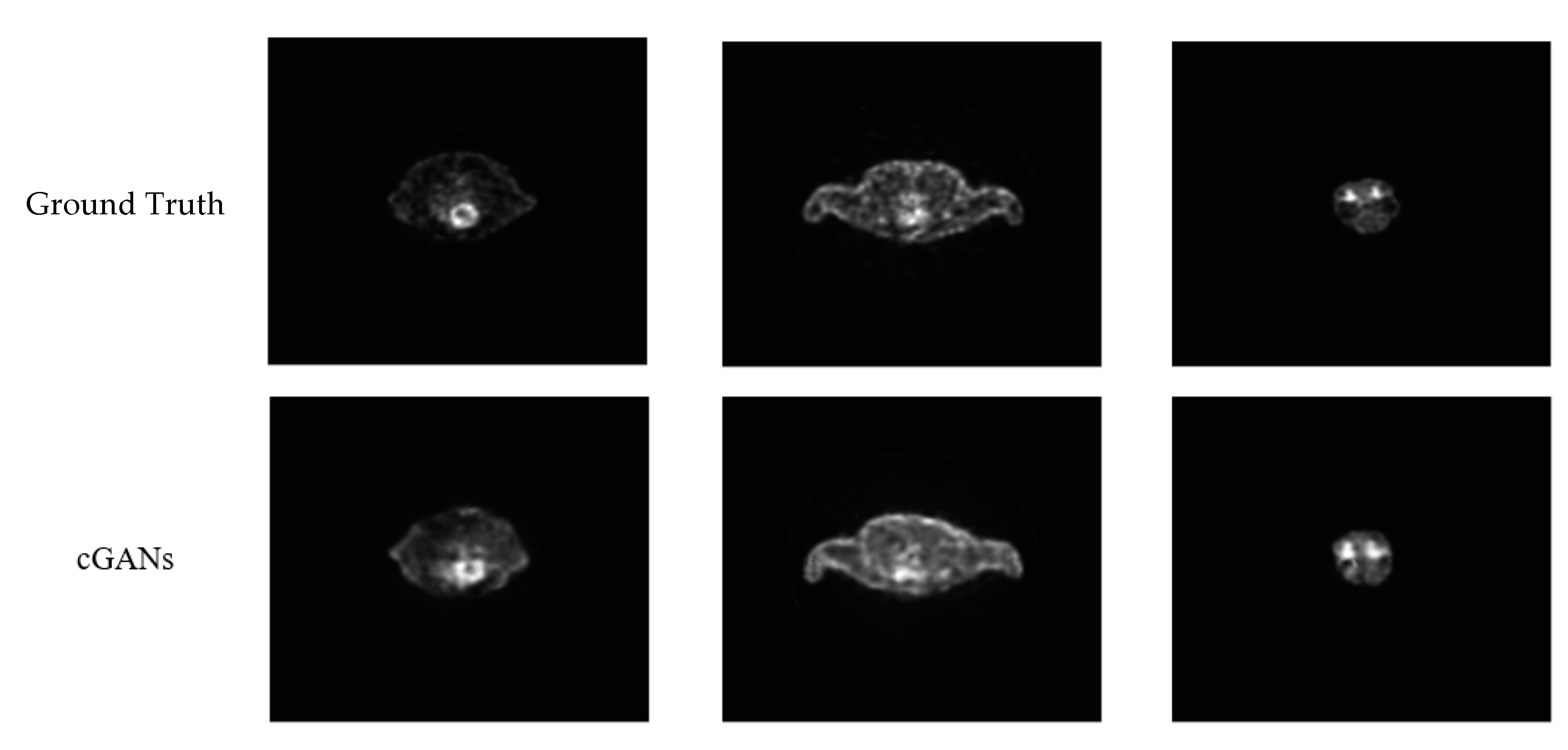
4.2. SD Rat Experiments

To verify the method in a faster and more familiar way, the sinogram and ground truth which generated with OSEM method were extended to a uniform size of 192 × 192 by zero padding. First, the two discriminators were compared on the real datasets. As shown in Figure 12, the rRMSE of the whole-image strategy is lower than that of Patch-GAN, which is consistent with the results of the simulations.

Three images in the test dataset were randomly chosen to obtain the reconstructed results. As shown in Figure 13, the reconstructed images produced by the cGAN have contour structures that are similar to the ground truth. However, the details are not clear, and the rRMSE value is slightly high. This may be caused by two factors: a more complex real scan situation and large individual differences among samples. A larger amount of data is required, but this is always a major challenge in medical image processing.

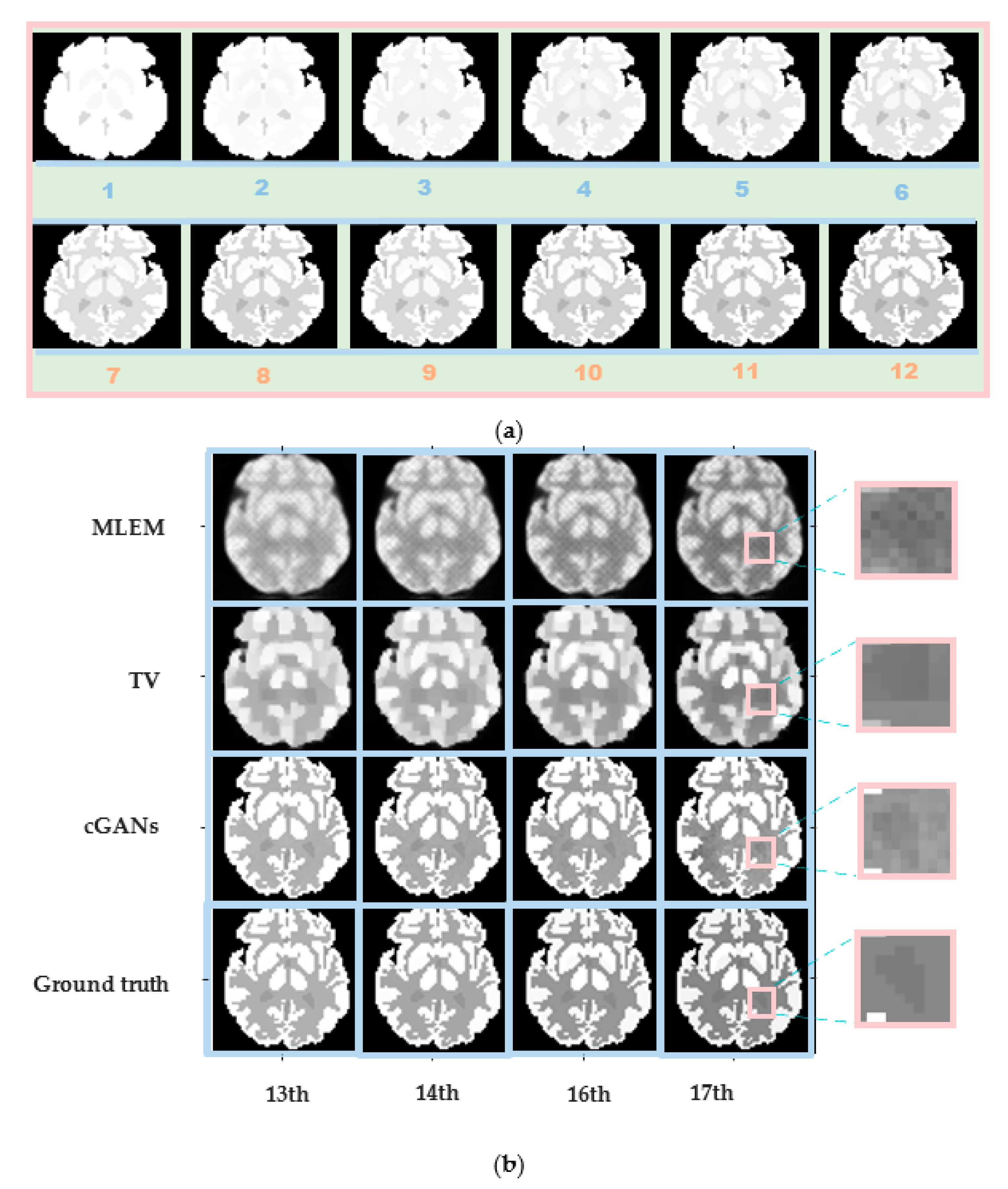
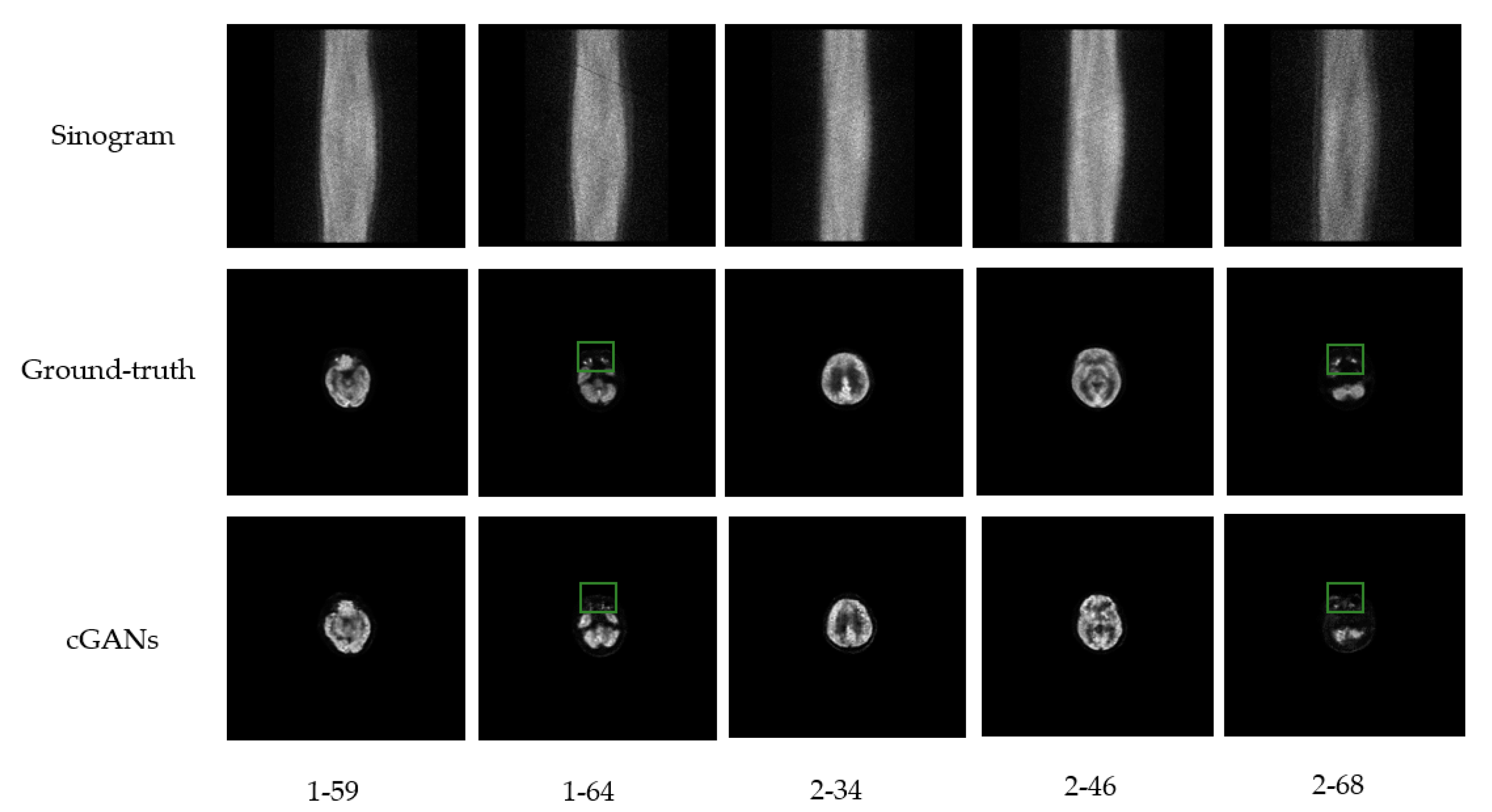
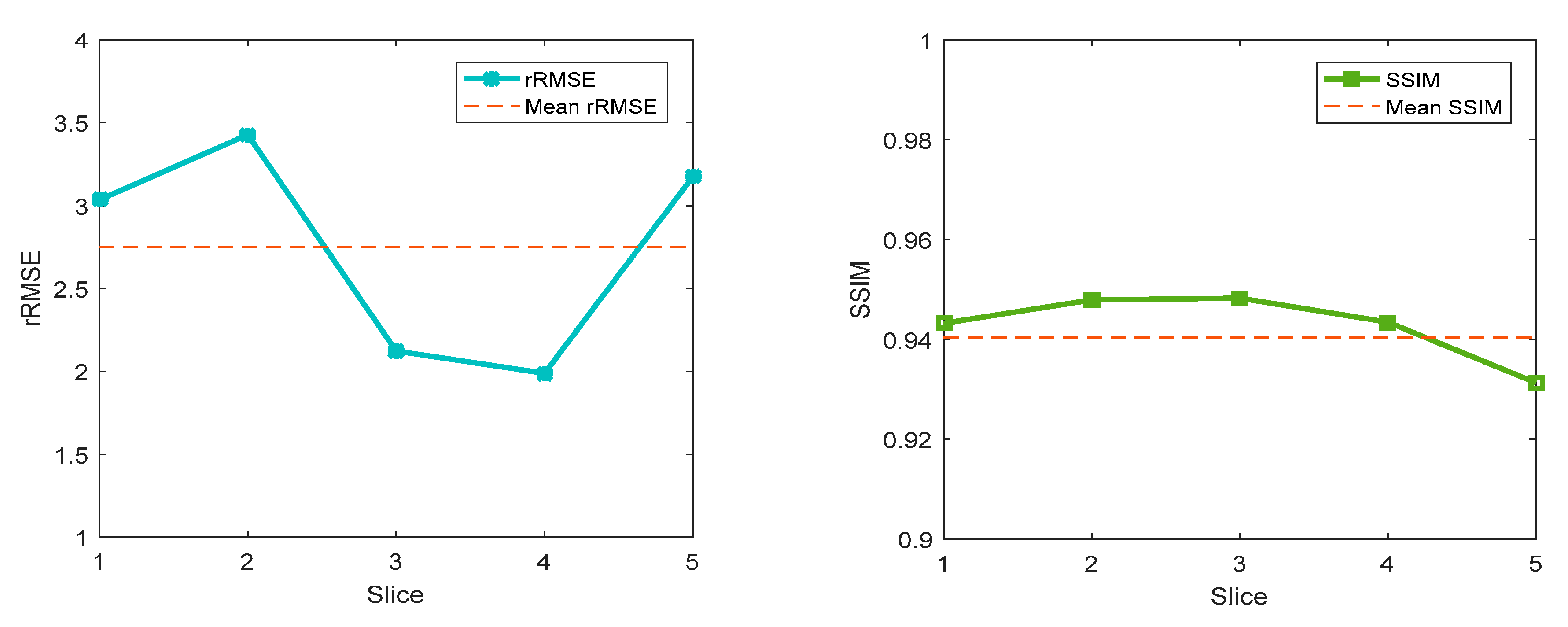
4.3. Real Patient Experiments

Several different learning rates and epochs were applied to a real human brain dataset. The best results were obtained with lr = 0.002 and 120 epochs. The training dataset contained seven objects, including 651 image pairs. The testing dataset contained two objects, which included 186 image pairs. Finally, five slices were selected from the test dataset, as shown in Figure 14. The quantitative results, including the SSIM and rRMSE, are shown in Figure 15. Compared to the SD rat whole-body dataset, the human brain dataset obtained better results in terms of reconstructed image quality. The SSIM of the test images was close to 0.94. The mean rRMSE was approximately 2.74. It is considered that the whole-body dataset of the SD rats may have finer and more complex structures than the human brain dataset. However, for a detailed structure, such as the green rectangle in Figure 14, it is difficult to obtain an accurate result. Unlike MLEM and TV, a single object can be reconstructed through a finite number of iterations; cGANs is a deep-learning-based method which achieve reconstruction by first learning the recognition processing of other objects. If there are not enough learning objects, then the leaning result is naturally not satisfied, and if the new object has some structures that the model has never seen before, it is very difficulty to reconstruct the new object accurately.

5. Discussion

PET has become an indispensable tool in clinical trials in recent years. The quality of the reconstructed image is crucial for the development of PET. However, traditional reconstruction methods have many limitations, as discussed above. Therefore, deep learning was adopted in this study to avoid the problems encountered in traditional methods. In this study, an attempt was made to learn the correspondence between sinogram images and reconstruction images. Considering that cGANs have obtained outstanding results in other fields, a cGAN was chosen as the main network. The results of the simulation, SD rat, and human brain datasets suggest that cGANs can outperform traditional methods.

For the simulation datasets, the reconstruction image quality is greatly improved compared with MLEM and TV, and the quantitative results also prove that. The bias values of cGANs for the first few frames are only 10% of that of MLEM method and about 30% of TV. The variance values are even less than 1% of the other methods. For the late frames which contain less noise and more photons, the bias and variance are much lower. For the reconstruction time, the deep-learning-based cGANs takes only 3% of the time of MLEM.

However, although satisfactory results were obtained for the simulation dataset, the performance on the SD rat and real patient datasets was not satisfactory. There are two reasons for this. First, the two real datasets had a more complex data acquisition environment. Moreover, there were significant differences between different individuals. Therefore, more data are required in the training data phase. Second, there was no additional information as a constraint in the network to guide the training process. Thus, it was difficult for the network to converge to more precise results.

In future work, more physiological information should be added to the network as an effective constraint. The inputs of the network can be multiple-scale images, which can lead the network to learn coarse and fine structures.

References

1. Kak, A.C.; Slaney, M.; Wang, G. Principles of Computerized Tomographic Imaging. Am. Assoc. Phys. Med. 2002, 29, 107. [Google Scholar] [CrossRef]
2. Shepp, L.A.; Vardi, Y. Maximum Likelihood Reconstruction for Emission Tomography. IEEE Trans. Med. Imaging 1982, 1, 113–122. [Google Scholar] [CrossRef] [PubMed]
3. Levitan, E.; Herman, G.T. A Maximum a Posteriori Probability Expectation Maximization Algorithm for Image Reconstruction in Emission Tomography. IEEE Trans. Med. Imaging 1987, 6, 185–192. [Google Scholar] [CrossRef] [PubMed]
4. Zhou, J.; Luo, L. Sequential weighted least squares algorithm for PET image reconstruction. Digit. Signal Process. 2006, 16, 735–745. [Google Scholar] [CrossRef]
5. Cabello, J.; Torres-Espallardo, I.; Gillam, J.E.; Rafecas, M. PET Reconstruction From Truncated Projections Using Total-Variation Regularization for Hadron Therapy Monitoring. IEEE Trans. Nucl. Sci. 2013, 60, 3364–3372. [Google Scholar] [CrossRef]
6. Verhaeghe, J.; D’Asseler, Y.; Vandenberghe, S.; Staelens, S.; Lemahieu, I. An investigation of temporal regularization techniques for dynamic PET reconstructions using temporal splines. Med. Phys. 2007, 34, 1766–1778. [Google Scholar] [CrossRef]
7. Marin, T.; Djebra, Y.; Han, P.K.; Chemli, Y.; Bloch, I.; El Fakhri, G.; Ouyang, J.; Petibon, Y.; Ma, C. Motion correction for PET data using subspace-based real-time MR imaging in simultaneous PET/MR. Phys. Med. Biol. 2020, 65, 235022. [Google Scholar] [CrossRef]
8. Higaki, T.; Nakamura, Y.; Tatsugami, F.; Nakaura, T.; Awai, K. Improvement of image quality at CT and MRI using deep learning. Jpn. J. Radiol. 2018, 37, 73–80. [Google Scholar] [CrossRef]
9. Wang, Y.; Yu, B.; Wang, L.; Zu, C.; Lalush, D.S.; Lin, W.; Wu, X.; Zhou, J.; Shen, D.; Zhou, L. 3D conditional generative adversarial networks for high-quality PET image estimation at low dose. NeuroImage 2018, 174, 550–562. [Google Scholar] [CrossRef]
10. Liu, H.; Xu, J.; Wu, Y.; Guo, Q.; Ibragimov, B.; Xing, L. Learning deconvolutional deep neural network for high resolution medical image reconstruction. Inform. Sci. 2018, 468, 142–154. [Google Scholar] [CrossRef]
11. Tezcan, K.C.; Baumgartner, C.F.; Luechinger, R.; Pruessmann, K.P.; Konukoglu, E. MR Image Reconstruction Using Deep Density Priors. IEEE Trans. Med. Imaging 2018, 38, 1633–1642. [Google Scholar] [CrossRef] [PubMed]
12. Luis, C.O.D.; Reader, A.J. Deep learning for suppression of resolution-recovery artefacts in MLEM PET image reconstruction. In Proceedings of the IEEE Nuclear Science Symposium and Medical Imaging Conference, NSS/MIC 2017, Atlanta, GA, USA, 21–28 October 2017. [Google Scholar]
13. Xie, S.; Zheng, X.; Chen, Y.; Xie, L.; Liu, J.; Zhang, Y.; Yan, J.; Zhu, H.; Hu, Y. Artifact Removal using Improved GoogleNet for Sparse-view CT Reconstruction. Sci. Rep. 2018, 8, 6700–6709. [Google Scholar] [CrossRef]
14. Kim, K.; Wu, D.; Gong, K.; Dutta, J.; Kim, J.H.; Son, Y.D.; Kim, H.K.; El Fakhri, G.; Li, Q. Penalized PET Reconstruction Using Deep Learning Prior and Local Linear Fitting. IEEE Trans. Med. Imaging 2018, 37, 1478–1487. [Google Scholar] [CrossRef]
15. Hong, X.; Zan, Y.; Weng, F.; Tao, W.; Peng, Q.; Huang, Q. Enhancing the Image Quality via Transferred Deep Residual Learning of Coarse PET Sinograms. IEEE Trans. Med. Imaging 2018, 37, 2322–2332. [Google Scholar] [CrossRef] [PubMed]
16. Han, Y.; Yoo, J.; Kim, H.H.; Shin, H.J.; Sung, K.; Ye, J.C. Deep learning with domain adaptation for accelerated projection-reconstruction MR. Magn. Reson. Med. 2018, 80, 1189–1205. [Google Scholar] [CrossRef] [PubMed]
17. Hammernik, K.; Klatzer, T.; Kobler, E.; Recht, M.P.; Sodickson, D.; Pock, T.; Knoll, F. Learning a variational network for reconstruction of accelerated MRI data. Magn. Reson. Med. 2017, 79, 3055–3071. [Google Scholar] [CrossRef] [PubMed]
18. Wang, S.; Su, Z.; Ying, L.; Peng, X.; Zhu, S.; Liang, F.; Feng, D.; Liang, D. Accelerating magnetic resonance imaging via deep learning. In Proceedings of the 2016 IEEE 13th International Symposium on Biomedical Imaging (ISBI), Prague, Czech Republic, 13–16 April 2016. [Google Scholar]
19. Kang, E.; Min, J.; Ye, J.C. A deep convolutional neural network using directional wavelets for low-dose X-ray CT reconstruction. Med. Phys. 2017, 44, e360–e375. [Google Scholar] [CrossRef]
20. Wu, D.; Kim, K.; Fakhri, G.E.; Li, Q. A Cascaded Convolutional Neural Network for X-ray Low-dose CT Image Denoising. arXiv 2017, arXiv:1705.04267. [Google Scholar]
21. Wang, T.; Lei, Y.; Fu, Y.; Wynne, J.F.; Curran, W.J.; Liu, T.; Yang, X. A review on medical imaging synthesis using deep learning and its clinical applications. J. Appl. Clin. Med. Phys. 2021, 22, 11–36. [Google Scholar] [CrossRef]
22. Cheng, Z.; Wen, J.; Huang, G.; Yan, J. Applications of artificial intelligence in nuclear medicine image generation. Quant. Imaging Med. Surg. 2021, 11, 2792–2822. [Google Scholar] [CrossRef]
23. Kawauchi, K.; Furuya, S.; Hirata, K.; Katoh, C.; Manabe, O.; Kobayashi, K.; Watanabe, S.; Shiga, T. A convolutional neural network-based system to classify patients using FDG PET/CT examinations. BMC Cancer 2020, 20, 227. [Google Scholar] [CrossRef] [PubMed]
24. Kumar, A.; Fulham, M.; Feng, D.; Kim, J. Co-Learning Feature Fusion Maps From PET-CT Images of Lung Cancer. IEEE Trans. Med. Imaging 2019, 39, 204–217. [Google Scholar] [CrossRef] [PubMed]
25. Protonotarios, N.E.; Katsamenis, I.; Sykiotis, S.; Dikaios, N.; Kastis, G.A.; Chatziioannou, S.N.; Metaxas, M.; Doulamis, N.; Doulamis, A. A few-shot U-Net deep learning model for lung cancer lesion segmentation via PET/CT imaging. Biomed. Phys. Eng. Express 2022, 8, 025019. [Google Scholar] [CrossRef] [PubMed]
26. Kumar, A.; Kim, J.; Wen, L.; Fulham, M.; Feng, D. A graph-based approach for the retrieval of multi-modality medical images. Med Image Anal. 2014, 18, 330–342. [Google Scholar] [CrossRef]
27. Gong, K.; Guan, J.; Kim, K.; Zhang, X.; Yang, J.; Seo, Y.; El Fakhri, G.; Qi, J.; Li, Q. Iterative PET Image Reconstruction Using Convolutional Neural Network Representation. IEEE Trans. Med. Imaging 2018, 38, 675–685. [Google Scholar] [CrossRef]
28. Gong, K.; Catana, C.; Qi, J.; Li, Q. Direct Reconstruction of Linear Parametric Images From Dynamic PET Using Nonlocal Deep Image Prior. IEEE Trans. Med. Imaging 2022, 41, 680–689. [Google Scholar] [CrossRef]
29. Huang, Y.; Zhu, H.; Duan, X.; Hong, X.; Sun, H.; Lv, W.; Lu, L.; Feng, Q. GapFill-recon net: A cascade network for simultaneously PET gap filling and image reconstruction. Comput. Methods Programs Biomed. 2021, 208, 106271. [Google Scholar] [CrossRef]
30. Lempitsky, V.; Vedaldi, A.; Ulyanov, D. Deep image prior. In Proceedings of the 2018 IEEE Conference on Computer Vision and Pattern Recognition, Salt Lake City, UT, USA, 18–13 June 2018. [Google Scholar]
31. Gong, K.; Catana, C.; Qi, J.; Li, Q. PET Image Reconstruction Using Deep Image Prior. IEEE Trans. Med. Imaging 2018, 38, 1655–1665. [Google Scholar] [CrossRef]
32. Song, T.-A.; Chowdhury, S.R.; Yang, F.; Dutta, J. Super-Resolution PET Imaging Using Convolutional Neural Networks. IEEE Trans. Comput. Imaging 2020, 6, 518–528. [Google Scholar] [CrossRef]
33. Häggström, I.; Schmidtlein, C.R.; Campanella, G.; Fuchs, T.J. DeepPET: A deep encoder–decoder network for directly solving the PET image reconstruction inverse problem. Med. Image Anal. 2019, 54, 253–262. [Google Scholar] [CrossRef]
34. Mirza, M.; Osindero, S. Conditional Generative Adversarial Nets. arXiv 2014, arXiv:1411.1784. [Google Scholar]
35. Isola, P.; Zhu, J.; Zhou, T.; Efros, A.A. Image-to-image translation with conditional adversarial networks. In Proceedings of the IEEE Conference on Computer Vision and Pattern Recognition, Honolulu, HI, USA, 21–26 July 2017; pp. 5967–5976. [Google Scholar]
36. Liu, Z.; Chen, H.; Liu, H. Deep Learning Based Framework for Direct Reconstruction of PET Images. In Proceedings of the Medical Image Computing and Computer Assisted Intervention—MICCAI 2019, 22nd International Conference, Shenzhen, China, 13–17 October 2019; pp. 48–56. [Google Scholar] [CrossRef]
37. Goodfellow, I.; Pouget-Abadie, J.; Mirza, M.; Xu, B.; Warde-Farley, D.; Ozair, S.; Bengio, Y.; Courville, A. Generative adversarial nets. Adv. Neural Inform. Processing Syst. 2014, 27, 1–9. [Google Scholar]
38. Ronneberger, O.; Fischer, P.; Brox, T. U-net: Convolutional networks for biomedical image segmentation. In Proceedings of the International Conference on Medical Image Computing and Computer-Assisted Intervention, Munich, Germany, 5–9 October 2015; Springer: Cham, Switzerland, 2015; pp. 234–241. [Google Scholar]
39. Fei, G.; Ryoko, Y.; Mitsuo, W.; Hua-Feng, L. An effective scatter correction method based on single scatter simulation for a 3D whole-body PET scanner. Chin. Phys. B 2009, 18, 3066–3072. [Google Scholar] [CrossRef]
40. Koeppe, R.A.; Frey, K.A.; Borght, T.M.V.; Karlamangla, A.; Jewett, D.M.; Lee, L.C.; Kilbourn, M.R.; Kuhl, D.E. Kinetic Evaluation of [11C]Dihydrotetrabenazine by Dynamic PET: Measurement of Vesicular Monoamine Transporter. J. Cereb. Blood Flow Metab. 1996, 16, 1288–1299. [Google Scholar] [CrossRef] [PubMed]
41. Muzi, M.; Spence, A.M.; O’Sullivan, F.; Mankoff, D.A.; Wells, J.M.; Grierson, J.R.; Link, J.M.; Krohn, K.A. Kinetic analysis of 3′-deoxy-3′-18F-fluorothymidine in patients with gliomas. J. Nucl. Med. 2006, 47, 1612. [Google Scholar] [PubMed]
42. Tong, S.; Shi, P. Tracer kinetics guided dynamic PET reconstruction. In Proceedings of the Biennial International Conference on Information Processing in Medical Imaging, Kerkrade, The Netherlands, 2–6 July 2007; Springer: Berlin/Heidelberg, Germany, 2007; p. 421. [Google Scholar]
Figure 1. Training framework of the direct reconstruction process.
Applsci 12 08118 g001
Figure 2. Architecture of generator.
Applsci 12 08118 g002
Figure 3. The sinogram image and the corresponding activate image. There is not a simple pixel-to-pixel relationship between (a,b). Each pixel of sinogram has its own physical meaning. The abscissa position of the pixel refers to the distance between line-of-response (LOR) and the center of the detector. The ordinate position of the pixel refers to the angle between LOR and the standard surface. The value of the pixel refers to the number of coincidence events recorded by the detector in the corresponding at this position.
Applsci 12 08118 g003
Figure 4. Two PET phantoms: (a) Zubal thorax phantom; (b) Zubal head phantom.
Applsci 12 08118 g004
Figure 5. Reconstruction results comparison of whole-image discriminator and Patch-GAN: (a) bias; (b) variance. The bias and variance of whole-image strategy are much lower than Patch-GAN of the later frames, as shown between the dashed blue line.
Applsci 12 08118 g005
Figure 6. The images generated in training phase under two different strategies. The first column shows the real brain images generated with PatchGAN. The second column shows the brain images generated with the whole-image method. From left to right: the images generated in the 2nd epoch, 20th epoch, 40th epoch, 60th epoch, 80th epoch, and 100th epoch.
Applsci 12 08118 g006
Figure 7. Convergence curves of the discriminator and generator. Both g-loss and d-loss converge quickly after approximately 1000 steps.
Applsci 12 08118 g007
Figure 8. Reconstruction results for Zubal thorax phantom with 40 min scanning and 1 × 10⁷ counts. From left to right: MLEM results, TV results, cGAN results, and ground truth. From top to bottom: the 3rd, 7th, and 12th frames.
Applsci 12 08118 g008
Figure 9. Bias and variance of whole images for ROI1, ROI2, and ROI3 of the Zubal thorax phantom.
Applsci 12 08118 g009
Figure 10. Bias and variance of three methods (MLEM, TV, and cGANs) of Zubal thorax phantom with different counts. The top three curves represent the results of the MLEM method, the middle curves represent results of the TV method, and the bottom curves correspond to the proposed method. With increasing counts, the bias and variance values of the MLEM and TV methods decrease, but there is a slight effect on the cGANs method.
Applsci 12 08118 g010
Figure 11. Robustness verification graphs of Zubal head phantom for different frames. (a) Concentration distribution of training images (the first 12 frames). (b) Reconstruction results for Zubal head phantom with a 70 min scan and 5 × 10⁷ counts. From top to bottom: MLEM results, TV results, cGAN results, and ground truth. From left to right: the 13th, 14th, 16th, and 17th frames.
Applsci 12 08118 g011
Figure 12. Comparison of reconstruction results using whole-image discriminator and patch-GAN on SD rat dataset.
Applsci 12 08118 g012
Figure 13. Reconstruction results of different slices of SD rats. From top to bottom: sinogram images, ground truth (OSEM), reconstruction results of cGANs.
Applsci 12 08118 g013aApplsci 12 08118 g013b
Figure 14. Reconstruction results of five selected images of human brain dataset: 1–59 depicts the 59th slice of the first test object, 2–34 depicts the 34th slice of the second test object, etc.
Applsci 12 08118 g014
Figure 15. Reconstruction results of five selected images of human brain dataset.
Applsci 12 08118 g015